10. Stellar Pulsation

10.1. Observations of Pulsating Stars

A Luthern pastor and amatuer astronomer David Fabricius was observing \(\omicron\) Ceti (omicron Ceti) in August 1595. The brightness of the star slowly faded over a period of \({\sim}\)2 months and vanished from the sky by October. The star eventually recovered and returned to its former brilliance after a couple of months. By 1662, the star was named Mira, which is Latin for astonishing. Also by this time, the 11-month period of its cycle was established.

Note

The regular changes in brightness were mistakenly attributed to dark “blotches” on the stellar surface. Supposedly, Mira would appear fainter when the dark areas were turned toward Earth.

Today astronomers recognize that the changes in Mira’s brightness are not due to dark spots on its surface, but to the fact that Mira is a pulsating star, or a star tha dims and brightens as its surface expands and contracts. Mira is the protoype of the long-period variables, or stars that have irregular light curves and pulsation periods between \(100-700\) days.

Fig. 10.1 Light curve of Mira. Image credit: Wikipedia:Mira.

The next pulsating star was discovered in 1784 by John Goodricke of York, England. He found that the brightness of \(\delta\) Cephei varies regularly with a period of 5.367 days (or 5 days, 8 hours, 48 minutes). Goodricke contracted pneumonia while observing \(\delta\) Cephei and died at the age of 21. \(\delta\) Cephei is different than Mira, in that it varies by less than one magnitude in brightness and never fades from view. Pulstation stars similar to \(\delta\) Cephei are called classical Cepheids and are vitally important to astronomy.

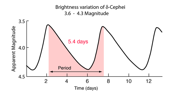
Fig. 10.2 Light curve of \(\delta\) Cephei. Image credit: Hyperphysics:delta Cephei.

10.1.1. The Period-Luminosity Relation

In the early 20th century, Henrietta Swan Leavitt was hired at Harvard University to compare photographic plates of the same field of stars taken at different times and detect any star that varied in brightness. Eventually she discovered 2400 classical Cepheids with perios between \(1-50\) days, where most of them were located in the Small Magellanic Cloud (SMC). Leavitt noticed that the more lumious Cepheids took longer to complete their pulsation cycles, where she compared the apparent magnitudes of the these SMC stars against their pulsation periods. As a result, she demonstrated that the apparent magnitudes of classical Cepheids are closely correlated with their peirods, with an uncertainty of only \(\Delta m \approx \pm 0.5\) at a given period.

Fig. 10.3 Comparision of the apparent magnitude of the SMC stars (y-axis) with respect to their pulsation periods (in days). Image credit: Wikipedia:Henrietta Swan Leavitt.

The distance to the SMC is large compared to the distance between stars, so we can assume that all the stars in SMC are roughly the same distance from us (about 91 kpc). The differences in their apparent magnitudes must be the same as the differences in their absolute magnitudes. The observed differences in the apparent brightness of the stars must reflect intrinsic differences in their luminosities.

Accurate distances to stars (via parallax) are limited to only the nearest (less than \({\sim}\)10 kpc with the Gaia spacecraft) from us due to the ambiguity in a star’s apparent brightness as a function of distance. Astronomers were excited at the prospect of determing the absolute magnitude (or luminosity) of a distant Cepheid simply by timing its pulsation. Recall that the difference between a star’s apparent and absolute magnitude allows for the an independent distance calculation via the distance modulus. This would permit the measurement of large distances in the universe.

The only stumbling block was the calibration of Leavitt’s relation. An independent distance to a single Cepheid had to be obtained to measure its absolute magnitude and luminosity. The resulting period-luminosity relation could be used to measure the distance to any Cepheid.

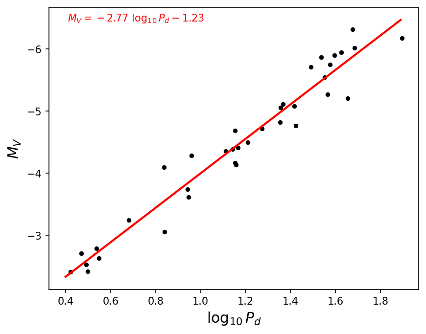
The nearest classical Cepheid is Polaris (some 200 pc away). In the early 20th century, this distance was much to great to be measured via stellar parallax. However, Hertzsprung (in 1913) succeed by using the longer baseline provided by the Sun’s motion through space (along with statistical methods) to find the distances to Cepheids haveing a specified period. The calibrated period-luminosity relation for the \(V\) band is described by

(10.1)\[M_{\langle V \rangle} = -2.81 \log_{10}{P_d} - 1.43,\]

where \(M_{\langle V \rangle}\) represents the average absolute \(V\) magnitude and \(P_d\) is the pulsation period in days. In terms of the average stellar luminosity, the relation is given by

(10.2)\[\begin{align} \log_{10}{\frac{\langle L \rangle}{L_\odot}} = 1.15 \log_{10}{P_d} + 2.47. \end{align}\]

The python code below shows a linear fit to visual magnitude \(M_V\) and pulsation periods \(P_d\) from Cepheids in the Large Magellanic Cloud, LMC, (Strom et al. (2011)). This fit reasonably matches the coefficients given in Eqn. (10.1).

import numpy as np
import matplotlib.pyplot as plt

#Using data from Strom et al. (2011)
#https://www.aanda.org/articles/aa/pdf/2011/10/aa17154-11.pdf

logP, M_V, M_J, M_H, M_K = np.genfromtxt("Strom_Table3.dat",usecols=(1,6,7,9,10),unpack=True)  #log P, M_V, M_J, M_K

#calculate Period-Luminosity Relation
z = np.polyfit(logP,M_V,1)
PL = np.poly1d(z)

width = 5
ms = 7
lw = 2
fs = 'x-large'

fig = plt.figure(figsize=(1.3*width,width),dpi=150)
ax = fig.add_subplot(111)

ax.plot(logP,M_V,'k.',ms=ms)
logP_rng = np.arange(0.4,1.9,0.01)
ax.plot(logP_rng,PL(logP_rng),'r-',lw=lw)
ax.invert_yaxis()


ax.text(0.05,0.95,"$M_V = %1.2f\ \log_{10}{P_d} - %1.2f$" % (z[0],np.abs(z[1])),color='r',horizontalalignment='left',transform = ax.transAxes)
ax.set_xlabel("$\log_{10}{P_d}$",fontsize=fs)
ax.set_ylabel("$M_V$",fontsize=fs);

A problem of measuring stars in the \(V\) band is interstellar extinction and reddening is more signficant. Astronomers can substantially decrease the scatter in the period-luminosity relation by making observations at infrared wavelengths, where interstellar extinction is less of a problem. A fit of the period-luminosity relation in the infrared \(H\) band is given by

(10.3)\[\begin{align} H = -3.234 \log_{10}{P_d} + 16.079. \end{align}\]

The scatter can be further reduced by adding a color term to the fit because a star’s color is independent of its distance. Using the infrared color index \(J-K\), the fit becomes much tighter. Note that the \(J\) band is centered on \(1.215\ {\rm \mu m}\), where the \(K\) band is centered on \(2.157\ {\rm \mu m}\). Using the color index, the period-luminosity-color relation is given by

(10.4)\[\begin{align} H = -3.428 \log_{10}{P_d} + 1.54 \langle J-K \rangle + 15.637. \end{align}\]

Classical Cepheids provide astronomy with its third dimension and supply the foundation for the measurement of extragalactic distances. Cepheids are super giant stars (hence the pulsation), which are about \(50\ R_\odot\) and 1000s of times more luminous, means that they can be seen over intergalactic distances. They serve as “standard candles,” or beacons scattered through the night sky that serve as guideposts for astronomical surveys of the universe.

10.1.2. The Pulsation Hypothesis for Brightness Variations

A detailed understanding of the physical reasons for the light variations of Cepheids is no required to appreciate the important ues of Cepheids as cosmic distance indicators. The observed changes in brightness were once thought to have originated with the tidal effects of binary stars.

In 1914, Harlow Shapley argued that the binary theory was fatally flawed because the stellar size needed would exceed the binary orbit. Shapley advanced an alternative idea:

The observed variations in the brightness and temperature of the classical Cepheids were caused by radial pulsations of single stars. He proposed that these stars were rhythmically “breathing” in and out, which corresponded to the process of brightening and dimming.

Four years later Eddington provided a firm theoretical framework for the pulsation hypothesis, which received strong support from the observed correlations among the variations in brightness, temperature, and surface velocity throughout the pulsation cycle.

The change in brightness is primarily due to the \({\sim}1000\ {\rm K}\) variation in the surface temperature of \(\delta\) Cephei. The accompaning change in size makes a lesser contribution to the luminosity. Although the total excursion of \(\delta\) Cephei’s surface from its equilibrium radius is large in absolute terms (\(\gtrsim 1R_\odot\)), it is still only \({\sim}5-10\%\) the size of a supergiant star.

The spectral type of \(\delta\) Cephei changes continuously through the cycle from \({\rm F5-G2}\) (hottest-coolest). A careful examination of Fig. 10.4 shows that the magnitude and surface velocity curves are nearly identical in shape. The star is brightest when its surface is expanding outward most rapidly, after it has passed through its minimum radius. The phase lag of maximum luminosity is due to the mechanism that maintains its oscillations.

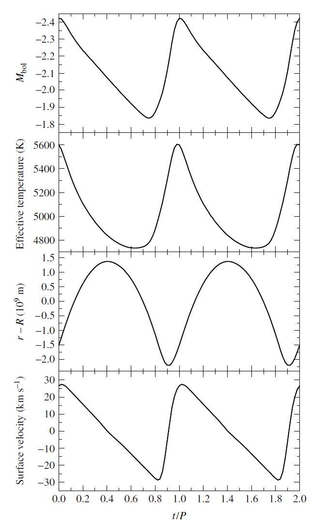
Fig. 10.4 Observed pulsation properties of \(\delta\) Cephei. Image credit: Carroll & Ostlie (2007); Data from Schwarzchild (1938).

10.1.3. The Instability Strip

The Milky Way is estimated to contain several million pulstating stars. Given that the total number of stars is several hundred billion, this means that stellar pulsation must be a transient phenomenon. The positions of the pulsating variables on the H-R diagram confirm this conclusion.

Fig. 10.5 Variable stars on an H-R diagram schematic. Image credit: Christensen-Dalsgaard (2004).

Rather than being located on the main sequence, the majority of pulsating stars occupy a narrow (\({\sim}600-1100\ {\rm K}\) wide), nearly vertical instability strip on the right-hand side of the H-R diagram. Stars evolve along tracks towards the RGB and begin to pulsate as the enter the instability strip and cease their oscillations upon leaving.

10.1.4. Some Classes of Pulsating Stars

Astronomers have divided pulsating stars into several classes. Some of these are listed below.

Table 10.1 Pulsating Stars

Type	Period Range	Population Type	Radial or Nonradial
Long-Period Variables (LPV)	\(100-700\ {\rm days}\)	I, II	R
Classical Cepheids	\(1-50\ {\rm days}\)	I	R
W Virginis stars	\(2-45\ {\rm days}\)	II	R
RR Lyrae stars	\(1.5-24\ {\rm hours}\)	II	R
\(\delta\) Scuti stars	\(1-3\ {\rm hours}\)	I	R, NR
\(\beta\) Cephei stars	\(3-7\ {\rm hours}\)	I	R, NR
ZZ Ceti	\(100-1000\ {\rm seconds}\)	I	NR

The W Virginis stars are metal-deficient (Pop. II) Cepheids and are about \(4\times\) less luminoius than classical Cepheids with the same period. Their period luminosity relation is thus lower than and parallel to the one shown for the classical Cepheids.

RR Lyrae stars (Pop. II) are horizontal-branch stars found in globular clusters. Since all RR Lyrae stars have nearly the same luminosity, they are also useful as standard candles for distance measurements.

The \(\delta\) Scuti variables are evovled \(\rm F\) stars found near the main sequence. They exhibit both radial and nonradial oscillations, where the latter is a more complicated motion than will be discussed later. Below the main sequence are the pulsating white dwarfs called ZZ Ceti stars.

The above listed star types (W Vir, RR Lyr, \(\delta\) Scu, and ZZ Cet) lie far within the instability strip, and they share a common mechanism that drives the oscillations. The long-period variables (e.g., Mira and \(\beta\) Cephei stars) are located outside of the instability strip occupied by the classical Cepheids and RR Lyrae stars.

10.2. The Physics of Stellar Pulsation

A wealth of knowledge has been obtained about the Earth’s interior using seismic waves produced by earthquakes and other sources. In the same manner, astrophysicists model the pulsational properties of stars to better understand their internal structure. By numerically evaluating an evolutionary sequence of stellar models and comparing the pulsational characteristics (e.g., periods, amplitudes, etc.) of the models with observations, astronomers can further test their theories of stellar structure and evolution. Moreover, they obtain a detailed view of the stellar interior in the process.

10.2.1. The Period-Density Relation

The radial oscillations of a pulsating star are the result of sound waves resonating in the stellar interior. A rough estimate of the pulsation period \(\Pi\) can be obtained by considering how long it would take a sound wave to traverse across a model star of radius \(R\) and constant density \(\rho\). Recall that the adiabatic sound speed is given by

\[\begin{align*} v_s = \sqrt{\frac{\gamma P}{\rho}}, \end{align*}\]

where \(P\) represents the pressure.

Note

The pulsation period is represented using \(\Pi\) so that it is not confused with the pressure \(P\). While another symbol \(T\) could be used for period, it could lead to confusion with temperature. Therefore \(\Pi\) is commonly used for pulsation period in stellar pulsation theory studies.

The pressure can be found for hydrostatic equilibrium, using the (unrealistic) assumption of constant density, which gives

(10.5)\[\frac{dP}{dr} = -\frac{GM_r\rho}{r^2} = -\frac{4\pi}{3}G\rho^2 r.\]

Using the boundary condition \(P=0\) at the surface, Eqn. (10.5) can be integrated to get the pressure as a function of \(r\),

(10.6)\[\begin{align} P(r) = \frac{2\pi}{3} G\rho^2 (R^2-r^2). \end{align}\]

The pulsation period is roughly

(10.7)\[\begin{split}\Pi &\approx 2 \int_{0}^R \frac{dr}{v_s} \approx 2 \int_{0}^R \frac{dr}{\sqrt{\frac{2\pi}{3}G\rho (R^2 -r^2)}}, \\ & \approx \frac{2}{\sqrt{\frac{2\pi}{3}G\rho }}\int_{0}^R \frac{dr}{\sqrt{R^2 - r^2}}, \\ & \approx \sqrt{\frac{3\pi}{2\gamma G \rho}}.\end{split}\]

This shows that a star’s pulsation period is inversely proportional to the square root of its mean density. This period-mean density relation explains why the pulsation period decreases as we move down the instability strip from the (low density) supergiants to the very dense white dwarfs (See Fig. 10.5).

Note

Pulsating white dwarfs exhibit nonradial oscillations, and their periods are longer than predicted by the period-mean density relation.

The tight period-luminoisty relation discovered by Leavitt exists because the instability strip is roughly parallel to the lumionisty axis of the H-R diagram in Fig. 10.5. The quantitative agreement between Eqn. (10.7) with the observed periods of Cepheids is not too bad, considering the assumptions.

Consider a typical Cepheid having a mass and radius of \(5\ M_\odot\) and \(50\ R_\odot\), respectively. Then \(\Pi \approx 10\ {\rm days}\). This falls within the range of periods measured for the classical Cepheids.

10.2.2. Radial Modes of Pulsation

The sound waves involved in radial modes of stellar pulsation are essentially standing waves, similar to the standing waves that occur in an organ pipe that is open at one end. Both the star and the organ pipe can sustain several oscillation modes. The standing wave for each mode has

• a node at one end (the star’s center; the pipe’s closed end), where the gases do not move, and

• an antinode at the other end (the star’s surface; the pipe’s open end).

For the fundamental mode, the gases move in the same direction at every point in the star or pipe. There is a single node between the center and the surface, which represents the first overtone mode, with the gases moving in opposite directions on either side of the node, and two ndes for the second overtone.

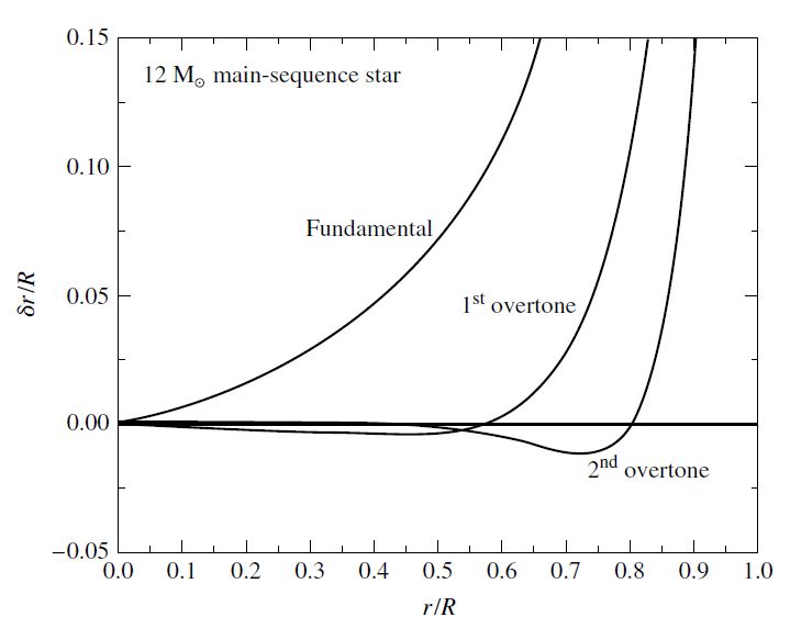
Fig. 10.6 Radial modes for a pulsating star. The waveform for each mode has been arbitrarily scaled so that \(\delta r/R = 1\) at the stellar surface. The maximum surface ratio \(\delta r/R = 0.05-0.10\) for a classical Cepheid. Figure credit: Carroll & Ostlie (2007).

For radial modes, the motion of the stellar material occurs primarily in the surface regions while some oscillation occurs deep inside the star. This effect is most prominent for the fundamental mode, where non-negligible amplitudes exist.

The vast majority of the classical Cepheids and W Virginis stars pulsate in the fundamental mode. The RR Lyrae variables pulsate in either the fundamental or the first overtone, with a few oscillations in both modes simultaneously. The long-period variables (LPVs) may also oscillate in either the fundamental mode or the first overtone.

10.2.3. Eddington’s Thermodynamic Heat Engine

To explain the mechanism that powers these standing sound waves, Eddington proposed that pulsating stars are thermodynamic heat engines. The gases comprising the layers of the star do thermodynamic work \((PdV)\) as they expand and contract throughout the pulsation cycle.

• If \(\oint P dV > 0\) for the cycle, a layer does net positive work on its surroundings and contributes to driving the oscillations;

• If \(\oint P dV < 0\), the net work is negative and tends to dampen the oscillations.

• If the total work (found by adding up the contributions from all the layers) is positive, the oscillations will grow in amplitude.

• If the total work is negative, then the oscillations will decay.

These changes in pulsation amplitude continue until an equilibrium value is reached, when the total work done by all the layers is zero.

As for any heat engine, the net work done by each layer of the star during one cycle is the difference between heat flowing into the gas and the heat leaving the gas. For driving, the heat must enter the layer during the high-temperature part of the cycle and leave during the low-temperature part.

Note

Just as the spark plug in an internal combustion engine (ICE) fires at the end of the compression stroke, the driving layers of a pulsating star must absorb heat around the time of their maximum compression. In this case, the maximum pressue will occur after maximum compression, and the oscillations will be amplified.

10.2.4. The Nuclear \(\epsilon\) Mechanism

Where within the star could the driving take place? Eddington considered that when the center of the star is compressed, its temperature and density rise which increase the thermonuclear energy generation rate \(\epsilon\).

However, there is a node at the center of the star. The pulsation amplituded is very small near the center. Although this energy mechanism (\(\epsilon\) mechanism) operates in the core of a star, it is usually not enough to drive the star’s pulsation. Variations in the thermonuclear energy generation rate \(\epsilon\) produce oscillations that may prevent the formation of \(\gtrsim 90\ M_\odot\) stars.

10.2.5. Eddington’s Valve

With the failure of the \(\epsilon\) mechanism, Eddington suggested an alternative, a valve mechanism.

Consider if a layer of the star became more opaque upon compression, then it could “dam up” the energy flowing toward the surface and push the surface layers upward. As this expanding layer became more transparent, the trapped heat could escape and the layer would fall back down to begin the cycle anew.

To apply this method, we must make the star more heat-tight when compressed than when expanded. –Sir Arthur Stanley Eddington

In other words, the opacity must increase with compression.

In most regions of the star, the opacity actually decreases with compression. For a Kramers law, the opacity \(\kappa\) depends on the density and temeperature of the stellar material as \(\kappa \propto \rho T^{-3.5}\). As the layers of a star are compressed, their density and temperature both increase. The opacity is more sensitive to the temperature than to the density, and the opacity usually decreases upon compression.

It takes special circumstances to overcome the damping effect of most stellar layers, which explains why stellar pulsation is so rare (only 1 out of every \(10^5\) stars).

10.2.6. Opacity Effects and the \(\kappa\) and \(\gamma\) Mechanisms

The conditions responsible for exciting and maintaining the stellar oscillations were first identified by S. A. Zhevakin, and verified in detailed calculations by Rudolph Kippenhahn, Norman Baker, and John P. Cox. They found that the regions of a star where Eddington’s valve mechanism can successfully operate are its partial ionization zones.

In these layers of the star, where the gases are partially ionized, part of the work done by the gases (as they are compressed) produces further ionization rather then an increase in temperature of the gas. With a samller temerpature rise, the increase in density with compression produces a corresponding increase in the Kramers opacity.

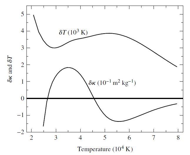
Fig. 10.7 Variations in the temperature and opacity throughout an RR Lyrae stellar model at the time of maixmum compression. In the \({\rm He\ II}\) partial ionization zone (\(T\approx 4\times 10^4\ {\rm K}\)), \(\delta \kappa > 0\) and \(\delta T\) is reduced. Figure credit: Carroll & Ostlie (2007).

Similarly, during expansion, the temperature does not decrease as much as expected since the ions now recombine with electrons and release energy. When the density term in the Kramers law dominates, the opacity decreases with decreasing density during the expansion. This layer of the star can absorb heat during compression, be pushed outward to release the heat during expansion, and fall back again to begin another cycle. The opacity mechanism is called the \(\kappa\)-mechanism.

In a partial ionziation zone, the \(\kappa\)-mechanism is reinforced by the tendency of heat to flow into the zone during compression because its temperature has increased less than the adjacent stellar layers. This effect is called the \(\gamma\)-mechanism, after the smaller ratio of specific heates caused by the increased values of \(C_p\) and \(C_V\).

Partial ionization zones are the pistons that drive the oscillations of stars, where they modulate the energy flow through the stellar layers and are the direct cause of stellar pulsation.

10.2.7. The Hydrogen and Helium Partial Ionization Zones

In most stars, there are two main ionization zones.

• The first is a broad zone where both the ionization of neutral hydrogen and the first ionization of helium occur in layers with a characteristic temperature of \(1-1.5 \times 10^4\ {\rm K}\). These layers are called the hydrogen partial ionization zone.

• The second, deeper zone involves the second ionization of helium, which occurs at a characteristic temperature of \(4\times 10^4\ {\rm K}\). Unsurpisingly, this is called the \({\rm He\ II}\) partial ionization zone.

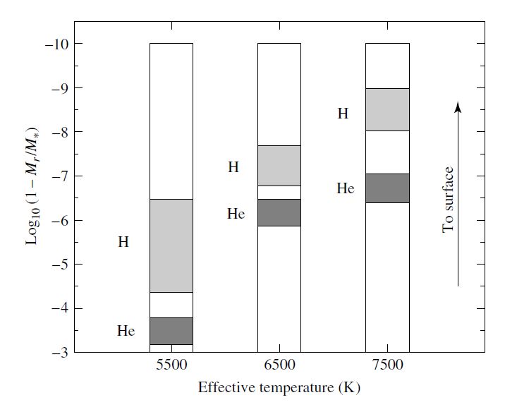
Fig. 10.8 Hydrogen and helium ionization zones in stars of different temperatures. For each point in the star, the vertical axis displays the logarithm of the fraction of the star’s mass that lies above that point. Figure credit: Carroll & Ostlie (2007).

The location of these ionization zones with the star determines its pulsational properties.

• If the star is too hot (\(7500\ {\rm K}\)), the ionization zones will be very near the surface. At this position, the density is quite low, and there is not enough mass available to drive the oscillations effectively. This accounts for the hot blue edge of the instability strip on the H-R diagram.

• In a cooler star (\(6500\ {\rm K}\)), the characteristic temperatures of the ionzation zones are found deeper in the star. There is more mass for the ionization zone “piston” to push around, and the first overtone mode may be excited.

• In a still cooler star (\(5500\ {\rm K}\)), the ionization zones occur deep enough to drive the fundamental mode of pulsation.

However, if a star’s surface temperature is too low, the onset of efficient convection in its outer layers may dampen the oscillations. The transport of enerby via convection is more effective when the star is compressed, and the convecting stellar material may lose heat at the minimum radius. This would overcome the damming up of heat by the ionization zones and quench the pulsation of the star. The cool red edge of the instability strip is the result of the damping effect of convection.

Detailed numerical calculations demonstrate a good agreement for the location of the instablilty strip on the H-R diagram. These computations show that it is the \(\rm He\ II\) partial ionization zone that is primarily responsible for driving stellar oscillations within the instability strip. If the effect of the helium ionization is artificially removed, then the model stars will not pulsate.

The hydrogen ionization zone plays a more subtle role. As a star pulsates, the hydrogen ionization zone moves toward or away from the surface as the zone expands and contracts in response to the changing temperature of the stellar gases. The star is brightest when the least mass lies between the hydrogen ionziation zone and the surface.

As a star oscillates, the location of an ionization zone changes with respect to both its radial position \(r\) and the mass enclosed \(M_r\). The luminosity incident on the bottom of the hydrogen ionization zone is a maximum at minimum radius, but this propels the zone outward (through mass) most rapidly at that instant. The emergent luminosity is greatest after minimum radius, when the zone is nearest the surface. The delaying action (of the hydrogen partial ionization zone) produces the phase lag observed for classical Cepheids and RR Lyrae stars.

The mechanisms repsonsible for the pulsation of stars outside the instability strip are not always well understood. The long-period variables (LPVs) are red supergiants with huge, diffuse convective envelopes surrounding a compact ocre. Their spectra are dominated by molecular absorption lines and emission lines that reveal the existence of atmospheric shock waves and significant mass loss.

10.2.8. \(\beta\) Cephei Stars and the Iron Opacity “Bump”

The \(\beta\) Cephei stars pose another interesting challenge, where they are located in the upper left-hand side of the H-R diagram (i.e., very hot and luminous). \(\beta\) Cepheis are early B stars with effective temperatures from \(2-3 \times 10^4\ {\rm K}\) and typically luminosity classes of III, IV, and V.

Given their high effective temperatures, hydrogen is completely ionized, and the helium ionization zone is too near the surface to effectively drive pulsations. After many years, it was realized tha the \(\kappa\) and \(\gamma\) mechanisms are still active in \(\beta\) Cephei stars, but the element responsible for the driving is iron.

The larger number of absorption lines in the spectrum of iron implies that iron contributes significantly to stellar opacities at temperatures near \(10^5\ {\rm K}\). This effect can be seen in the “iron bump” above \(10^5\ {\rm K}\) in the plot of opacity. The depth of this iron ionization region is sufficient to produce net positive pulsational driving in these stars.

10.3. Modeling Stellar Pulsation

10.3.1. Nonlinear Hydrodynamic Models

A pulsating star is not in hydrostatic equilibrium, where a more general set of equations is employed that takes the oscillation of mass shells into account. For example, Newton’s second law

\[\begin{align*} \rho \frac{d^2 r}{dt^2} = -\frac{GM_r \rho}{r^2} - \frac{dP}{dr}, \end{align*}\]

must be used for hydrostatic equilibrium. But the differential equations describing nonequilibrium mechanical and thermal behavior of a star are needed. Such equations may be replaced by difference equations and solved numerically. The model star is displaced from its equilibrium configuration and “released” to begin its oscillation. The mass shells expand and contract, pushing against each other as they move.

If the conditions are right, the ionization zones in the model star will drive the oscillations, and the pulsation amplitude will slowly increase; otherwise the amplitude will fade away. Computer programs that carry out these calculations have been successful in modeling the details observed in the light and radial velocity curves of Cepheid variables.

The main advantage of the preceeding approach is that it is a nonlinear calculation, capable (in principle) of modeling the complexitites of large pulsation amplitudes and reproducing the nonsinusoidal shape of actual light curves. One disadvantage lies in the computer resources required:

• The process requires a significant amount of CPU time andmemory.

• Many (sometimes thousands of) oscillations must be evaluated before the model settles down into a well-behaved periodic motion.

• Even more periods may be required for the model to reach its limit cycle, when the pulsation amplitude has reached its final value.

In some cases the computer simulations of certain classes of pulsating stars may never attain a truly periodic solution but exhibit chaotic behavior instead, as observed in some real stars.

A second disadvantage of nonlinear calulations lies in the challenges involved in accurately convering models at each time step. Numerical instabilities in the nonlinear equations can cause calculations to lead to unphysical solutions. This is particularly true when theories of time-dependent convection are required for red giants and supergiants.

10.3.2. Linearizing the Hydrodynamic Equaitons

An alternative to the nonlinear approach is to linearize the differential equaitons by considering only small-amplitude oscillations. This is done by writing every variable in the differential equations as an equilibrium value plus a small change due to the pulsation (i.e., a perturbative method). For example, the pressure \(P\) would be written as \(P = P_o + \delta P\), where \(P_o\) is the pressure in a mass shell of the equilibrium model, and \(\delta P\) is the small change in pressure that occurs as that mass shell moves in the oscillating model star.

Note that \(\delta P\) varies in time, while \(P_o\) is a constant. When the variables written in this manner are inserted into the differential equations, the terms containing only equilibrium quantities cancel, and terms that involve powers greater than second order (i.e., greater than \((\delta P)^2)\) may be discarded because they are negligibly small. The resulting linearized differential equations and their associated boundary conditions (also linearized) are similar to the equations for a wave on a string or in an organ pipe.

Only certain standing waves with specific periods are permitted, where the pulsation modes of the star are clearly identified. The equations are sufficiently complicated that the motion of the star is forced to be sinusoidal, and the limiting value of the pulsation amplitude cannot be determined. Modeling the complexities of the full nonlinear behavior of the stellar model is thus sacrificed.

Exercise 10.1

Consider an unrealistic (but very instructive) model of a pulsating star called a one-zone model. It consists of a central point mass equal to the entire mass of the star \(M\), surrounded by a single thin, spherical shell of mass \(m\) and radius \(R\) that represents the surface layer of the star. The interior of the shell is filled with a massless gas of pressure \(P\) whose function is to support the shell against gravity.

Determine the pulsation period \(\Pi\) using the perturbation approximation.

First, we apply Newton’s second law for a shell as

(10.8)\[\begin{align} \rho \frac{d^2 r}{dt^2} &= -\frac{GM_r \rho}{r^2} - \frac{dP}{dr}, \\ \frac{m}{V} \frac{d^2 R}{dt^2} &= -\frac{GM}{R^2}\frac{m}{V} + \frac{P}{R}, \\ m \frac{d^2 R}{dt^2} &= -\frac{GMm}{R^2} + PA, \\ m \frac{d^2 R}{dt^2} &= -\frac{GMm}{R^2} + 4\pi R^2 P. \end{align}\]

For the equilibrium model, the left-hand side of this equation is zero, where

(10.9)\[\frac{GMm}{R_o^2} = 4\pi R_o^2 P_o.\]

The linearization is accomplished by writing the star’s radius and pressure as

(10.10)\[\begin{align} R &= R_o + \delta R, & \text{and} \\ P &= P_o + \delta P, & \end{align}\]

which we then insert into our result from Newton’s second law. This gives

(10.11)\[\begin{align} m \frac{d^2}{dt^2}\left[R_o + \delta R\right] &= -\frac{GMm}{\left(R_o + \delta R\right)^2} + 4\pi \left(R_o + \delta R\right)^2 (P_o + \delta P). \end{align}\]

Using the first-order approximation

\[\begin{align*} \frac{1}{\left(R_o + \delta R\right)^2} &= \frac{1}{R_o^2\left(1 + \frac{\delta R}{R_o}\right)^2}, \\ &= \frac{1}{R_o^2}\left(1 + \frac{\delta R}{R_o}\right)^{-2}, \\ &\approx \frac{1}{R_o^2}\left(1 - 2\frac{\delta R}{R_o}\right) \end{align*}\]

and keeping only those terms involving the first powers of the deltas results in

(10.12)\[\begin{align} m \frac{d^2 (\delta R)}{dt^2} &= -\frac{GMm}{R_o^2} + 2\frac{GMm}{R_o^3} + 4\pi R_o^2 P_o + 8\pi R_o P_o \delta R + 4\pi R_o^2 \delta P, \end{align}\]

where \(d^2 R_o/dt^2 = 0\) is used for the equilibrium model. Also in the equlibrium model (Eq. (10.9)), the first and third terms on the right-hand side cancel, which leaves

(10.13)\[m \frac{d^2 (\delta R)}{dt^2} = 2\frac{GMm}{R_o^3} + 8\pi R_o P_o \delta R + 4\pi R_o^2 \delta P.\]

This is the linearized version of Newton’s second law for our one-zone model.

To reduce from two variables (\(\delta R\) and \(\delta P\)) to one, we assume that the oscillations are adiabatic. As a result, the pressure and volume are related by the adiabatic relation \(PV^\gamma =\ \text{constant}\), where \(\gamma\) is the ratio of specific heats of the gas. The volume of the one-zone model is just the volume of a sphere (\(4/3\pi R^3\)), the adiabatic relation becomes \(PR^{3\gamma} =\ \text{constant}\). Then the linearized version is found as (see HW)

(10.14)\[\frac{\delta P}{P_o} = -3\gamma \frac{\delta R}{R_o}.\]

Using this equation, \(\delta P\) can be eliminated from Eqn. (10.13). In addition, the \(8\pi R_o P_o\) can be replaced by \(2GMm/R_o^3\) using Eqn. (10.9). Then, the mass \(m\) of the shell cancels, which leaves the linearized equation for \(\delta R\),

(10.15)\[\frac{d^2(\delta R)}{dt^2} = -(3\gamma - 4)\frac{GM}{R_o^3}\delta R.\]

If \(\gamma > 4/3\), the above relation reduces to the equation for simple harmonic motion, which has a solution \(\delta R = A \sin{(\omega t)}\), where \(A\) represents the pulsation amplitude and \(\omega\) is the angular pulsation frequency. Substituting this particular solution into Eqn. (10.15) results in

(10.16)\[\begin{align} \omega^2 &= (3\gamma - 4)\frac{GM}{R_o^3}. \end{align}\]

From this, we can determine the pulsation period of the one-zone model as

(10.17)\[\begin{align} \Pi & = 2\pi/\omega, \\ &= \frac{2\pi}{\sqrt{\frac{4\pi}{3}G\rho_o (3\gamma - 4)}}, \end{align}\]

where \(\rho_o\) is the average density of the equilibrium model. For an ideal monatomic gas, \(\gamma = 5/3\). Except for factors of order unity, this is the same as our earlier estimate (Eqn. (10.7)) when we considered the time required for a sound wave to cross the stellar diameter.

Note

In the above example, the approximations that the pulsation of the one-zone model was linear and adiabatic were used to simplify the calculation. Note that the pulsation amplitude \(A\) canceled in this example. The inability to calculate this amplitude is an inherent drawback of the linearized approach to pulsation.

10.3.3. Nonlinear and Nonadiabatic Calculations

Because no heat is allwed to enter (or leave) the layers of a stellar model in an adiabitic analysis, the oscillation amplitude remains constant. However, astronomers need to know which modes will grow and which will decay away. This calculation must include the physics involved in Eddington’s valve mechanism.

The equations describing the heat transfer and radiation through the stellar layers must be incorporated in a nonadiabatic computation. These nonadiabatic expressions may also be linearized and solved to obtain the periods and growth rates of the individual modes. However, a more sophisticated (and costly) nonlinear, nonadiabatic calculation is needed to reproduce the complicated light and radial velocity curves for some variable stars. As a result, such computations are performed numerically.

10.3.4. Dynamical Stability

Equation (10.15) provides a very important insight into the dynamical stability of a star. If \(\gamma < 4/3\), then the right-hand side is positive. The solution changes from a sinusoidal function to a decaying exponential, or \(\delta R = Ae^{-\kappa t}\), where \(\kappa^2\) is the same as \(\omega^2\). Instead of pulsating, the star collapses if \(\gamma < 4/3\). The increase in gas pressure is not enough to overcome the inward pull of gravity and push the mass shell back out again, which results in a dynamically unstable model.

For the case of nonadiabatic oscillations, the time dependence of the pulsation is usually taken to be the real part of \(e^{i\sigma t}\), where \(\sigma\) represents the complex frequency \(\sigma = \omega + i\kappa\). in this expression, \(\omega\) is the pulsation frequency and \(\kappa\) is a stability coefficient. The pulsation amplitude is then proportional to \(e^{-\kappa t}\), and \(\kappa^{-1}\) is the characteristic time for growth or decy of the oscillations.

10.4. Nonradial Stellar Pulsation

As some stars pulsate, their surfaces excecute a more complicated type of nonradial motion in which some regions of its surface expand while other areas contract.

10.4.1. Nonradial Oscillations and Spherical Harmonic Functions

The python code produces a figure shoing the angular patterns for several nonradial modes. If the stellar surface is moving outward within the red regions, then it is moving inward within the blue regions. Scalar quantitites, such as the change in pressure \(\delta P\), follow the same pattern with positive values in some areas and negative values in others.

import matplotlib
import matplotlib.pyplot as plt
from matplotlib import cm, colors
import numpy as np
from scipy.special import sph_harm

phi = np.linspace(0, np.pi, 100)
theta = np.linspace(0, 2*np.pi, 100)
phi, theta = np.meshgrid(phi, theta)

# The Cartesian coordinates of the unit sphere
x = np.sin(phi) * np.cos(theta)
y = np.sin(phi) * np.sin(theta)
z = np.cos(phi)

sph_idx = [(0,0),(2,2),(1,-1),(2,-1),(1,0),(2,0)]

width = 2.5
cmap = cm.bwr
my_cmap = matplotlib.colormaps.get_cmap(cmap)
# Set the aspect ratio to 1 so our sphere looks spherical
fig = plt.figure(figsize=(2*width,3*width),dpi=150)
ax_list = []
for i in range(1,7):
    ax = fig.add_subplot(3,2,i, projection='3d',aspect='equal')
    if i == 1:
        # Plot the surface
        ax.plot_surface(x, y, z, color=my_cmap(0.5))
        label = '$\ell$ = %i, $m$ = %i' % (0,0)
    else:
        l,m = sph_idx[i-1]
        # Calculate the spherical harmonic Y(l,m) and normalize to [0,1]
        fcolors = sph_harm(m, l, theta, phi).real
        fmax, fmin = fcolors.max(), fcolors.min()
        fcolors = (fcolors - fmin)/(fmax - fmin)
        ax.plot_surface(x, y, z, rstride=1, cstride=1, facecolors=my_cmap(fcolors))
        label = '$\ell$ = %i, $m$ = $\pm$%i' % (l,np.abs(m))
    ax.text(-0.8,0,1.2,label,None)
    # Turn off the axis planes
    ax.set_axis_off()
    ax_list.append(ax)
fig.subplots_adjust(hspace=-0.35,wspace=-0.15)
fig.savefig("Sph_Harm.png",bbox_inches='tight',dpi=150)

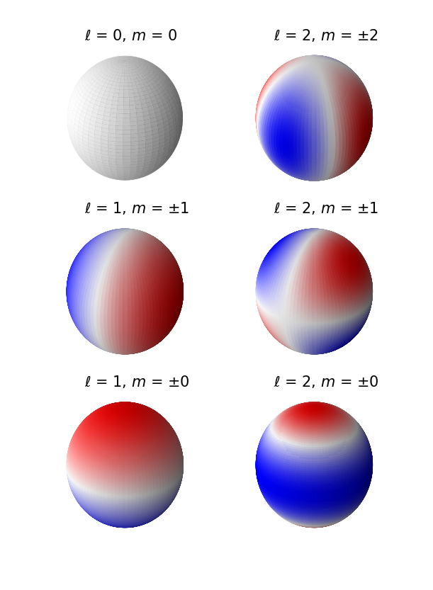
Formally, these patterns are described by the real parts of the spherical harmonic functions \(Y^m_\ell(\theta,\phi)\), where \(\ell \ge 0\) (an integer) and \(m\) is also an integer between \(-\ell\) and \(+\ell\). There are \(\ell\) nodal circles (where \(\delta r = 0\)), with \(|m|\) of these circles passing through the poles of the star and the remaining \(\ell - |m|\) nodal circles parallel to the star’s equator. If \(\ell = m = 0\), the n the pulsation is purely radial.

A few examples of \(Y^m_\ell(\theta,\phi)\) functions are:

\[\begin{align*} Y^0_0(\theta,\phi) &= K^0_0, & Y^0_2(\theta,\phi) &= K^0_2\ \left(3\cos^2{\theta} -1\right), \\ Y^0_1(\theta,\phi) &= K^0_1\ \cos{\theta}, & Y^{\pm 1}_2(\theta,\phi) &= K^{\pm 1}_2\ \sin{\theta}\cos{\theta}e^{\pm i\phi}, \\ Y^{\pm 1}_1(\theta,\phi) &= K^{\pm 1}_1\ \sin{\theta}e^{\pm i\phi}, & Y^{\pm 2}_2(\theta,\phi) &= K^{\pm 2}_2\ \cos^2{\theta}e^{\pm 2i\phi}, \\ \end{align*}\]

where the \(K^{\pm m}_\ell\) are normalization constants and \(i\) is the imaginary number.

Note

Recall from Euler’s formula that \(e^{\pm mi\phi} = \cos(m\phi) \pm i\sin{m\phi}\). Thus the real part of \(e^{\pm mi\phi}\) is just \(\cos(m\phi)\).

The patterns for nonzero \(m\) represent traveling waves that move across the star parallel to its equator. The time required for the waves to travel around the star is \(|m|\) times the star’s pulsation period.

It is important to note that the star itself may not be rotating at all. Just as water waves may travel across the surface of a lake without the water itself making the trip, these traveling waves are distrubances that pass through the stellar gases.

10.4.2. The \(p\) and \(f\) Modes

In The Physics of Stellar Pulsation, the radial pulsation of stars was attributed to standing sound waves in the stellar interior. For the case of nonradial oscillations, the sound waves can propogate horizontally, as well as radially, to produce waves that travel arount the star. Because pressure provides the restoring force for sound waves, these nonraidal oscillations are called \(p\)-modes.

A complete description of a \(p\)-mode requires specificaation of its radial and angular nodes. For example, a \(p_2\) mode can be considered a nonradial analog of a radial second overtone mode. The \(p_2\) mode (with \(\ell = 4\) and \(m=3\)) has two radial nodes between the center and the surface, and its angular pattern has four nodal lines, three through the poles and one parallel to the equator.

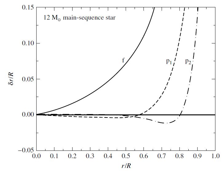
Fig. 10.9 Nonradial \(p\)-modes with \(\ell = 2\). The waveforms have been arbitrarily scales so that \(\delta r/R = 1\) a the star’s surface. Figure credit: Carroll & Ostlie (2007).

Figure 10.9 shows two \(p\)-modes for a \(12\ M_\odot\) main-sequence star model. Also shown is the \(f\)-mode, which is similar to a surface gravity wave due to the rapid rise in amplitude with radius. The frequency of the \(f\)-mode is intermediate between the \(p\)- and \(g\)-modes. There is no radial analog for the \(f\)-mode.

10.4.3. The Acoustic frequency

An estimate of the angular frequency of a \(p\)-mode can be made from the time for a sound wave to travel one horizontal wavelenth, from one angular node line to the nest. This horizontal wavelength is given by

(10.18)\[\begin{align} \lambda_h = \frac{2\pi r}{\sqrt{\ell(\ell +1)}}, \end{align}\]

where \(r\) is the radial distance from the center of the star. The acoustic frequency at this depth in the star is then defined as

\[\begin{align*} S_\ell = \frac{2\pi}{\text{time for sound to travel }\lambda_h}, \end{align*}\]

which can be written as

(10.19)\[\begin{align} S_\ell &= 2\pi \left[\frac{v_s}{2\pi r/\sqrt{\ell(\ell+1)}}\right], \\ &= \sqrt{\frac{\gamma P}{\rho}}\frac{\sqrt{\ell(\ell + 1)}}{r}, \end{align}\]

where \(v_s\) is the adiabatic sound speed (see The Period-Density Relation).

Because the sound speed is proportional to the square root of the temperature (from the ideal gas law; \(P/\rho \propto T\)), the acoustic frequency is large in the deep interior of the star and decreases with increasing \(r\). The frequency of a \(p\)-mode is determined by the average value of \(S_\ell\), with the largest contributions to the average coming from the stellar regions where the oscillations are most energetic.

In the absence of rotation, the pulsation period depends only on the number of radial nodes and the integer \(\ell\). The period is independent of \(m\) because with no rotation there are no well-defined poles or equator; thus \(m\) has no physical significance.

In the case with rotation, the rotation itself defines the poles and equator, and the pulsation frequencies for modes with different values of \(m\) becomes separated or split as the traveling waves move either with or against the rotation, where the sign of \(m\) determines the direction in which the wave moves around the star.

The amount by which the pulsation frequencies are split depends on the stellar angular rotation frequency \(\Omega\), whith the rotationally produced shift in frequency proportional to \(m\Omega\) for the simple case of uniform rotation.

10.4.4. The \(g\) modes

Just as pressure supplies the restoring force for compression and expansion of the \(p\)-mode sound waves, gravity is the source of the restoring force for the nonradial oscillations called \(g\)-modes. The \(g\)-modes are produced by internal gravity waves.

These wave involve a “sloshing” back and forth of the stellar gases, which is ultimately connected to the buoyancy of stellar material. Because “sloshing” cannot occur for purely radial motion, the are no radial analogs for the \(g\)-modes.

10.4.5. The Brunt-Väisälä (Buoyancy) Frequency

To better understand the \(g\)-modes, consider a small bubble of stellar material that is displaced upward from its equilibrium position by an amount \(dr\). We wll assume that the motion occurs

1. slow enough for the pressure in the bubble, \(P^b\), is always equal to the pressure of its surroundings, \(P^s\); and

2. rapid enough so that no heat is exchanged between the bubble an dits surroundings (i.e., adiabatic).

If the density of the displaced bubble is greater than the density of its new surroundings, the bubble will fall back to its original position. The net restoring force per unit volume on the bubble is the difference between the upward buoyant force (i.e., Archimedes’ law) and the downward gravitational force at its final location:

\[ f_{\rm net} = \left( \rho_f^s - \rho_f^s\right)\ g, \]

where \(g\) represents the local gravity (\(GM_r/r^2\)). Using a Taylor expansion for the densitites about their initial positions in

\[f_{\rm net} = \left[\left( \rho_i^s + \frac{d\rho^s}{dr}dr\right) - \left( \rho_i^b + \frac{d\rho^b}{dr}dr\right)\right]\ g. \]

The initial densities of the bubble and its surroundings are the same (\(\rho_i^s = \rho_i^b\)) and after canceling terms, leaves

\[f_{\rm net} = \left(\frac{d\rho^s}{dr} - \frac{d\rho^b}{dr}\right)\ g\ dr. \]

Because the motion of the bubble is adiabatic (and considering the conditions for convection), the \(d\rho^b/dr\) can be replaced to get

\[ f_{\rm net} = \left(\frac{d\rho^s}{dr} - \frac{\rho^b}{\gamma P_i^b}\frac{dP^b}{dr}\right)\ g\ dr. \]

Actually, all of the \(b\) superscripts can be changed to \(s\) because the initial densities are equal. Using our first assumption, the pressures inside and outside the bubble are always the same. Thus all quantities in refer to the stellar material surrounding the bubble, which allows us to drop the subscripts/superscipts and results in

(10.20)\[\begin{split}f_{\rm net} &= \left(\frac{d\rho}{dr} - \frac{\rho}{\gamma P}\frac{dP}{dr}\right)\ g\ dr\\ &= A \rho g\ dr.\end{split}\]

The \(A\) represents the difference in the rate of change for the pressure and density (see Eq. (7.57)).

If \(A>0\), the net force has the same sign as \(dr\) and the bubble will contiune to move away from its equilibrium position. This is the condition necessary for convection to occur.

However, if \(A<0\), then the net force will be in an opposite direction relative to the displacement and the bubble will be pushed back toward its equilibrium position. In this case, the result of Eq. (10.20) has the form of Hooke’s law with the restoring force proportional to the displacement. We should expect that the bubble will oscillate about its equilibrium position with simple harmonic motion when \(A<0\).

Dividing the force per unit volume \(f_{\rm net}\) by the mass per unit volume \(\rho\), gives the force per unit mass (or acceleration): \(a = f_{\rm net}/\rho = Ag\ dr\). As a result, we have

\[ a = -N^2 dr = Ag\ dr, \]

where \(N\) represents the angular frequency of the bubble about its equilibrium position and is called the **Brunt-Väisälä frequency$$ or the bouyant frequency. More explicitly,

(10.21)\[\begin{align} N &= \sqrt{-Ag}, \\ &= \sqrt{\frac{\rho}{\gamma P}\frac{dP}{dr} - \left(\frac{d\rho}{dr}\right)\ g}. \end{align}\]

The bouyancy frequency is zero at the stellar center (where \(g=0\)) and at the edges of the convection zones (where \(A=0\)).

10.4.6. The \(g\) and \(p\) Modes as Probes of Stellar Structure

The sloshing effect of neighboring regions of the star produces the internal gravity waves that are responsible fo rthe \(g\)-modes of a nonradially pulsating star. The frequency of a \(g\)-mode is determined by the value of \(N\) averaged across the star.

\(f\)-modes and \(g\)-modes each produce different profiles for how material moves radially within a star. This makes them useful to astronomers attempting to study stellar interiors. The \(g\)-modes involve significant movement of the stellar material deep within the star, while the \(p\)-mode’s motion are confined to the stellar surface. Thus, \(g\)-modes provide a view into the very heart of a star, while \(p\)-modes present the conditions in the surface layers.

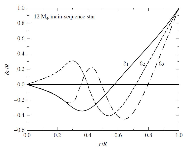
Fig. 10.10 Nonradial \(g\)-modes with \(\ell = 2\). The waveforms have been arbitrarily scales so that \(\delta r/R = 1\) a the star’s surface. Figure credit: Carroll & Ostlie (2007).

10.5. Helioseismology and Asteroseismology

Nonradial pulsation is a the heart of a science called helioseismology. A typical solar oscillation mode has a very low amplituded, with a surface velocity of only \(10\ {\rm cm/s}\) or less, and a luminosity variation \(\delta L/L_\odot\) of only \(10^{-6}\). With an incoherent superposition of roughly ten million modes rippling through the Sun’s surface and interior, our star is “ringing” like a bell.

10.5.1. The Five-Minute Solar Oscillations

The oscillations observed on the Sun have modes with periods from \(3-8\) minutes and very short horizontal wavelengths (\(\ell\) ranging up to 1000 or more). These so-called five-minute oscillations are \(p\)-modes. The five-minute \(p\)-modes are concentrated below the photosphere within the Sun’s convection zone, where \(g\)-modes are located deep in the solar interior. By studying these \(p\)-mode oscillations, astronomers have been able to gain new insights in the structure of the Sun in these regions.

10.5.2. Differential Rotation and the Solar Convection Zone

Based on studies of helioseismology (combined with detailed stellar evolution calculations), we know the base of the solar convection zone lies at \(0.714\ R_\odot\) with a temperature of about \(2.18 \times 10^6\ {\rm K}\). The rotational splitting observed for \(p\)-mode frequencies indicates that differential roation observed at the Sun’ surface decreases slightly down through the convection zone.

Those \(p\)-modes with shorter horizontal wavelengths (larger \(\ell\)) do not penetrate the convection zone as deeply, so the difference in rotational frequency splitting with \(\ell\) reveals the depth dependence of the rotation. The measured depth dependence of the differential rotation comes from the dependence on the rotational frequency splitting on \(m\).

Below the convection zone, the equatorial and polar rotation rates converge to a single value at \(r/R_\odot \approx 0.65\). To convert the Sun’s magnetic field from a poloidal to a toroidal geometry a change in the rotation rate with depth is needed. The Sun’s magnetic dynamo is probably seated in the tachocline at the interface between the radiation and convection zones.

10.5.3. Probing the Deep Interior

Astronomers had more difficulty using the solar \(g\)-modes as a probe of the Sun’s interior because they dwell beneath the convection zone, where their amplitudes are significantly diminished at the Sun’s surface. Here is an astrobites article summarizing a recent attempt to measure the \(g\)-modes indirectly. However, a definitive measurement remains hotly debated.

10.5.4. Driving Solar Oscillations

The question of the mechanism responsible for driving the solar oscillations has not been conclusevely answered. Our main-sequence Sun lies beyond the red edge of the instability strip on the H-R diagram. Therefore, Eddington’s valve mechanism cannot be responsible for the solar oscillations. However, the timescale for convection near the top of the convection zone is a few minutes, and it is strongly suspected that the \(p\)-modes are driven by tapping in to the turbulent energy of the convection zone itself, where the \(p\)-modes are confined.

10.5.5. \(\delta\) Scuti Stars and Rapidly Oscillating Ap Stars

The techniques of helioseismology can be applied to other stars to become asteroseismology, where astronomers study the pulastion modes of other stars in order to investigate their internal structures, chemical compositions, rotation, and magnetic fields.

\(\delta\) Scuti stars are Pop I main-sequence and giant stars within the spectral type range \(\rm A-F\). They tend to pulsate in low-overtone radial modes and in low-order \(p\)-modes (and possibly \(g\)-modes). The amplitudes of \(\delta\) Scutis are fairly small, ranging from a few millimagnitudes to roughly 0.8 mag. Population II subgiants also exhibit radial and nonradial oscillations, which are known as SX Phoenicis stars.

The rapidly oscillating Ap stars (\(\rm roAp\)) are found in the same portion of the H-R diagram as the \(\delta\) Scuti stars. These stars have peculiar surface chemical compositions (hence the “p” designation), are rotating, and have strong magnetic fields. The unusual chemical composition is likely du to the settling of heavier elements, similar to the elmenetal diffusion that has occured near the surface of the Sun.

Some elements may have been eleveated in the atmosphere if they have a significant number of absorption lines near the peak of the star’s blackbody spectrum. These atoms preferentially absorb photons that impart a net upward momentum. If the atmosphere is sufficiently stable against turbulent motions, some of these atoms will tend to drift upward.

\(\rm roAp\) stars have very small pulsation amplitutdes of less than 0.016 mag. It appears that they primarly pulsate in higher-order \(p\)-modes and that the axis for the pulsation is aligned with the magnetic field axis, which is tilted relative to the roation axis. \(\rm roAp\) star are among the most well-studied of main-sequene stars other than the Sun, but the pulsation driving mechanism still remains in question.

10.6. Homework

Problem 1

Derive Eqn. (10.14) by linearizing the adiabatic relation \(PV^\gamma =\ \text{constant}\).

10.7. Additional Resources

• Notes on radial stellar pulsations by Gillian Knapp @ Princeton

• Notes on Stellar Oscillations by Mike Montgomery at UTexas Austin