8. The Interstellar Medium and Star Formation#
8.1. Interstellar dust and gas#
8.1.1. The Interstellar Medium#
The evolution of stars is a cyclic process, where a star is born out of gas and dust that exists between the stars (i.e., interstellar medium or ISM). During a star’s lifetime, much of that material may return to the ISM through stellar winds or explosive events. The next generation of stars can then form from the ashes, which are processed by the nuclear fusion within the deep interiors of stars. Thus it’s important to study the nature of the ISM so that we can better understand stellar evolution.
The ISM is an enormous and complex environment that provides a laboratory for testing our basic understanding of astrophysics (i.e., its the testbed to develop sensible initial conditions for stellar models). The ISM interacts with the stellar environment through shocks and galactic magnetic fields that extend into interstellar space. As a result, modeling the ISM requires detailed modeling of the magnetohydrodynamics (MHD) equations.
8.1.2. Interstellar Extinction#
On a dark night (far from city lights), some of the dust clouds within the Milky Way Galaxy can be found because they obscure regions of sky that would otherwise be populated with stars. These dark regions are not devoid of stars, but the intervening dust blocks the background starlight. Dust that blocks starlight is due to the combined effet of scattering and absorption, which is called interstellar extinction. The apparent magnitude is a measure of how bright a star appears and if it is dimmed by intervening dust, the distance modulus equation must be modified appropriately. In a given wavelength band centered on \(\lambda\), we have
which is a modified version of the distance modulus equation with a correction factor \(A_\lambda>0\) that adjusts for the interstellar extinction along the line of sight. The extinction magnitude \(A_\lambda\) is positive because it always acts to dim objects along the magnitude scale. If \(A_\lambda\) is large enough, a star can fall behind the limiting magnitude of the background sky for the naked eye or a telescope. This is the cause for the dark bands running through the Milky Way.

Fig. 8.1 Dust clouds obscuring the light in the center of NGC 281. (Image Credit: NASA, ESA, and the Hubble Heritage TEam (STScI/AURA); P. McCullough (STScI))#

Fig. 8.2 An interstellar cloud containing significant amounts of dust along with the gas (a dust cloud) can both scatter and absorb light that passes through it. (Carroll & Ostlie (2007))#
The extinction magnitude \(A_\lambda\) is related to optical depth (recall that the gas below the photosphere is also invisible) measured back along the line of sight. The fractional change in the intensity of light decreases exponentially by,
which is normalized by the expected light intensity without interstellar extinction. The optical depth correlates with the change in magnitude through the fractional change in light intensity (see the magnitude scale), or
The change in apparent magnitude is simply the extinction magnitude \(A_\lambda\), or
which restates that the change in magnitude due to extinction is approximately equal to the optical depth along the line of sight. The optical depth through the cloud is
which depends on the number density of scattering dust grains \(n_d(s^\prime)\) and the scattering cross section \(\sigma_\lambda\). If the scattering cross section is constant along the line of sight, then
and the dust grain column density \(N_d\) represents the number of scattering dust particles in a thin cylinder with a cross section of 1 \({\rm m^2}\) stretching from the observer to the star. The magnitude of extinction depends on the amount of interstellar dust that the light passes through.
8.1.3. The Mie Theory#
Assuming that the dust particles are spherical with a radius \(a\), the geometrical cross-section of the dust particle is \(\sigma_g = \pi a^2\). The dimensionless extinction coefficient \(Q_\lambda\) is then defined as
where the extinction coefficient \(Q_\lambda\) depends on the composition of the dust grains. When the wavelength of the light is similar to the size of the dust grains, then \(Q_\lambda \sim a/\lambda\), implying that
The extinction coefficient \(Q_\lambda\) goes to zero when the wavelength \(\lambda\) is large compared to \(a\). Conversely, the extinction coefficient \(Q_\lambda\) approaches a constant (independent of \(\lambda\)) when the wavelength \(\lambda\) is very small compared to \(a\) or
Note
Gustav Mie made similar assumptions concerning dust particles in 1908 and showed the relationship between the scattering cross section \(\sigma_\lambda\) and the radius of a dust grain.
These limiting cases can be understood by analogy with the waves on the surface of a lake. If the size of the surface waves (i.e., wavelength) is much larger than an object in their way, then the waves pass by almost completely unaffected \((\sigma_\lambda \sim 0)\). However, if the object (e.g., an island) is large compared to the waves, then they are simply blocked. The only waves that pass by the large object are those that miss it altogether. The light we detect from a dust cloud is the light that passes between the dust particles.
The extinction magnitude \(A_\lambda\) is clearly wavelength-dependent, where longer wavelengths (redder light) are not scattered as strongly as shorter wavelengths (bluer light). The starlight that passes through is preferentially red, or reddened, as the blue light is removed. This interstellar reddening causes stars to appear redder, where we might infer them to be cooler through Wien’s law. Fortunately, we can carefully analyze the star’s spectrum (i.e., absorption and emission lines) to detect the change.
Strongly scattered blue light can leave the cloud in any direction, where a bright star behind a cloud casts a blue reflection nebula for observers that are not along the line of sight (e.g., the Pleiades). This process is analogous to Rayleigh scattering, which produces a blue sky on Earth. The difference between Mie scattering and Rayleigh scattering is that the scattering particles are much smaller than the wavelength of visible light in Rayleigh scattering and leads to \(\sigma_\lambda \propto \lambda^{-4}\).
Exercise 8.1
A star is found to be dimmer than expected at 550 nm by 1.1 magnitudes in the visual (i.e., \(A_V = 1.1\)). If \(Q_{550}=1.5\) and the radius of the dust grains are 0.2 \({\rm \mu m}\), estimate the average density \(\overline{n}\) of the material between the star and Earth. The star is 0.8 kpc from Earth.
The extinction magnitude \(A_\lambda\) is related to the optical depth \(\tau_\lambda\) by a faction of 1.086, where \(\tau_{550} = 1.1/1.086 \simeq 1\). Given the radius of the dust grains \((a = 0.2\,{\rm \mu m})\) and the extinction coefficient \(Q_{550} = 1.5\) we have,
The column density of the dust along the line of sight is
and the column density is the integrated particle density across the distance to the star. Then we have,
import numpy as np

pc = 3.0857e16 #1 pc in meters
a = 0.2e-6 #radius of the dust grains converted to meters
A_lambda = 1.1
Q_lambda = 1.5

tau_550 = A_lambda/1.086
sigma_550 = 1.5*np.pi*a**2
print("The scattering cross section for the grain is %1.1e m^2." % sigma_550)

N_d = tau_550/sigma_550
print("The column density of the dust along the line of sight is %1.1e m^{-3}." % N_d)

average_n = N_d/(0.8*1000*pc)
print("The average density is %1.1e m^{-3}." % average_n)
The scattering cross section for the grain is 1.9e-13 m^2.
The column density of the dust along the line of sight is 5.4e+12 m^{-3}.
The average density is 2.2e-07 m^{-3}.
8.1.4. Molecular Contributions to Interstellar Extinction Curves#
Mie theory works well for longer wavelengths (visible-IR), but deviations appear in the UV when we consider the ratio of \(A_\lambda\) between different wavelength regimes, such as \(A_V\) centered in the visual. The ratio \(A_\lambda/A_V\) is often plotted in terms of the reciprocal wavelength \(\lambda^{-1}\). Although color excesses are sometimes plotted instead, such as \((A_\lambda -A_V)/(A_B-A_V)\) or \(E(B-V) \equiv (B-V)_{\rm intrinsic} - (B-V)_{\rm observed}\).

Fig. 8.3 Interstellar extinction curves along the lines of sight to three stars. The dashed lines represent the observational data, and the solid lines are theoretical fits. (Carroll & Ostlie (2007))#
Plots of this type demonstrate that the Mie theory agrees well at longer wavelength, while the curves begin to diverge significantly for wavelengths shorter than the blue wavelength band (B). A “bump” occurs in the UV at 217.5 nm (or 4.6 \({\rm \mu m^{-1}}\)). At even shorter wavelengths the extinction curve \((A_\lambda/A_V\) vs. \(\lambda^{-1})\) tends to rise sharply as the wavelength decreases. The existence of the “bump” hints at the composition of the dust.
Graphite interacts strongly with light near 217.5 nm, which correlates with the extinction curves. It is uncertain how carbon can organize into large, well-structured particles in the ISM, but
a) the strength of the “bump”,
b) the abundance of carbon, and
c) the existence of the 217.5 nm resonance
have led most researchers to suggest that interstellar dust has a major component in the form of graphite.
Another possible source of the 217.5 nm feature could be polycyclic aromatic hydrocarbons (PAHs). These molecules have multiple carbon ring structures (like graphite) that could be responsible for a series of molecular bands that are observed in the emission from diffuse dust clouds. There are unidentified IR emission bands between \(3.3-12\,{\rm \mu m}\) and appear to arise from vibrations in the C-C and C-H bonds common in PAHs. The energies associated with molecular bonds are quantized like atomic energy levels. However, the energy levels tend to group in closely spaced bands, which produces the characteristic broad features in the continuum. The vibration, rotation, and bending of molecular bonds are all quantized, which yields complex spectra that may be difficult to identify in large molecules.

Fig. 8.4 Figure 4: The structures of several polycyclic aromatic hydrocarbons: \({\rm C_{14}H_{10}}\) (anthracene), \({\rm C_{24}H_{12}}\) (coronene), \({\rm C_{42}H_{18}}\) (hexabenzocoronene). The hexagonal structures are shorthand for indicating the presence of a carbon atom at each corner of the hexagon. (Carroll & Ostlie (2007))#
Interstellar dust is composed of other particles as well, as shown by the dark absorption bands at 9.7 \({\rm \mu m}\) and 18 \({\rm \mu m}\) in the near-IR. The Si-O molecular bond and the bending of Si-O-Si bonds in silicates could be the cause of these bands. The existence of these absorption bands suggests that silicate grains are also present in the dust clouds and the diffuse dust of the ISM.
In addition to the absorption from molecular bonds, scattered light from interstellar dust tends to be slightly polarized. The amount of polarization is typically a few percent and wavelength-dependent, which implies that the dust grains cannot be perfectly spherical. They must be some alignment of the dust grains along a unique direction, which is inferred from the polarization.
Apparently, the dust in the ISM is composed of graphite and silicate grains that can range in size (fractions of nm to several microns). It also appears that many of the features of the interstellar extinction curve can be reproduced by combining the contributions from all of the components.
8.1.5. Hydrogen as the Dominant Component of the ISM#
The dominant component of the ISM is hydrogen gas in its various forms: neutral hydrogen (\({\rm H\,I}\)), ionized hydrogen (\({\rm H\,II}\)), and molecular hydrogen \(({\rm H_2})\). The hydrogen mass fraction of the ISM is approximately 70%, while the helium mass fraction makes up most of the remainder. The metal mass fraction typically accounts for only a few percent, where carbon and silicon are major components.
In diffuse interstellar hydrogen clouds, neutral hydrogen in the ground state dominates the composition. As a result, neutral hydrogen (\({\rm H\,I}\)) cannot produce emission lines, where it is also difficult to absorb \({\rm H\,I}\) in absorption because UV photons are required to lift the electrons out of the ground state. In certain unique circumstances, space-based observatories have detected UV absorption in cold clouds of neutral hydrogen when there are strong UV sources in the background.
8.1.6. 21-cm Radiation of Hydrogen#
Neutral hydrogen can be detected in the diffuse ISM by using the unique radio wavelength, the 21-cm line. This particular absorption in the spectrum is produced by the spin reversal of the electron relative to the proton’s spin. Both electrons and protons possess an inherent spin angular momentum with the \(z\)-component of the spin angular momentum have two possible orientations (\(m_s = \pm 1/2)\). Each particle is charged and thus the intrinsic spins endow them with dipole magnetic fields (i.e., bar magnets).

Fig. 8.5 When the spins of the electron and proton in a hydrogen atom go from being aligned to being anti-aligned, a 21-cm-wavelength photon is emitted. (Carroll & Ostlie (2007))#
The spins of the proton and electron are aligned (i.e., both spin in the same direction) and have slightly more energy than if they are anti-aligned. If the electron’s spin “flips” to an anti-aligned state, then energy must be lost from the atom. Spin flips that are not due to collision with other atoms produce photons to conserve energy. A photon can also be absorbed, which excites a hydrogen atom into aligning the spins. The spin flip occurs at 21.1 cm, which corresponds to a frequency of 1420 MHZ.
The emission of a 21 cm photon from an individual hydrogen atom is extremely rare, where several million years can pass before the atom will emit a photon. Collisions are competing with this process of spontaneous emission that can also result in either excitation or de-excitation. Collisions occur on timescales of 100s of years. This is far shorter than the spontaneous emission timescale and statistically some atoms are still able to make the spontaneous transition.
The existence of 21 cm radiation was predicted in the early 1940s and first detected in 1951. It has become an important tool in
mapping the location and density of \({\rm H\,I}\),
measuring the radial velocities through the Doppler effect, and
estimating magnetic fields using the Zeeman effect.
The rarity of 21 cm emission (or absorption) from individual atoms means that the central wavelength can remain optically thin over large interstellar distances. If we assume that the line profile is approximately Gaussian (like the shape of the Doppler profile), then the optical depth of the line is given by
which depends on the column density of neutral hydrogen \(N_H\), the temperature \(T\) (in K) of the gas, and the full width of the line at half maximum \(\Delta v\) (in \({\rm km/s}\)).
Note
In the print version of the textbook (Carroll & Ostlie (2007)), the coefficient for Eq. (8.7) is given as \(5.2 \times 10^{-15}\). The value above is corrected to an appropriate value.
As long as the 21 cm hydrogen line is optically thin (i.e., on the linear part of the curve of growth), the optical depth is proportional to the neutral hydrogen column density. Studies of diffuse \({\rm H\,I}\) clouds show temperatures of \(30-80\,{\rm K}\), number densities ranging from \(1-8 \times 10^8\,{\rm m^{-3}}\), and masses between \(1-100\,M_\odot\). When \(A_V<1\), the gas and dust are distributed together throughout the ISM. This correlation breaks down for \(A_V > 1\), where the column density of \({\rm H\,I}\) no longer increases rapidly with the column density of the dust and other physical processes are involved as the dust becomes optically thick.
Optically thick dust clouds shield hydrogen from sources of UV and a consequence is that molecular hydrogen can exist without the threat of dissociation by UV photons. Dust can also enhance \({\rm H_2}\) formation rate beyond what would be expected through the collision of hydrogen atoms. The enhancement occurs because:
a dust grain can provide a site on its surface for the hydrogen atoms to meet, rather than requiring chance encounters in the ISM
the dust provides a sink for the binding energy that must be liberated if a stable molecule is to form, where the liberated energy goes into heating the grain and ejecting the \({\rm H_2}\) molecule from the formation site.
Consequently, molecular clouds are surrounded by shells of \({\rm H\,I}\).
8.1.7. Molecular Traces of Hydrogen#
The structure of \({\rm H_2}\) differs from atomic hydrogen (H I), where the \({\rm H_2}\) molecule does not emit 21 cm radiation. This explains why the column density \(N_H\) and extinction magnitude \(A_V\) are poorly correlated in molecular clouds with high extinction. The number density of atomic hydrogen decreases significantly as the hydrogen becomes locked up in its molecular form.
Molecular hydrogen is very difficult to observe directly because it lacks any emission or absorption lines in the visible or radio at the cool temperatures typical of the ISM. In special circumstances (\(T>2000\,{\rm K}\)), it is possible to detect the rotational and vibrational bands associated with the molecular bond. In most instances it becomes necessary to use other molecules as tracers of \({\rm H_2}\) by assuming that their abundances are proportional to the abundance of \({\rm H_2}\). The most commonly investigated tracer is carbon monoxide (CO), where other molecules have also been used (e.g., CH, OH, CS, \({\rm C_3H_2}\), \({\rm HCO^+}\), and \({\rm N_2H^+}\)). It is also possible to use isotopomers (i.e., molecules that with less common isotopes), such as carbon monoxide with carbon-13 \(({\rm ^{13}CO})\) or oxygen-18 \(({\rm C^{18}O})\). Different isotopes in molecules result in different wavelengths due to their moments of inertia.
During collisions the tracer molecules become excited (or de-excited), where the spontaneous transitions from excited state result in photon emission within more easily observed wavelength regions that those associated with \({\rm H_2}\) (e.g., the 2.6 mm transition in CO). Collision rates depend on both the gas temperature (or thermal kinetic energy) and the number densities of the species, molecular tracers can prove information about the environment within a molecular cloud.
8.1.8. The Classification of Interstellar Clouds#
Discrete classification schemes are destined to fail because the delineation between types is blurry. However, a broad classification scheme is still useful.
Diffuse (or translucent) molecular clouds have primarily atomic hydrogen gas and the interstellar extinction is roughly \(1 < A_V < 5\), where molecular hydrogen may be found in regions of higher column density. Conditions in these clouds are similar to diffuse \({\rm H\,I}\) clouds, but with somewhat higher masses; temperatures range from \(15-50\,{\rm K}\), number densities range from \(5-50 \times 10^8\,{\rm m^{-3}}\), and the cloud masses are from around \(3-100\,M_\odot\). The clouds extend several parsecs across, where both \({\rm H\,I}\) and diffuse molecular clouds tend to be irregularly shaped.

Fig. 8.6 The Horsehead Nebula is part of the Orion giant molecular cloud complex. The “horsehead” appearance is due to dust protruding into an \({\rm H\,II}\) (ionized hydrogen) environment. (Image Credit: NASA, CFHT, Coelum, MegaCam; J. C Cuillandre & G. A. Anselmi)#
Giant molecular clouds (GMCs) are enormous complexes of dust and gas where temperatures are typically around 15 K, number densities range from \(1-3 \times 10^8\,{\rm m^{-3}}\), masses are typically \(10^5\,M_\odot\) (but may reach \(10^6\,M_\odot\)), and typical sizes are on the order of 50 pc across. The most famous Horsehead Nebula is a portion of the Orion GMC complex. Thousands of GMCs exist in our Galaxy, mostly in its spiral arms. The structure of GMCs tend to be clumpy with local regions of significant density.
Dark cloud complexes have interstellar extinction \(A_V \sim 5\), number densities \(\sim 5 \times 10^8\,{\rm m^{-3}}\), diameters around 10 pc, and temperatures around 10 K.
Clumps may be even more dense, with interstellar extinction \(A_V \sim 10\), number densities \(\sim 10^9\,{\rm m^{-3}}\), diameters around a couple parsecs, and temperatures around 10 K.
Dense cores occur at smaller scales with \(M\sim 10\, M_\odot\), interstellar extinction \(A_V > 10\), number density \(n\sim 10^{10}\,{\rm m^{-3}}\), temperatures around 10 K, and diameters of 0.1 pc.
Hot cores have characteristic sizes of \(0.05-0.1\,{\rm pc}\), interstellar extinction \(A_V \sim 50-1000\), number density \(n\sim 10^{13}-10^{15}\,{\rm m^{-3}}\), temperatures around \(100-300\,{\rm K}\), and masses \(M\sim 10-3000\,M_\odot\). Based on observations from Spitzer, hot cores appear to have massive O and B stars embedded within them, suggesting that these are regions of recent star formation.
Bok globules are located outside of large molecular complexes and are almost spherical. The globules are characterized by large visual extinctions \((A_V\sim 10)\), low temperatures \((T\sim 10 \,{\rm K})\), large number densities \((n>10^{10}\,{\rm m^{-3}})\), low masses \((M\sim1-1000\,M_\odot)\), and small sizes \((<1\,{\rm pc})\). Surveys in the IR show that Bok globules can harbor young low-luminosity stars in their centers, implying they are also sites of active star formation. Bok globules appear to dense cores that have been stripped of their surrounding molecular gas by nearby hot, massive stars.
Note
Bok globules are named after Bart Bok, who first studied these objects in the 1940s.

Fig. 8.7 The Bok globule, Barnard 68 (B68), observed in visible light [(a) composite of BVI bands] and in infrared light [(b) composite of BIK bands]. (Image Credit: ESO)#
8.1.9. Interstellar Chemistry#
The ISM is rich in many molecules, where radio observations (as of June 2005) have positive identifications of 125 molecules (not including isotopmers), ranging in complexity from diatomic molecules, triatomic molecules, and fairly long organic strings, e.g., \({\rm HC_{11}N}\). Given the complex nature of the molecules present in the ISM, the chemistry of the ISM is also quite complex.
The specific processes in operation depend on the density, temperature, and composition of the gas, as well as the presence and composition of dust grains. Dust grains can help facilitate the formation of numerous molecules including \({\rm CH}\), \({\rm NH}\), \({\rm OH}\), \({\rm CH_2}\), \({\rm CO}\), \({\rm CO_2}\), and \({\rm H_2O}\). In sufficiently dense clouds, the formation of molecules on the surfaces of grains can actually lead to the development of icy mantles on the grains. Absorption signatures of solid \({\rm CO}\), \({\rm CO_2}\), \({\rm H_2O}\), \({\rm CH_4}\), \({\rm CH_3OH}\), \({\rm NH_3}\), and other ices have been measured with the IR spectra of silicate dust grains.
It is also possible for molecules to form in the gas phase. For example, hydroxyl \({\rm OH}\) can form through a series of reactions involving atomic and molecular ions, including ionic water \({\rm H_2O^+}\):
The above series of reactions competes with another reaction involving molecular hydrogen,
leading to the production of either a hydroxyl molecule (75% of the time) or a water molecule via
8.1.10. The Heating and Cooling of the ISM#
Molecules and dust grains play important roles in the heating and cooling of the ISM. Diffuse molecular clouds have higher gas temperatures than GMCs and the dense cores of GMCs are even cooler yet. The hot cores of GMCs have significantly greater temperatures. What are the physical causes of these observational trends?
Much of the heating of the ISM comes from cosmic rays, or charged particles that travel through space with astonishing amounts of energy. A single proton can have a kinetic energy ranging from \(10^1-10^{14}\,{\rm MeV}\). The highest energy cosmic rays are extremely rare, but energies from \(10^3-10^8\,{\rm MeV}\) are common. The sources of cosmic rays include stellar flares and supernova explosions.
Heating by cosmic rays comes (primarily) through the ionization of hydrogen atoms and molecules as a result of collisions with cosmic ray protons:
When an atom or molecule is ionized, the ejected electron carries some of the original kinetic energy with it. The ejected electron, interacts with the ISM to increase the average kinetic energy of the ISM via collisions with molecules. Those molecules then collide with other molecules, thereby distributing the thermal kinetic energy throughout the cloud and raising the temperature of the cloud.
Other sources of heating include the ionization of carbon atoms by UV photons, the photoelectric ejection of electrons from dust grains via UV, the absorption of light energy into the lattice of dust grains, and the ionization of hydrogen by stellar X-rays. Shocks from supernovae or strong stellar winds can also produce some heating of molecular clouds in special cases.
To balance the heating processes, cooling mechanisms must also be in operation. The primary mechanism for cooling is through the emission of IR photons because the IR photons can escape the molecular cloud more easily (i.e., Mie scattering) than shorter wavelength photons. IR photons are produced in molecular clouds through collisions between ions, atoms, molecules, and dust grains. Typically a collision results in excitation, where the energy of the excited state decays back to the ground state through the emission of an IR photon. For example,
The superscript \(*\) represents an excited state of an atom. The collisional kinetic energy (i.e., thermal energy) is thus transformed into an IR photon that escapes the cloud. Collisional excitations of \({\rm C^+}\) and \({\rm CO}\) by \({\rm H}\) and \({\rm H_2}\), respectively, are also significant contributors to the cooling of molecular clouds.
Collisions involving dust grains can also cool molecular clouds. This process is similar to ionic, atomic, and molecular collisions, where the lattice of the dust grain gains the excess thermal energy after the collision. The grain then emits an IR photon that is able to escape from the cloud.
8.1.11. The Sources of Dust Grains#
Although dust grains make up about 1% of the molecular cloud by mass, they are important constituents that help determine its chemistry and physics. Observations indicate that dust grains can form:
in the envelopes of very cool stars aided by the enhanced density in those environments relative to molecular clouds. On the other hand, grains can also be easily destroyed by UV and X-ray photons.
as a product of supernova explosions and stellar winds.
None of these sources appear able to provide the abundance of massive grains found in molecular clouds. It appears that grains probably grow by a process of coagulation within the molecular clouds themselves.
8.2. The Formation of Protostars#
8.2.1. The Jeans Criterion#
Important questions remain concerning how stars change (or evolve) during their lifetimes, where one area considers the formation of pre-nuclear burning objects known as protostars from interstellar molecular clouds. If globules and cores in molecular clouds are the sites of star formation, what conditions must exist for collapse to occur?
An analysis of this problem can be made considering the effects of small deviations from hydrostatic equilibrium and several simplifying assumptions (e.g., neglecting the effects due to rotation, turbulence and galactic magnetic fields), which provides important insights into the development of protostars.
Note
Sir James Jeans first investigated the problem of molecular cloud collapse. He also contributed to the discovery of the Rayleigh-Jeans law for radiation.
The virial theorem \((2K + U = 0)\) describes the equilibrium condition for a stable, gravitationally bound system. But, the virial theorem may also be used to estimate the necessary conditions for protostellar collapse, which are
twice the total internal kinetic energy \((2K)\) (i.e., the gas and radiation pressure) exceeds the absolute value of the gravitational potential energy \((|U|)\). The force due to the gas pressure will dominate the force of gravity and the cloud will expand.
Conversely, too little kinetic energy \((2K<|U|)\) allows for gravity to dominate and the cloud will collapse.
These boundary conditions are applicable using the simplifying assumptions described above. Assuming a spherical cloud of constant density, the gravitational potential energy is approximately
which depends on the mass \(M_c\) and radius \(R_c\) of the cloud. The cloud’s internal kinetic energy may also be estimated by
which is the work done by the total number of particles \(N\). But \(N\) can be defined relative to the mean molecular weight \(\mu\) by
By the virial theorem, the condition for collapse becomes
The cloud radius may be replaced by using the initial mass density of the cloud \(\rho_o\), which is assumed to be constant throughout the cloud to get
Then Eq. (8.8) can be solved to determine the minimum mass necessary to initiate the spontaneous cloud collapse, which is a condition known as the Jeans criterion \((M_c \gtrsim M_J)\), or
The critical mass \(M_J\) is called the Jeans mass. The Jeans criterion may also be expressed in terms of the minimum radius \((R_c > R_J)\) through the cloud density \(\rho_o\) (and solving Eq. (8.8) in terms of \(M_c\)) to get the Jeans length, or
The Jeans mass derivation neglected the existence of an external pressure on the cloud due to the surrounding interstellar medium. The critical mass required for gravitational collapse in the presence of an external gas pressure \(P_o\) is given by the Bonnor-Ebert mass,
where the isothermal sound speed \(v_T\) \((\gamma = 1)\) is
and the dimensionless constant \(c_{\rm BE}\) is approximately \(1.18\). A dimensionless constant \(c_J\) can be derived from Eq. (8.10) by substitution of \(v_T\) and the ideal gas law, where \(c_J \simeq 5.46\). The smaller constant for the Bonnor-Ebert mass is expected since an external compression force (due to \(P_o\)) is being exerted on the cloud.
Exercise 8.2
For a typical diffuse hydrogen cloud assumed to be entirely composed of \({\rm H\, I}\), \(T = 50\,{\rm K}\) and \(n = 5 \times 10^8\, {\rm m^{-3}}\), what is the minimum mass necessary to cause the cloud to collapse spontaneously?
Since the cloud is entirely neutral hydrogen, the initial density \(\rho_o\) is calculated by
Taking \(\mu = 1\) and substituting into the Jeans mass equation (Eq. (8.10)), we get
This value significantly exceeds the estimated \(1-100\,M_\odot\) believed to be contained in \({\rm H\,I}\) clouds. Hence diffuse hydrogen clouds are stable against gravitational collapse.
Exercise 8.3
For a dense core of a giant molecular cloud (i.e., composed of \({\rm H_2}\)), the typical temperatures and number densities are \(T = 10\,{\rm K}\) and \(n = 10^{10}\, {\rm m^{-3}}\), what is the minimum mass necessary to cause the cloud to collapse?
For a cloud of molecular hydrogen, the initial density \(\rho_o\) is calculated by
and now \(\mu = 2\). In this case the Jeans mass is \(M_J \sim 7\,M_\odot\), where the characteristic mass of dense cores is \(\sim 10\,M_\odot\). Apparently, the dense cores of GMCs are unstable to gravitational collapse and consistent with being sites of star formation. If the Bonnor-Eber mass is used as the critical collapse conditions, then the required mass reduces to approximately \(2\,M_\odot\).
from scipy.constants import G,k,pi
import numpy as np

def Jeans_Mass(n,T,mu):
    #n = number density in m^-3
    #T = temperature in K
    #mu = mean molecular weight
    rho_o = n*m_H
    M_J = ((5*k*T)/(G*mu*m_H))**1.5*(3/(4*pi*rho_o))**0.5
    return M_J/M_sun

M_sun = 1.989e30 #mass of the Sun in kg
m_H = 1.6735575e-27 #mass of atomic hydrogen in kg

M_J_HI = Jeans_Mass(5e8,50,1)
print("The Jeans Mass for a diffuse hydrogen cloud is %d M_sun" % np.round(M_J_HI,-2))

M_J_H2 = Jeans_Mass(2e10,10,2)
print("The Jeans Mass for a dense core in a GMC is %d M_sun" % M_J_H2)
The Jeans Mass for a diffuse hydrogen cloud is 1500 M_sun
The Jeans Mass for a dense core in a GMC is 7 M_sun
8.2.2. Homologous Collapse#
Following Jean’s derivation, the criterion for gravitational collapse of a molecular cloud can be satisfied in the absence of rotation, turbulence, or magnetic fields. If we make another simplifying assumption that any existing pressure gradients are small, then the cloud is essentially in free-fall. Throughout the free-fall phase, the temperature of the gas remains nearly constant (or isothermal). This is true as long as the collapse remains optically thin and the gravitational potential energy released during collapse can be efficiently radiated away (i.e., the gas can remain cold). In this case the spherically symmetric hydrodynamic equation can be used to describe the contraction. From Eq. (7.5), we have
The right-hand side (RHS) of Eq. (8.14) is just the local acceleration due to gravity at a distance \(r\) from the center of the spherical cloud and depends on the mass contained \(M_r\) at that radius.
To describe the behavior of the surface of a sphere within the collapsing cloud as function of time, Eq. (8.14) must be integrated with respect to time. Since we are using the mass enclosed at \(r\), \(M_r\) remains a constant in a similar way as the charge in the integration of Gauss’ law. As a result, we can replace the mass enclosed \(M_r\) by the product of the initial density \(\rho_o\) and the spherical volume. Then we apply a “trick” used in many problems, where we multiply by the velocity \(dr/dt\) on both sides so that the second derivative can be replaced by an anti-derivative through the chain rule. The resulting expression is
which can be integrated with respect to time to give
The integration constant \(C_1\) can be evaluated through the initial conditions, where the velocity of the surface of the sphere is zero at the beginning of the collapse, or \(dr/dt = 0\) when \(r=r_o\). This gives
Through substitution, we can solve for the velocity at the surface as
where the negative root was chosen because the cloud is collapsing. To integrate Eq. (8.15), we make the variable substitution \(\theta \equiv r/r_o\) and \(\chi \equiv \sqrt{(8/3)\pi G \rho_o}\), which leads to a simpler differential equation,
The integral of Eq. (8.16) is quite messy and we make yet another substitution,
where \(\frac{d\theta}{dt} = -2\cos \xi \sin \xi \frac{d\xi}{dt}\) and Eq. (8.16) becomes
Equation (8.18) can be integrated directly to yield
The integration constant \(C_2\) can be evaluated using the same initial condition as before (\(r=r_o\) at \(t=0\)), which implies that \(d\theta/dt = 0\) or \(\xi = 0\) at the beginning of the collapse. Therefore, \(C_2=0\).
The equation of motion for the gravitational collapse of the cloud (in parameterized form) is
The free-fall timescale \(t_{\rm ff}\) for a cloud is the time when the radius of the collapsing sphere reaches zero \((\theta = 0\,{\rm or}\, \xi = \pi/2)\) or at least becomes very small. Then
Back-substituting our value for \(\chi\), we have
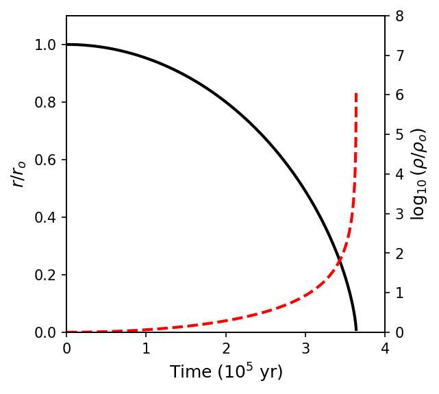
The free-fall time is actually independent of the initial radius of the sphere. AS long as the original density of the spherical molecular cloud was uniform, all parts of the cloud will take the same amount of time to collapse and the density will increase at the same rate everywhere. This behavior is known as homologous collapse. However, if the cloud is somewhat centrally condensed when the collapse begins, the free-fall time will be shorter for material near the center compared to material farther out (i.e., \(t_{\rm ff} \propto 1/\sqrt{\rho_o}\)). As the collapse progresses, the density will increase more rapidly near the center than in the other regions and in this case, the collapse is known as inside-out collapse.
Exercise 8.4
For a dense core of a giant molecular cloud, what is the time required for collapse?
From the example in the Jeans Criterion, we have the initial density \(\rho_o\) and we can find the free-fall timescale by
Equation 20 is transcendental and cannot be solved explicitly. But, numerical root finding techniques can be used. The collapse is slow initially and accelerates as \(t_{\rm ff}\) is approached. At the same time, the density increases most rapidly during the final stages of collapse.
from scipy.constants import G
import numpy as np

def freefall_time(n):
    #n = number density in m^{-3}
    rho_o = n*(2*m_H) #two because its molecular hydrogen H_2
    return np.sqrt(3*np.pi/(32*G*rho_o))/3600./24./365.25 # covert s --> yr

m_H = 1.6735575e-27 #mass of atomic hydrogen in kg
n_H = 1e10 #number density of molecular hydrogen from Jeans mass example

print("The free-fall timescale is %1.2e yr." % freefall_time(n_H))
The free-fall timescale is 3.64e+05 yr.
from scipy.constants import G
from scipy.optimize import root_scalar
import numpy as np
import matplotlib.pyplot as plt

def cloud_collapse(y,t):
    return y + 0.5*np.sin(2*y) - chi*t
m_H = 1.6735575e-27 #mass of atomic hydrogen in kg
n_H = 1e10 #number density of molecular hydrogen from Jeans mass example
rho_o = n_H*(2*m_H)
chi = np.sqrt(8.*np.pi*G*rho_o/3.)*3600.*24.*365.25 #convert s--> yr
h = 100
t_final = 4e5
times = np.arange(0,t_final+h,h)
theta = -np.ones(len(times))

for i in range(0,len(times)):
    try:
        sol = root_scalar(cloud_collapse,x0=0.,bracket=[-1.5,1.5],args=(times[i]),method='bisect')
    except ValueError as VE:
        break
    theta[i] = np.cos(sol.root)**2
t_cut = np.where(theta>0)[0]
times = times[t_cut]
theta = theta[t_cut]

rho = np.log10(1./theta**3)

fs = 'large'
fig = plt.figure(figsize=(4,4),dpi=150)
ax = fig.add_subplot(111)
ax_r = ax.twinx()

ax.plot(times/1e5,theta,'k-',lw=2)
ax_r.plot(times/1e5,rho,'r--',lw=2)

ax.set_ylim(0,1.1)
ax.set_xlim(0,4)
ax_r.set_ylim(0,8)

ax_r.set_ylabel("$\\log_{10}(\\rho/\\rho_o$)",fontsize=fs)

ax.set_xlabel("Time ($10^5$ yr)",fontsize = fs)
ax.set_ylabel("$r/r_o$",fontsize=fs);
8.2.3. The Fragmentation of Collapsing Clouds#
The masses of large molecular clouds could exceed the Jeans limit, which seems to imply that stars can form with very large masses (possibly up to the initial mass of the cloud). However, observations show that this does not happen. It appears that stars frequently tend to form in groups, ranging from binary star systems to clusters that contain hundreds of thousands of members. Some clouds break into segments through a process called fragmentation.
An important consequence of the collapse is that the density of the cloud increases by many orders of magnitude during free-fall. Since the temperature \(T\) remains nearly constant throughout the collapse, it appears that the Jeans mass must decrease. After the collapse begins, any initial inhomogeneities in density will cause individual sections of the cloud to satisfy the Jeans mass limit independently and begin to collapse locally. This cascading collapse could lead to the formation of smaller objects. However, it is likely that only about 1% of the cloud actually forms stars.
What stops the fragmentation process? The answer to this question lies in our implicit assumption that the collapse is isothermal, which in turn implies that the only that changes in the Jeans mass is the density. Clearly this cannot be the case since stars have temperatures much larger than \(10-100\,{\rm K}\). The other extreme is an adiabatic collapse, where the temperature must rise. The real situation lies somewhere between these two limits.
For an adiabatic process the gas pressure is related to its density by \(\gamma\) (the ratio of specific heats). An adiabatic relation between density and temperature can be obtained (using the ideal gas law),
where \(K^{\prime\prime}\) is a constant. Substituting into the equation for the Jeans mass (Eq. (8.10)), we find that
describes how the Jeans mass depends on density. For atomic hydrogen (\(\gamma = 5/3\)), the dependence simplifies to \(M_J \propto \sqrt{\rho}\). The Jeans mass increases with density for a perfectly adiabatic collapse of a cloud. This behavior means the collapse results in a minimum fragment mass that can be produced.
We can make a crude estimate of the lower mass limit of the fragments using the virial theorem. The energy released is roughly,
for a spherical cloud just satisfying the Jeans criterion at some time during the collapse. The luminosity due to gravity is given by
If the cloud were optically thick and in thermodynamic equilibrium, the energy would be emitted as blackbody radiation. During collapse the process is less efficient than for an ideal blackbody and thus we introduce an efficiency factor \(e\) (\(0<e<1\)) that augments the Stefan-Boltzmann equation as
Equating the two expressions (free-fall and blackbody radiation) and solving in terms of the Jeans mass produces
Using the initial cloud radius at a constant density (Eq. (8.9)), and using Eq. (8.10) to write the density in terms of the Jeans mass, we can determine the minimum obtainable Jeans mass:
which depends on the temperature \(T\) (in K), mean molecular weight \(\mu\), and the efficiency factor \(e\). If we take \(\mu \sim 1\), \(e\sim 0.1\), and \(T \sim 1000\,{\rm K}\) to be representative when adiabatic effects become significant, then \(M_J \sim 0.5 M_\odot\). Fragmentation ceases when the segments of the original cloud begin to reach the range of solar mass objects. The estimate is relatively insensitive to other reasonable choices, where if \(e\sim 1\), then \(M_J \sim 0.2 M_\odot\).
8.2.4. Additional Physical Processes in Protostellar Star Formation#
We have freely used the Jeans criterion during each point in the collapse of the cloud to discuss the process of fragmentation. This cannot be correct because our estimate of the Jeans criterions was based on a perturbation to a static cloud (i.e., the initial velocity of the cloud’s outer layers was ignored). The details of radiation transport was also neglected, as well as the vaporization of the dust grains, dissociation of molecules and ionization of the atoms. It is worth noting that the previous analysis produced a result that is reasonable. More sophisticated estimates of the process of fragmentation place the limit at about 0.01 \(M_\odot\), or \(\sim 10 M_{Jup}\).
Other important processes in the collapse process are the effects of rotation (angular momentum), the deviation from spherical symmetry, turbulent motions of the gas, and the presence of magnetic fields. The angular momentum present in the original cloud can result in a disk that leads to the formation of planets.
Careful investigations show that magnetic fields play a crucial role and are likely to control the onset of collapse. From the discussion of the free-fall timescale, the collapse of a dense core should occur after \(10^5\) yr and would imply that as soon as a dense core forms, then it begins producing stars. As a result, the occurrence of dense cores should be quite rare (i.e., we should be privileged to view an event that is so fleeting); however, many dense cores are observable throughout our Galaxy.
Zeeman measurements of various molecular clouds indicate the presence of magnetic fields with strengths from \(1-100\,{\rm nT}\). If the magnetic field of cloud is “frozen-in” and the cloud is compressed, then the magnetic field strength will increase. An increased field strength leads to an increase in the magnetic pressure (as seen in the Sun’s outer atmosphere) and resistance to the compression. The magnetic pressure could be strong enough to prevent the collapse as long as the magnetic field does not decay.
Note
The term “frozen-in” refers to Alfvén’s theorem, which states that “in a fluid with infinite electric conductivity, the magnetic field is frozen into the fluid and has to move along with it.”
The virial theorem was invoked during the derivation of the Jean’s criterion as a balance between the gravitational potential energy and the cloud’s internal (thermal) kinetic energy. The magnetic field energy was ignored, where including the effects of the magnetic field produces a critical mass of
where \(c_B = 380\,{\rm N^{1/2}/m/T}\) for a magnetic field permeating a spherical, uniform cloud. If the magnetic field strength \(B\) is expressed in \({\rm nT}\) and the cloud radius \(R\) in units of \({\rm pc}\), then \(M_B\) can be written as
If the mass of the cloud \(M_c\) is less than \(M_B\), the cloud is said to be magnetically subcritical and stable against collapse. Otherwise, the cloud is magnetically supercritical and the force due to gravity will overwhelm the ability of the magnetic field to resist collapse.
Exercise 8.5
What is the critical mass if the dense core has a magnetic field strength of \(100\,{\rm nT}\) and a radius of \(0.1\,{\rm pc}\)?
The critical mass after including the magnetic field can be calculated as,
implying that a dense core of \(10\,M_\odot\) would be stable against collapse \((M_c < M_B)\). However, if the magnetic field was weaker \((B=1\,{\rm nT})\), then \(M_B \simeq 0.7\,M_\odot\) and collapse would occur.
8.2.5. Ambipolar Diffusion#
Another possibility for triggering the collapse of a dense core is through change of state. If a core that was originally subcritical became supercritical , then collapse could ensue. This could have in a couple of ways:
A group of subcritical clouds could combine to form a supercritical cloud, or
the magnetic field could be rearranged so that the field strength is lessened in a portion of the cloud.
It appears that both processes may occur, although the latter process appears to dominate.
Only charge particles (e.g., electrons, protons, or ions) are tied to magnetic field lines and given that dense molecular cores are dominated by neutral particles, how can magnetic fields have any substantial effect on the collapse? As neutrals try to drift across magnetic field lines, they collide with the “frozen-in” ions and the motions of the neutrals are slowed. If there is a net defined motion of the neutrals due to gravitational forces, then they will still tend to migrate slowly in that direction. This slow migration process is called ambipolar diffusion.
To determine the relative impact of ambipolar diffusion, we need to estimate the characteristic timescale. If we know the drift velocity of the neutrals and the distance across the molecular cloud, then it can be shown that
Exercise 8.6
What is the timescale for ambipolar diffusion within a dense core of a GMC, if \(B = 1\,{\rm nT}\) and \(R = 0.1\,{\rm pc}\)?
The characteristic number density for molecular hydrogen in a dense core is \(n_{\rm H_2} = 10^{10}\,{\rm m^{-3}}\). The timescale for ambipolar diffusion (AD) is then determined as
This is ~\(1000\times\) longer than the free-fall timescale determined for homologous collapse. Clearly the ambipolar diffusion process can control the evolution of a dense core for a long time before free-fall collapse begins.
8.2.6. Numerical Simulations of Protostellar Evolution#
To investigate the nature of gravitational collapse in detail, we must solve the magnetohydrodynamics (MHD) equations numerically. Although computing power has greatly increased, numerical models also make some simplifying assumptions to lessen the computational load and complexity of the output. However, important aspects of the collapse still arise from the numerical solutions.
Consider a spherical cloud of approximately \(1\,M_\odot\) and solar compositions that is supercritical. Initially, the early stages of free-fall collapse are nearly isothermal because the absorption by the dust is relatively inefficient (i.e., photons have a significant mean free path). An initial slight increase in density toward the center of the cloud produces a free-fall time that is shorter near the center and an inside-out collapse can begin. When the density near the center reaches approximately \(10^{-10}\,{\rm kg/m^3}\) (or \(n \sim \times 10^{16}\,{\rm m^{-3}}\)), the region becomes optically thick and the collapse becomes more adiabatic (i.e., heat becomes trapped). The opacity at this point is primarily due to the dust. After the cloud becomes more adiabatic, the gas pressure increases and slows the rate of collapse near the core. The central region (radius of ~\(5\,{AU}\)) is nearly in hydrostatic equilibrium and this central object is then referred to as a protostar.
An observable consequence of the cloud becoming optically thick is that the gravitational potential energy released during the collapse is converted into heat and then radiated away in the IR. By computing the luminosity (i.e., energy release rate) and the cloud radius (for an optical depth \(\tau = 2/3\)), then the effective temperature can be determined via the Stefan-Boltzmann law, \(L = 4\pi R^2 \sigma T^4\), and treating the dust as the photosphere. After which, it becomes possible to plot the location of the simulated cloud on the H-R diagram as a function of time. The curves on the H-R diagram depict the life histories of the simulated clouds are known as evolutionary tracks. As the collapse continues to accelerate, the luminosity of the protostar increases along with its effective temperature.
Above the developing protostellar core, material is still in free-fall. Once that material meets the nearly hydrostatic core, a shock wave develops and the material is supersonic. At this shock front, the infalling material loses a significant fraction of its kinetic energy in the form of heat and produces much of its luminosity. When the temperature reaches ~1000 K, the dust begins to vaporize and the opacity drops. This means the radius corresponding to an optical depth \(\tau = 2/3\) is reduced. Since the luminosity remains high, a corresponding increase in the effective temperature must occur.
The hydrostatic core slowly increases as more overlying material continues to fall onto it. Eventually, the temperatures becomes large enough to cause the molecular hydrogen to dissociate into atomic hydrogen. This process absorbs energy that would otherwise provide a pressure gradient to maintain hydrostatic equilibrium. The core becomes dynamically unstable and a second collapse begins. After the core radius decreases to ~\(1.3\,R_\odot\), hydrostatic equilibrium is re-established. The core mass is still accreting gas, where the final mass will be larger.

Fig. 8.8 Theoretical evolutionary tracks of the gravitational collapse of 0.05, 0.1, 0.5, 1, 2, and 10 \(M_\odot\) clouds through the protostar phase (solid lines). The dashed lines show the times since collapse began. (Carroll & Ostlie (2007))#
After the core collapse, a second shock front is established that continues to heat the infalling material. The main accretion phase when the temperature can increase by several orders of magnitude, while the luminosity remains roughly flat. In this period, the deep interior of the protostar increases enough to start deuterium burning and produces up to 60% of the luminosity of a \(1\,M_\odot\) protostar. The deuterium burning reaction has a fairly large cross section \(\sigma(E)\) at low temperatures and is favored over the PP I chain. Eventually the luminosity must decrease due to a limited amount of initial resources from the original cloud. After the deuterium is exhausted, the evolutionary track bends downward and the effective temperature decreases slightly. The evolution has reached a quasi-static pre-main-sequence phase.
8.3. Pre-Main-Sequence Evolution#
8.3.1. The Hayashi Track#
With the steadily increasing temperature fo the protostar, the opacity of the outer layers becomes dominated with \({\rm H^-}\) ions. The large opacity contributes to starting convection within the contracting protostar. In some cases, the convection zone extends all the way to the center of the star. Chushiro Hayashi demonstrated that a deep convective envelope limits the quasi-static evolutionary path of the protostar to a nearly vertical line in the H-R diagram. As the protostar collapse slows, its luminosity decreases while its effective temperature increases slightly and is known as the Hayashi track (i.e. a downward turn at the end of the evolutionary tracks).
The Hayashi track represents a boundary between “allowed” and “forbidden” hydrostatic stellar models. To the right of the Hayashi track, there is no mechanism to efficiently transport the luminosity out of the star at those low effective temperatures; hence no stable stars exist there. To the left of the Hayashi track, convection and/or radiation is responsible for the energy transport.
8.3.2. Classical Calculations of Pre-Main-Sequence Evolution#
Early models of the final states of collapse neglected the effects of rotation, magnetic fields, and mass loss. Our understanding of the physical processes involved in stellar structure and evolution has improved, which now include nuclear reaction rates, new opacities, mass loss & accretion, and the effects of rotation.
Consider the pre-main-sequence evolution of a 1 \(M_\odot\) star, beginning on the Hayashi track. With the high \({\rm H^-}\) opacity near the surface, the star is completely convective for the first 1 Myr, where deuterium burning also occurs during this early period of the collapse. Since deuterium is not very abundant, the nuclear reactions have little effect on the overall collapse, where they simply slow the collapse rate slightly.
As the central temperature continues to rise, the levels of ionization increase but the opacity decreases.
As the radiative core develops, more of the star’s mass is encompassed by the core.
Following the descent along the Hayashi track, the luminosity reaches a minimum and the radiative core allows energy to escape into the convective envelope more readily.
This causes the luminosity to increase again and the effective temperature increases since the star is still shrinking.
After the luminosity begins to increase, the temperature near the center has become high enough for nuclear reactions to begin, although not yet at their equilibrium rates. The first two steps of the PP I chain and the CNO reactions dominate the nuclear energy production. Over time, these reactions provide an increasingly larger fraction of the luminosity, while the energy due to the gravitational collapse begins to wane.

Fig. 8.9 Classical pre-main-sequence evolutionary tracks computed for stars of various masses with the composition \(X = 0.68\), \(Y = 0.30\), and \(Z = 0.02\). The direction of evolution on each track is generally from low effective temperature to high effective temperature (right to left). The mass of each model is indicated beside its evolutionary track. The square on each track indicates the onset of deuterium burning in these calculations. The long-dash line represents the point on each track where convection in the envelope stops and the envelope becomes purely radiative. The short-dash line marks the onset of convection in the core of the star. Contraction times for each track are given in Table 8.1. (Carroll & Ostlie (2007))#
Initial Mass (\(M_\odot\)) |
Contraction Time (Myr) |
|---|---|
60 |
0.0282 |
25 |
0.0708 |
15 |
0.117 |
9 |
0.288 |
5 |
1.15 |
3 |
7.24 |
2 |
23.4 |
1.5 |
35.4 |
1 |
38.9 |
0.8 |
68.4 |
The CNO reactions have a high temperature dependence and a temperature gradient is established in the core so that some convection begins to develop there. At the local maximum in the luminosity on the H-R diagram (near the end of the track), the nuclear energy production rate is so great that the central core is forced to expand (i.e., \(\epsilon = \epsilon_{nuclear} + \epsilon_{\rm gravity}\)). The expansion causes the total luminosity and temperature to decrease at the surface.
When the carbon-12 is exhausted (for the CNO cycle), the core completes its readjustment to nuclear burning, where the remainder of the PP I chain becomes important. With the establishment of a stable energy source, the gravitational energy term becomes insignificant and the star finally settles onto the main sequence. For stars that are less massive than our Sun, the evolution is somewhat different. These stars never get hot enough in their centers to burn carbon-12 efficiently.
If the protostar mass is \(\lesssim 0.072\,M_\odot\), the core never gets hot enough to generate sufficient energy by nuclear reactions to stabilize the star against gravitational collapse. The stable hydrogen-burning main sequence is never obtained, which explains the lower end of the main sequence. For low mass stars, the temperatures remain cool and opacity stays high such that a radiative core never develops and thus remain fully convective all the way to the main sequence.
8.3.3. The Formation of Brown Dwarfs#
Below about \(0.072\,M_\odot\), some nuclear burning will still occur but not at the rate necessary to form a main-sequence star. Above ~0.06 \(M_\odot\), the core temperature of the star is great enough to burn lithium and above about 0.013 \(M_\odot\) (roughly \(13\,M_{Jup}\)) deuterium burning occurs. The objects between \(0.013-0.072\,M_\odot\) are known as brown dwarfs and have spectral types L and T. The first confirmed discovery of a brown dwarf (Gliese 229B) was announced in 1995. Hundreds of brown dwarfs have been detected in near-IR all-sky surveys, such as 2MASS or SDSS.
8.3.4. Massive Star Formation#
For massive stars, the central temperature quickly becomes high enough to burn carbon-12 and convert hydrogen into helium-3. This means that these stars leave the Hayashi track at higher luminosities and evolve nearly horizontally across the H-R diagram. The full CNO cycle becomes the dominant mechanism for hydrogen burning in these main-sequence stars. The core remains convective even after the main sequence is reached.
8.3.5. Possible Modifications to the Classical Models#
The general pre-main-sequence evolutionary track calculations contain numerous approximations and it is likely that rotation plays an important role, among other factors. These classical models also assume initial structures that are very large. Given that dense cores have dimensions of ~\(0.1\,{\rm pc}\), the initial radii of clouds undergoing protostellar collapse must be much smaller than traditionally assumed. Also, the assumption of pressure-free protostellar collapse may also be incorrect, where more realistic calculations probably require an initial contraction that is quasi-static.
To complicate matters, the more massive stars also interact with infalling material, where a feedback loop may develop that limits the mass accretion via a classical process. Theoretical evolutionary sequences beginning with smaller initial radii lead to a birth line where protostars become visible, which places an upper limit on the observed luminosities of protostars.
Stars with masses greater than 10 \(M_\odot\), may form by a different process, which could be due to limiting feedback mechanisms, such as the high luminosity of ionizing radiation associated with high effective temperatures. Instead of the collapse of single protostellar clouds, the more massive stars may form through mergers of smaller stars in dense protostellar environments (a similar mechanism is proposed for the growth of supermassive black holes, SMBHs). The ionizing radiation problem could be moderated by an accretion disk that feeds the growing massive star through its infalling gas and dust.
8.3.6. The Zero-Age Main Sequence (ZAMS)#
The zero-age main sequence (ZAMS) is known as a diagonal line in the H-R diagram that indicates when stars of various masses reach the main sequence and begin equilibrium hydrogen burning. The amount of time required for stars to collapse onto the ZAMS is inversely related to mas, where a star a little less massive than the Sun \((0.8\,M_\odot)\) takes over 68 Myr to reach the ZAMS and a much more massive star \((60\,M_\odot)\) takes only 28,000 years. This inverse relationship may also signal a problem with classical pre-main-sequence evolutionary models. If the most massive stars form first in clusters, then the intense radiation that they produce would likely disperse the clouds before their low-mass siblings would ever have a chance to develop.
8.3.7. The Initial Mass Function (IMF)#
From observational studies, it appears that more low-mass stars (than high-mass stars) from when an interstellar cloud fragments. The number of stars that form per mass interval per unit volume is strongly mass-dependent, where this functional dependence is known as the initial mass function (IMF). A particular IMF depends on a variety of factors, including the local environment in which a cluster of stars forms. One observational bias arises from the very different evolution rates for star in different mass ranges (i.e., the more massive stars have shorter lifetimes) and thus, it is not surprising that massive stars are extremely rare compared to low-mass stars. Observations also suggest that the curve below \(0.1\,M_\odot\) (or \(\log_{10}\,m = -1\)) may be fairly flat indicating a large number of low-mass stars and brown dwarfs.

Fig. 8.10 Figure 10: The initial mass function, \(\xi\), shows the number of stars per unit area of the Milky Way’s disk per unit interval of logarithmic mass that is produced in different mass intervals. The individual points represent observational data and the solid line is a theoretical estimate. Masses are in solar units. (Carroll & Ostlie (2007))#
8.3.8. \({\rm H\,II}\) Regions#
Hot, massive stars (O and B spectral types) are shrouded in a cloak of gas and dust when they reach the ZAMS. The bulk of their radiation is emitted in the UV, which can ionize the ground-state hydrogen gas \(({\rm H\,I})\) in the ISM to produce \({\rm H\,II}\) regions. The \({\rm H\,II}\) regions are in equilibrium if they have equal rates of ionization and recombination. During recombination, the electron cascades downward and produces a number of lower-energy photons (many will be in the visible). The dominant visible wavelength comes from the \(n=3\) to \(n=2\) transition, or the \({\rm H\alpha}\) line of the Balmer series. Therefore, \({\rm H\,II}\) regions appear to fluoresce in red light.

Fig. 8.11 The \({\rm H\,II}\) region in Orion A is associated with a young OB association, the Trapezium cluster, and a giant molecular cloud. The Orion complex is 450 pc away. (Carroll & Ostlie (2007))#
Emission nebulae are considered to be the most beautiful objects in the night sky, where one particularly famous \({\rm H\,II}\) region is the Orion Nebula (M42). The Orion A complex contains M42, a giant molecular cloud (OMC 1), and a very your star cluster (the Trapezium cluster). The first protostar candidates were discovered in this region as well.
The size of an \({\rm H\,II}\) region can be estimated by considering the equilibrium requirement. Let \(N\) be the number of photons per second produced by a massive O or B star that is producing the ionizing radiation and \(\alpha n_e n_H\) is the number of recombinations per unit volume per second. The latter quantity depends on a quantum-mechanical recombination coefficient that describes the likelihood that a hydrogen atom will recombine given their number densities. At about 8000 K (a temperature characteristic of an \({\rm H\,II}\) region), \(\alpha = 3.1 \times 10^{-19}\,{\rm m^3/s}\). If we assume that the gas is entirely hydrogen and electrically neutral, then the numbers of electrons liberated must equal the number of hydrogen ions (protons), or \(n_e = n_H\). Then the recombination rate can be multiplied by the volume of the \({\rm H\,II}\) region (assumed to be a sphere) and then set equal to the number of ionized photons produced per second. This is expressed as
which solving for the radius produces
and is called the Strömgren radius \(r_S\).
Exercise 8.7
What is the Strömgren radius due to an O6 star in a typical \({\rm H\,II}\) region? (Assume that \(T_e\simeq 45,000\,{\rm K}\) and \(L\simeq 1.3\times10^5\,L_\odot\))
From Wien’s law, the peak wavelength is given as
This is significantly shorter (or higher energy) than the 91.2-nm limit (\({\rm Ly_{\rm limit}}\) from the wavelength of hydrogen) and it can be assumed that most of the photons created by an O6 star are capable of causing ionization. The energy of one 64-nm photon can be calculated giving
Assuming that all of the emitted photons have the same (peak wavelength), then the total number of photons produced per second is just
Lastly, a typical the number density within a GMC is \(n_H \sim 10^8\,{\rm m^{-3}}\), we find
Values of \(r_S\) range from less than 0.1 pc to greater than 100 pc.
from scipy.constants import h,c,Wien,pi,parsec

def Wien_law(T_e):
    #T_e = effective temperature in K
    return Wien/T_e #returns value in m

def photon_energy(lam):
    #lam = wavelength in m
    return h*c/lam #return value in J

def Stromgren_radius(N,n_H):
    #N = total number of photons produced by the star
    #n_H = number density of hydrogen
    return (3*N/(4*pi*alpha*n_H**2))**(1./3.)/parsec #returns the Stromgren radius in pc

L_sun = 3.827e26 #Solar luminosity in W
T_e = 45000 #effective temperature of an O6 star
L_star = 1.3e5*L_sun #luminosity of an O6 star in W
n_H = 1e8 #number density of hydrogen atoms in a GMC
alpha = 3.1e-19 #recombination coefficient for a typical H II region

E_peak = photon_energy(Wien_law(T_e))
N = L_star/E_peak

print("The total number of photons produced per second is approximately %1.2e" % N)

r_S = Stromgren_radius(N,n_H)
print("The Stromgren radius due to an O6 star is %1.2f pc." % r_S)
The total number of photons produced per second is approximately 1.61e+49
The Stromgren radius due to an O6 star is 3.48 pc.
8.3.9. The Effects of Massive Stars on Gas Clouds#
Through the formation of massive protostars, the temperature will begin to rise in the molecular cloud, where the dust will vaporize and molecules will dissociated before the star reaches the main sequence. After reaching the main sequence, the surrounding gas will ionize, resulting tin the creation of a \({\rm H\,II}\) region inside of a \({\rm H\,I}\) region. Due to the star’s high luminosity, radiation pressure will begin to drive significant mass loss that can disperse the remainder of the cloud. If several O and B stars form at the same time, then star formation can be halted around other protostars as they are starved for resources. If the cloud was only marginally bound, the mass loss will result in the newly formed stars drifting apart from the initial cluster. Some famous examples of this occurring are in the Carina Nebula (about 3000 pc from Earth) and in the Eagle Nebula (M16).

Fig. 8.12 A Visible image of a portion of the Carina Nebula (top). The same region observed in IR (bottom). Much less detail is observable because of the obscuration due to dust in the cloud. (Carroll & Ostlie (2007); HST/ESA)#
8.3.9.1. OB Associations#
Groups of stars that are dominated by O and B main-sequence stars are called OB associations, where studies show that they cannot remain gravitationally bound to on another due to their individual kinematic velocities and masses. An example is in the Trapezium cluster in the Orion A complex, which is believed to be less than 10 million years old. It is currently densely populated with stars \((>2000\,{\rm pc^{-3}})\) that are in the range of \(0.5-2.0\,M_\odot\). Radial velocity measurements (in \(^{13}CO\)) show that the gas in the vicinity is very turbulent, where the nearby O and B stars are dispersing the gas and causing the cluster to become unbound.

Fig. 8.13 Figure 13: The giant gas pillars of the Eagle Nebula (M16). The left most pillar is more than 1 pc long from base to top. Ionizing radiation from massive newborn stars off the top edge of the image are causing the gas in the cloud to photoevaporate. [Courtesy of NASA, ESA, STScI, J. Hester and P. Scowen (Arizona State University).]#
8.3.9.2. T Tauri Stars#
There is a low-mass pre-main-sequence object that represents a transition from protostars still shrouded in dust and main-sequence stars, which is called a T Tauri star. These objects are named after the first star of their class located in the constellation Taurus. T Tauri stars are characterized by unusual spectral features and by large irregular luminosity variations (with timescales on the order of days). The masses of T Tauri stars range from \(0.2-2.0\,M_\odot\). Many T Tauri stars also exhibit strong emission from hydrogen (i.e., the Balmer series) \({\rm Ca\,II}\) (H and K), iron, and lithium. The forbidden lines \(({\rm O\,I\,and\,S\,II})\) are also present. The existence of forbidden lines is an indication of extremely low gas densities.
Information can be gleaned from spectra using the shapes of the lines as a function of wavelength. In T Tauri stars, the \({\rm H\alpha}\) line often exhibits a characteristic shape, where an absorption trough (at the short-wavelength edge of the line) is superimposed on a rather broad emission peak. This unique line shape is called a P Cygni profile, which is named after the first star observed to have emission lines with a blueshifted absorption trough. The existing of a P Cygni profile indicates that the star is losing mass significantly. From Kirchhoff’s law, emission lines are produced by a hot, diffuse gas with little intervening material. In this case, the emission source is an expanding shell moving perpendicular to our line of sight. Absorption lines are the result of light passing through a cooler, diffuse gas. the mass loss rates of T Tauri stars average about \(\dot{M}= 10^{-8}\,M_\odot/{\rm yr}\). In some extreme cases, T Tauri stars appear to accrete mass rather than lose it, where the P Cygni profile is inverted (redshifted absorption). Mass accretion rates appear similar to mass loss rates.
8.3.9.3. FU Orionis Stars#
A T Tauri star star can go through a significant increase in its mass accretion rate \((\dot{M} = 10^{-4}\,M_\odot/{\rm yr})\) and luminosity (by four orders of magnitudes or more) that lasts for decades. The firs star to undergo these abrupt changes was FU Orionis, where similar behaving stars are called FU Orionis stars. Instabilities in a circumstellar accretion disk can result in \(\sim 0.01\,M_\odot\) being dumped onto the central star to cause the outburst. The inner disk can outshine the central star by a factor of \(100-1000\), while high-velocity winds \((>300\,{\rm km/s})\) occur.
8.3.9.4. Herbig Ae/Be Stars#
Closely related to the T Tauri stars are Herbig Ae/Be stars, named for George Herbig. These pre-main-sequence A or B stars have strong emission lines (and hence the e designation). Their masses range from \(2-10\,M_\odot\) and tend to be shrouded in some remaining gas and dust.
8.3.9.5. Herbig-Haro Objects#
Mass loss during pre-main-sequence evolution can also occur from jets of gas that are ejected in narrow beams in opposite directions. Herbig-Haro objects (HH objects) were discovered in the early 1950s by George Herbig and Guillermo Haro in the vicinity of the Orion nebula and are associated with the jets produced by young protostars (e.g., T Tauri stars). Jets can excite gas within the ISM, which results in objects with bright emission line spectra. Herbig-Haro objects HH 1 and HH 2 were created by material ejected at speeds of several 100 \({\rm km/s}\) from a star shrouded in a cocoon of dust.

Fig. 8.14 (a) A jet associated with HH 47. The scale at the lower left is 1000 AU. (Courtesy of J. Morse/STScI, and NASA.) (b) The Herbig–Haro objects HH 1 and HH 2 are located just south of the Orion nebula and are moving away from a young protostar hidden inside a dust cloud near the center of the image. [Courtesy of J. Hester (Arizona State University), the WF/PC 2 Investigation Definition Team, and NASA.]#
Continuous emission is also observed in some protostellar (circumstellar) objects and is from the reflection of light from the parent star (e.g., HH 30). The surfaces of a circumstellar disk are illuminated by the central star, which is hidden from view behind the dusty disk. Jets are originating from deep within the accretion disk, possibly from the star. These accretion disks appear responsible for emission lines, mass loss, jets and even some of the luminosity variations. Unfortunately, the details are not fully understood, but early models can be developed.

Fig. 8.15 An early model of a T Tauri star with an accretion disk. The disk powers and collimates jets that expand into the interstellar medium, producing Herbig–Haro objects. (Carroll and Ostlie (2007); Figure adapted from Snell, Loren, and Plambeck, Ap. J. Lett., 239, L17, 1980.)#
8.3.10. Young Stars with Circumstellar Disks#
Observations have revealed that other young stars also possess circumstellar disks of material, where two well-known examples are Vega and \(\beta\) Pictoris. An IR image of \(\beta\) Pic shows its disk, where observations of \(\beta\) Pic in the UV suggest that clumps of material are falling from the disk into the star at a rate of 2-3 per week. There are indications of two substellar objects (planets or brown dwarfs) interacting with a debris disk to form resonance gaps.
8.3.10.1. Proplyds#
he Orion Nebula was observed in 1993 by HST, where the observations used the emission lines of \({\rm H\alpha}\) and the two forbidden lines \(({\rm N\, II\; and\, O\,III})\). Analysis of the data revealed 56 (out of 110 stars) brighter than \(V= 21\) are surrounded by disks of circumstellar dust and gas. Proplyds, or protoplanetary disks associated with young stars are less than 1 Myr old. Based on observations of the ionized material in the proplyds, the disks seem to have masses much greater than \(\sim 4\,M_\oplus\).

Fig. 8.16 Images of the Orion Nebula (M42) obtained by the Hubble Space Telescope. Numerous proplyds are visible in the field of view of the camera. (Courtesy of C. Robert O’Dell/Vanderbilt University, NASA, and ESA.)#
8.3.10.2. Circumstellar Disk Formation#
Disk formation is fairly common during the collapse of protostellar clouds due to the spin-up of the cloud as required by the conservation of angular momentum. As the radius of the protostar decreases does its moment of inertia. In the absence of external torques, the protostar’s angular velocity must increase.
A problem immediately arises when the effect of angular momentum is included in the collapse. Conservation of angular momentum arguments suggest that all main sequence stars should be rotating very rapidly (at rates close to breakup). However, this is generally not seen in observations, where the angular momentum must be transferred away from the collapsing star. One suggestion is that magnetic fields slow the rotation by applying torques (i.e., magnetic braking). Additionally, star-disk or star-planet interactions are likely to play a role in distributing the angular momentum.
8.4. Homework#
Problem 1
In a certain part of the North American Nebula, the amount of interstellar extinction in the visual wavelength band is 1.1 magnitudes, the thickness of the nebula is estimated to be 20 pc, and it is located 700 pc away from Earth. Suppose that a B spectral class main-sequence star is observed in the direction of the nebula and that the absolute visual magnitude of the star is known to be \(M_V = -1.1\). Neglect any other sources of extinction between the observer and the nebula. (a) Find the apparent visual magnitude of the star if it is lying just in front of the nebula.
(b) Find the apparent visual magnitude of the star if it is lying just behind the nebula.
(c) Without taking the existence of the nebula into consideration (based on its apparent magnitude), how far away does the star in part (b) appear to be? What would be the percentage error in determining the distance if the interstellar extinction were neglected?
Problem 2
An \({\rm H\,I}\) cloud produces a 21 cm line with an optical depth at its center of \(\tau_H = 0.5\) (i.e., the line is optically thin). The temperature of the gas is 100 K, the line’s FWHM is \({10\,{\rm km/s}}\), and the average atomic number density of the cloud is \(10^7\,{\rm m^{-3}}\). Find the thickness of the cloud. Express your answer in pc.
Problem 3
In light of the cooling mechanisms discussed for molecular clouds, explain why dense cores are generally cooler than the surrounding giant molecular clouds, and why GMCs are cooler than diffuse molecular clouds.
Problem 4
Show that the Jeans mass can also be written in the form
where the isothermal sound speed \(v_T \equiv \sqrt{kT/(\mu m_H)}\), the pressure \(P_o\) associated with the density \(\rho_o\) and temperature \(T\), and there is a dimensionless constant \(c_J \simeq 5.46\).
Problem 5
Assuming that the free-fall acceleration of the surface of a collapsing cloud remains constant during the entire collapse, derive an expression for the free-fall time. Show that your answer differs from Eq. (8.21) only by a term of order unity.
Problem 6
Assuming a mass loss rate of \(10^{-7}\, M_\odot/{\rm yr}\) and a stellar wind velocity of \(80\,{\rm km/s}\) from a T Tauri star,
(a) estimate the mass density of the wind at a distance of 100 AU from the star, and
(b) compare your answer in (a) with the density of the giant molecular cloud \((\rho_o=3\times 10^{-17}\,{\rm kg/m^{-3}})\).