2. The Interaction of Matter and Light#
2.1. Spectral Lines#
Some philosophers during the Renaissance considered strict limits to human knowledge, while other natural philosophers used experimentation to probe reality. In 1800, William Wollaston showed that a number of dark spectral lines were present within the a rainbow-like spectrum using sunlight. By 1814, Joseph von Fraunhofer cataloged 475 of the dark lines (i.e., Fraunhofer lines) in the solar spectrum. Fraunhofer determined that the wavelength of one prominent dark line in the Sun’s spectrum corresponds to the yellow light emitted by salt in a flame. The new science of spectroscopy was born with the discovery of the sodium line.

Fig. 2.1 Solar spectrum with Fraunhofer lines as it appears visually. Image Credit: Wikipedia:Fraunhofer lines.#
Wavelength (nm) |
Name |
Atom |
Equivalent Width (nm) |
|---|---|---|---|
385.992 |
\(\rm Fe\ I\) |
0.155 |
|
388.905 |
\(\rm H_8\) |
0.235 |
|
393.905 |
\(\rm K\) |
\(\rm Ca\ II\) |
2.025 |
396.849 |
\(\rm H\) |
\(\rm Ca\ II\) |
1.547 |
404.582 |
\(\rm Fe\ I\) |
0.117 |
|
410.175 |
\({\rm h,\ H}\delta\) |
\(\rm H\ I\) |
0.313 |
422.674 |
\(\rm g\) |
\(\rm Ca\ I\) |
0.148 |
434.048 |
\({\rm G}^\prime,\ {\rm H}\gamma\) |
\(\rm H\ I\) |
0.286 |
438.356 |
\({\rm d}\) |
\(\rm Fe\ I\) |
0.101 |
486.134 |
\({\rm F},\ {\rm H}\beta\) |
\(\rm H\ I\) |
0.286 |
516.733 |
\(b_4\) |
\(\rm Mg\ I\) |
0.065 |
517.270 |
\(b_2\) |
\(\rm Mg\ I\) |
0.126 |
518.362 |
\(b_1\) |
\(\rm Mg\ I\) |
0.158 |
588.997 |
\({\rm D_2}\) |
\(\rm Na\ I\) |
0.075 |
589.594 |
\({\rm D_1}\) |
\(\rm Na\ I\) |
0.056 |
656.281 |
\({\rm C},\ {\rm H}\alpha\) |
\(\rm H\ I\) |
0.402 |
2.1.1. Kirchoff’s Laws#
The foundations of spectroscopy (and modern chemistry) were established in the 1800s with Robert Bunsen and Gustav Kirchhoff. Bunsen’s burner produced a colorless flame that was ideal for studying the colors produced by burning a range of substances. Bunsen and Kirchoff designed a spectroscope that passed the light of a flame spectrum through a prism. They determined that the wavelengths of light absorbed and emitted by an element fit together like a lock and key. Kirchoff determined that 70 of the Fraunhofer lines were due to iron vapor. In 1860, Kirchoff and Bunsen developed the idea that every element produces its own pattern of spectral lines and thus the elements had “fingerprints”. Kirchoff summarized the production of spectral lines in three laws (i.e., Kirchoff’s Laws):
A hot, dense gas or hot solid object produces a continuous spectrum with no dark spectral lines.
A hot diffuse gas produces bright spectral lines (emission lines).
A cool, diffuse gas in front of a source of a continuous spectrum produces dark spectral lines (absorption lines) in the continuous spectrum.
2.1.2. Applications of Stellar Spectral Data#
Using the development of spectral fingerprints, a new element helium was discovered spectroscopically in the Sun (in 1868) and found on Earth in 1895. Another line of investigation was measuring the Doppler shifts of the spectral lines. For most cases at the time, the low-speed approximation (\(v_r \ll c\)) was adequate to determine the radial velocities \(v_r\) by the following equation,
By 1887, the radial velocities of Sirius, Procyon, Rigel, and Arcturus were measured with and accuracy of a few km/s. The rest wavelength \(\lambda_{\rm rest}\) for the hydrogen spectral line (\({\rm H}_\alpha\)) is 656.281 nm (in air). Given the simplicity of hydrogen and its spectral lines, they are commonly used to measure the radial velocities of stars.
Exercise 2.1
What is the radial velocity of the star Vega, if its \({\rm H}_\alpha\) line is observed at 656.21 nm from a ground-based telescope? (There is a typographical error in the textbook.)
Applying the low-speed approximation for the radial velocity, we get:
import numpy as np
from scipy.constants import c

def calc_radial_vel(l_obs,l_rest):
    #l_obs = the observered wavelength
    #l_rest = the rest wavelength measured in a lab
    #the units of l_obs must equal l_rest
    rad_vel = (l_obs-l_rest)/l_rest
    return rad_vel*c

Ha_obs = 656.251 #Vega H-alpha in nm
Ha_rest = 656.281 #rest H-alpha in nm
Vega_RV = calc_radial_vel(Ha_obs,Ha_rest)/1000 #convert from m/s to km/s
print("The radial velocity of Vega is %2.3f km/s." % np.round(Vega_RV,3))
The radial velocity of Vega is -13.704 km/s.
The negative sign for the radial velocity indicates that Vega is approaching the Sun (i.e., moving towards us). Some stars also have a measured proper motion \(\mu\) that is perpendicular to the line-of-sight. Combining the proper motion with a known distance \(r\), the transverse velocity \(v_\theta\) can be determined (\(v_\theta = r\mu\)).
Exercise 2.2
Vega’s proper motion is \(\mu = 0.34972^{\prime \prime}/{\rm yr}\) and its distance is 7.68 \({\rm pc}\) away (Van Leeuwen 2007). What is its tranverse velocity? What is its velocity through space?
The velocity through space is determined by combining the radial velocity with the proper motion. From the previous problem, we know that Vega’s radial velocity \(v_r = -13.704\ {\rm km/s}\). To get the tranverse velocity, we need to convert the proper motion (in \(^{\prime \prime}\)/yr) and the distance to Vega (in \(\rm pc\)) into SI units. Converting these quanties gives,
The tranverse velocity can be calculated as
Finally, the velocity through space can be determined through the hypotenuse of two vector components,
#get constants from scipy; https://docs.scipy.org/doc/scipy/reference/constants.html
from scipy.constants import astronomical_unit, year

def mu2SI(mu):
    #mu = proper motion (in arcseconds/year)
    #mu * (arcseconds in a radian)/(seconds in a year)
    mu *= (as2rad/year)
    return mu
def PC2km(r):
    #r = distance in pc
    r2AU = r/as2rad #pc converted to AU
    r2km = r2AU*AU #convert to km
    return r2km

AU = astronomical_unit/1000. #(in km) Astronomical Unit
as2rad = (1./3600.)*(np.pi/180.)
mu = mu2SI(0.34972)
r = PC2km(7.68)
v_theta = r*mu
print("The transverse velocity of Vega is %2.1f km/s." % np.round(v_theta,1))
v_Vega = np.sqrt(v_theta**2+Vega_RV**2)
print("Vega's velocity through space is %2.1f km/s" % (v_Vega))
The transverse velocity of Vega is 12.7 km/s.
Vega's velocity through space is 18.7 km/s
The average speed of stars in the solar neighborhood is about 25 km/s, where the measurement of a star’s radial velocity is also complicated by the motion of the Earth (29.8 km/s) around the Sun. Astronomers correct for this motion by subtracting the component of Earth’s orbital velocity along the line-of-sight from the star’s measured radial velocity.
2.1.3. Spectrographs#
Modern methods can measure radial velocities with an accuracy of \(\sim 1\) m/s (Dumusque et al. 2021). Astronomers use spectrographs to measure the radial velocity of exoplanets, stars, and galaxies. Modern spectrographs collimate the incoming starlight onto a mirror and split into the constituent colors using a diffraction grating, or a piece of glass with narrow, closely spaced lines; a transmission grating allows the light to pass through while a reflection grating reflects the light. The grating acts like a series of neighboring double slits (see Chapter 3). Different wavelengths have their maxima occurring at different angles \(\theta\) by
where \(d\) is the slit spacing of the grating, \(n\) is the order of the spectrum, and \(\theta\) is measured relative the line perpendicular to the grating. The smallest measurable difference in wavelength \(\Delta \lambda\) depends on the order \(n\) and the total number of lines \(N\) through
where \(\lambda\) is either of the closely spaced wavelengths. The ratio \(\lambda/\Delta \lambda\) is one way to express the resolving power of the grating.

Fig. 2.2 Schematic of a spectrograph. Image Credit: Scientific American.#
2.2. Photons#
A complementary description of light (in contrast to waves) uses bundles of energy called photons. The energy is described in terms of Planck’s constant h and is recognized as a fundamental constant of nature like the speed of light c. This description of matter and energy is known as quantum mechanics, which uses Planck’s discovery of energy quantization. The first step forward was made by Einstein, who demonstrated the implications of Planck’s quantum bundles of energy.
2.2.1. The Photoelectric Effect#
The photoelectric effect describes the light energy necessary to eject electrons from a metal surface. The electrons with the highest kinetic energy \(K_{max}\) originate from the surface of the metal and surprisingly, \(K_{max}\) does not depend on the light intensity. A higher intensity of light increases the number of electrons ejected, but not their maximum kinetic energy. The value of \(K_{max}\) varies with the frequency of the light and each metal has a characteristic cutoff frequency \(\nu_c\) and wavelength \((\lambda_c = c/\nu_c\)).
Einstein’s solution describes the light striking the metal surface as a stream of massless particles (i.e., photons). The energy of a single photon of frequency \(\nu\) and wavelength \(\lambda\) is just Planck’s quantum of energy
Exercise 2.3
What is the energy of a single blue photon of wavelength \(\lambda = 450\) nm?
We can find the energy of a single photon in units of \({\rm eV}\) or \({\rm J}\). It is more common to use units of \({\rm eV}\) because there is a well defined value for the product of Planck’s constant \(h\) with the speed of light \(c\), or \(hc = 1240\ {\rm eV\cdot nm}\). As a result, we find the energy as,
from scipy.constants import h

def energy_photon(l,units):
    #l = lambda; wavelength in nm
    if units=='eV':
        hc = 1240 #eV*nm
    else:
        #h = 6.62607004e-34 #(m^2*kg/s) Planck's constant
        hc = h*c*1000/1e-9
    return (hc/l)

E_blue_eV = energy_photon(450,'eV')
E_blue_J = energy_photon(450,'J')
print("The energy of a single blue photon (450 nm) is %1.2f eV or %1.2e J" % (np.round(E_blue_eV,2),E_blue_J))
The energy of a single blue photon (450 nm) is 2.76 eV or 4.41e-16 J
Einstein deduced that when a photon strikes the metal surface, its energy may be absorbed by a single electron. The photon supplies the energy required to free the electron from the metal (i.e., overcome the binding energy). The work function \(\phi\) defines the minimum binding energy of electrons in a metal and the maximum kinetic energy of the ejected electrons is
where the cutoff frequency and wavelength are \(\nu_c = \phi/h\) and \(\lambda_c = hc/\phi\), respectively. Albert Einstein was awarded the 1921 Nobel Prize for “his services to theoretical physics, and especially for his discovery of the law of the photoelectric effect”. Astronomers take advantage of the photoelectric effect through detectors that count photons by the work they do on a metal (e.g., charge-coupled devices or CCDs).
2.2.2. The Compton Effect#
Another test of light’s particle-like nature was performed by Arthur Compton. He measured the change in the wavelength of X-ray photons as they were scattered by free electrons. Through special relativity, the energy of a photon is related to its momentum \(p\) by
Compton considered the interaction (or “collision”) between a photon and a free electron (initially at rest). The electron is scattered by an angle \(\varphi\), while the photon is scattered by an angle \(\theta\). Due to the energy exchange during the interaction (i.e., electron gains kinetic energy) the photon’s energy is reduced and the wavelength has increased. The change in wavelength is the difference between the final and initial wavelength and can be expressed as
where \(m_e\) is the mass of the electron. The prefactor \(h/m_e c\) is called the Compton wavelength \(\lambda_C\). Compton’s experiment provided evidence that photons carry momentum (although massless) and this is the physical basis for the force exerted by radiation upon matter.
Fig. 2.3 The Compton effect: the scattering of a photon by a free electron. Image Credit: hyperphysics.#
2.3. The Bohr Model of the Atom#
2.3.1. The Structure of the Atom#
With the discovery of the electron (by J.J. Thomson), it showed that the atom is composed of smaller parts usually consisting of electrically neutral bulk matter (equal parts of negative and positive charges). Ernest Rutherford discovered in 1911 that an atom’s positive charge was concentrated in a tiny, massive nucleus using \(\alpha\) particles (now know to be helium nuclei). Rutherford calculated that the radius of the nucleus was 10,000 times smaller than the atomic radius showing that ordinary matter is mostly empty space. Rutherford also coined the term proton to refer to the nucleus of the hydrogen atom and is 1836 times more massive than the electron.
2.3.2. The Wavelength of Hydrogen#
Many natural philosophers (now known as chemists) produced a wealth of experimental data. Fourteen spectral lines of hydrogen had been precisely measured before the 20th century. The spectral lines were described by their wavelengths and categorized using greek letters (\({\rm H}\alpha\), \({\rm H}\beta\), etc.). In 1885 Johann Balmer found (by trial and error) a formula to reproduce the series of wavelengths for hydrogen’s spectral lines (or Balmer lines) given as
where \(n\) is an integer greater than 2 (\(n=3,4,5,\ldots\)) and \(R_H = 1.09677583 \times 10^7 \pm 1.3 \;{\rm m}^{-1}\) is the Rydberg constant) for hydrogen. Equation (2.7) is accurate to a fraction of a percent, where values of \(n\) produce the wavelength for the spectral lines (\({\rm H}\alpha\), \({\rm H}\beta\), \({\rm H}\gamma\), etc. ). Balmer realized that the formula could be generalized (since \(2^2 = 4\)) producing the general form as
with \(m<n\) (both integers). There are only a few spectral lines that lie in the visible range for hydrogen, where the Lyman lines (\(m=1\)) are found in the ultraviolet and the Paschen lines (\(m=3\)) lie entirely in the infrared.
Series Name |
Symbol |
Transition |
Wavelength (nm) |
|---|---|---|---|
Lyman |
\({\rm Ly\alpha}\) |
\(2 \leftrightarrow 1\) |
121.567 |
\({\rm Ly\beta}\) |
\(3 \leftrightarrow 1\) |
102.572 |
|
\({\rm Ly\gamma}\) |
\(4 \leftrightarrow 1\) |
97.254 |
|
\({\rm Ly_{limit}}\) |
\(\infty \leftrightarrow 1\) |
91.18 |
|
Balmer |
\({\rm H\alpha}\) |
\(3 \leftrightarrow 2\) |
656.281 |
\({\rm H\beta}\) |
\(4 \leftrightarrow 2\) |
486.134 |
|
\({\rm H\gamma}\) |
\(5 \leftrightarrow 2\) |
434.048 |
|
\({\rm H\delta}\) |
\(6 \leftrightarrow 2\) |
410.175 |
|
\({\rm H\epsilon}\) |
\(7 \leftrightarrow 2\) |
397.007 |
|
\({\rm H_8}\) |
\(8 \leftrightarrow 2\) |
388.905 |
|
\({\rm H_{limit}}\) |
\(\infty \leftrightarrow 2\) |
364.6 |
|
Paschen |
\({\rm Pa\alpha}\) |
\(4 \leftrightarrow 3\) |
1875.10 |
\({\rm Pa\beta}\) |
\(5 \leftrightarrow 3\) |
1281.81 |
|
\({\rm Pa\gamma}\) |
\(6 \leftrightarrow 3\) |
1093.81 |
|
\({\rm Pa_{limit}}\) |
\(\infty \leftrightarrow 3\) |
820.4 |
Exercise 2.4
What are the first 3 wavelengths for the Balmer, Lyman, and Paschen lines? (Compare to Table 2 in Ch 5 of the textbook)
The first 3 wavelengths of each series can be estimated using the Rydberg equation using integers \(m\) and \(n\). It is also convenient to known the Rydberg constant in nm, where \(R_H = 1.097373156816 \times 10^{-2}\ {\rm nm^{-1}}\). The Rydberg equation is given as
Then, the first term of each series is given as
from scipy.constants import Rydberg
def calculate_lambda_mn(m,n):
    #m,n = integers
    if m < n:
        return (1./R_H)*(m**2*n**2)/(n**2-m**2)
    else:
        print("Please choose appropriate values for m,n (m<n)")
        return 0

R_H = Rydberg*1e-9 #Rydberg constant in nm

Balmer = np.zeros(3)
Lyman = np.zeros(3)
Paschen = np.zeros(3)
wavelength = [Balmer,Lyman,Paschen]
for i in range(1,4):
    Balmer[i-1] = calculate_lambda_mn(2,2+i)
    Lyman[i-1] = calculate_lambda_mn(1,1+i)
    Paschen[i-1] = calculate_lambda_mn(3,3+i)
Series = ["H","Ly","Pa"]
letter = ["$\\alpha$","\$beta$","$\gamma$"]
for i in range(0,3):
    for j in range(0,3):
        print("%s%s is %3.3f nm." % (Series[i],letter[j],wavelength[i][j]))
H$\alpha$ is 656.112 nm.
H\$beta$ is 486.009 nm.
H$\gamma$ is 433.937 nm.
Ly$\alpha$ is 121.502 nm.
Ly\$beta$ is 102.518 nm.
Ly$\gamma$ is 97.202 nm.
Pa$\alpha$ is 1874.607 nm.
Pa\$beta$ is 1281.469 nm.
Pa$\gamma$ is 1093.520 nm.
Although this formula worked for hydrogen, physicists of the day wanted a physical model that could be applied more broadly. The simplest “planet-like” model of an electron orbiting a proton was the most attractive, but Maxwell’s equations predicted a basic instability. A particle in a circular orbit experiences an acceleration, where Maxwell showed that accelerating charges emit electromagnetic radiation. Under this model, the electron would lose energy by emitting light as it spirals down into the nucleus in only \(10^{-8}\) s. Obviously this wasn’t a good description of nature.
2.3.3. Bohr’s Semiclassical Atom#
In 1913, Niels Bohr noted that the dimensions of Planck’s constant are equivalent to angular momentum and perhaps the angular momentum of the orbiting electron was quantized. Bohr hypothesized that orbits with integral multiples of Planck’s constant (i.e., a specific angular momentum), the electron would be stable and would not radiate in spite of its centripetal acceleration.

Fig. 2.4 Bohr atom with an electron revolving around a fixed nucleus. Image Credit: Ümit Kaya; Libretexts.#
To analyze the interactions between a proton and electron, we start with the mathematical description given by Coulomb’s law. The electric force between two charges (\(q_1\) and \(q_2\)) separated by a distance \(r\) has the familiar form
where \(\epsilon_o = 8.854187817\ldots \times 10^{-12}\) F \({\rm m}^{-1}\) is the permittivity of free space and \(\hat{{\bf r}}\) is a unit vector that points from \(q_1\) to \(q_2\). In the hydrogen atom, the electron has a negative charge \(e^-\) and the proton a positive charge \(e^+\). The Coulomb force pulls opposite charges toward on another, which is definitely not a good description of the system. In the case of two masses orbiting each other, we set the gravitational force equal the centripetal force. Thus, it follows that we could try the same procedure for a proton of mass \(m_p\) and an electron of mass \(m_e\). Simplifying further, we can convert the two-body problem to an equivalent one-body problem using the reduced mass
where \(m_p = 1836.15266 m_e\) and the total mass \(M = m_e+m_p\). To evaluate the one-body problem, we use a coordinate system so that the proton is at the origin (i.e., proton-centric). Note: this technique is also used in orbital mechanics where planetary systems are evaluate in heliocentric coordinates. Using the centripetal acceleration and Newton’s second law:
which can be solved for the kinetic energy \(K\):
The electrical potential energy \(U\) of the Bohr atom is:
The total energy \(E = K + U\) of the atom is:
The kinetic energy is a positive quantity, which implies that the total energy is negative and indicates that the electron and proton are bound. To ionize or free the electron, it must receive at least an amount of energy equal to \(|E|\).
Getting back to Bohr’s contribution, he suggested that the angular momentum \(L = \mu vr\) was quantized and could be expressed in terms of Planck’s constant \(h\) distributed over a unit circle as \(\hbar = h/2\pi\). The full condition is
which can be rewritten using the kinetic energy as
Solving the second line of the equation above for the radius \(r\) shows that the specific values are allowed by Bohr’s quantization condition as
where \(a_o = 5.291772083 \times 10^{-11}\) m is known as the Bohr radius. Now that we know the scale of the atom (i.e., appropriate values of \(r\)), the energy in terms of fundamental constants are given as
The principal quantum number \(n\) completely determines the characteristics of the Bohr atom, where \(n\geq 1\).
The spectral lines are produced by electron transitions within the atom (i.e., moving between energy levels). Balmer tried to produce a formula that would predict the wavelength that resulted from a transition from \(n_{high}\rightarrow n_{low}\). Now consider the required energy to move between levels as the energy of a photon \(E_{photon} = hc/\lambda = E_{high} - E_{low}\), which gives
where \(hc = 1240\) eV nm.
Exercise 2.5
What are the first 3 wavelengths in the Balmer lines using this method?
In this method, we can evaluate the wavelengths using \(n_{low} = 2\) and use \(hc/13.60569\ {\rm eV} = 91.13832\ {\rm nm}\) as the prefactor. The resulting expression for the Balmer series is
where \(n\) is an integer representing the higher energy state. The first wavelength is given as
from scipy.constants import physical_constants
R_H = physical_constants['Rydberg constant times hc in eV'][0]

def calculate_lambda_hl(n_h,n_l):
    #n_h = higher state
    #n_l = lower state
    if n_h > n_l:
        return (1240/R_H)*(n_h**2*n_l**2)/(n_h**2-n_l**2)
    else:
        print("Please choose appropriate values for n_h,n_l (n_l<n_h)")
        return 0

for i in range(0,1):
    for j in range(0,3):
        B_lam = calculate_lambda_hl(j+3,2)
        print("%s%s is %3.3f nm." % (Series[i],letter[j],B_lam))
H$\alpha$ is 656.196 nm.
H\$beta$ is 486.071 nm.
H$\gamma$ is 433.992 nm.
The above results and those produced from Balmer’s formula are for light traveling in a vacuum. The empirical measurements are made in air, where the speed of light is slightly slower by a factor of 0.999703 and \(\lambda_{\rm air} = 0.999703 \lambda_{\rm vacuum}\). Solving for the \({\rm H}\alpha\) line in air yields \(\lambda_{\rm air} = 656.276\) nm, which differs from the quoted value by 0.0008%. The remainder of the discrepancy is due to environmental factors (e.g., temperature, pressure, and humidity) that affect the index of refraction for air.
This discussion has focused on electrons that transition from a higher (large \(n\)) to lower (small \(n\)) energy state. But, the reverse process can occur, where a photon is absorbed by the atom thereby exciting an electron from a lower to a higher energy state. The former process produces spectral emission where the latter produces absorption and Eqn. 15 is used for both processes. Kirchoff’s laws now had a physical basis from first principles and can be stated as
A hot, dense gas or hot solid object produces a continuous spectrum with no dark spectral lines. The continuous spectrum is described by the Planck functions \(B_\lambda(T)\) and \(B_\nu(T)\). The wavelength where \(B_\lambda(T)\) reaches its peak intensity is given by Wien’s displacement law.
A hot, diffuse gas produces bright emission lines, when an electron makes a downward transition. The energy lost is carried away by a single photon.
A cool, diffuse gas in front of a source of a continuous spectrum produces dark absorption lines in the continuous spectrum. The lines are produced when an electron absorbs a photon of the required energy to jump from a lower to higher energy orbit.
Despite the success of Bohr’s model, it describes only the simplest arrangement of particles. In reality, the electron is not really in a circular orbit nor is its position well-defined. There is more structure to the atom than Bohr realized, where the fine structure can come into play during and after a star’s main-sequence.

Fig. 2.5 Orbit transitions through Lyman (green), Balmer (black), and Paschen (red) lines produced by the hydrogen atom. Image Credit: Wikipedia:Hydrogen_spectral_series#
Fig. 2.6 Energy level diagram for the hydrogen atom showing Lyman, Balmer, and Paschen lines. Image Credit: OpenStax:Physics.#
2.4. Quantum Mechanics and Wave-Particle Duality#
2.4.1. de Broglie’s Wavelength and Frequency#
Louis de Broglie (a French prince) posed the following question: If light could exhibit the characteristics of particles, might not particles sometimes manifest the properties of waves? In his PhD thesis, de Broglie extended the wave-particle duality of light to all other particles. Einstein’s theory of special relativity showed that photons carry both energy \(E\) and momentum \(p\), which can be related to a frequency \(\nu\) and wavelength \(\lambda\) by
The de Broglie wavelength and frequency describe massless photons, as well as, massive electrons, protons, neutrons, etc. This seemed outrageous at the time, but the hypothesis was confirmed by many experiments including the interference pattern produced by electrons in a double slit experiment. The wave-particle duality lies at the heart of the physical world, where wave properties describe the propagation and the particle nature manifests in interactions.
Exercise 2.6
Compare the wavelengths of a free electron moving at \(0.01c\) and the fastest human sprinter moving at 12.42 m/s.
The de Broglie wavelength can be calculated for any object, where \(\lambda = \frac{h}{p}\). Let’s use Usain Bolt \(m_{\rm UB}=94\ {\rm kg}\) and his fastest speed as 12.42 m/s. The ratio of de Brogile wavelengths are
from scipy.constants import h, c, m_e
def deBroglie_lambda(m,v):
    #m = mass in kg
    #v = speed in m/s
    return h/(m*v) #de Broglie wavelength in meters

m_UB = 94 #kg; mass of Usain Bolt; https://en.wikipedia.org/wiki/Usain_Bolt
#m_e = 9.10938356e-31 #kg; mass of electron; https://en.wikipedia.org/wiki/Electron
#h = 6.62607015e-34 #J/s Planck constant
#c = 2.99792458e8 #speed of light in m/s
v_e = 0.01*c
v_UB = 12.42 #fastest speed in m/s

lambda_e = deBroglie_lambda(m_e,v_e)
lambda_UB = deBroglie_lambda(m_UB,v_UB)
print("The wavelength of a free electron moving at 0.01c is %1.3e m or %1.3f nm." % (lambda_e,lambda_e/1e-9))
print("The wavelength of Usain Bolt moving at 12.42 m/s is %1.3e m." % lambda_UB)
print("The wavelength of a free electron is %1.0e times larger than for the fastest sprinter." % (lambda_e/lambda_UB))
The wavelength of a free electron moving at 0.01c is 2.426e-10 m or 0.243 nm.
The wavelength of Usain Bolt moving at 12.42 m/s is 5.676e-37 m.
The wavelength of a free electron is 4e+26 times larger than for the fastest sprinter.
In a double-slit experiment, a photon or electron passes through both slits to produce the interference pattern on the other side. The wave doesn’t convey information about where the particle is, rather only where it may be. As a result, the wave is described by a probability with and amplitude \(\Psi\). The amplitude squared, \(\left<\Psi|x|\Psi\right>\), describes the probability of finding the particle at a certain location \(x\). For the double-slit experiment, particles are never found where the sum of two probability functions equal zero (i.e., destructive interference).
2.4.2. Heisenberg’s Uncertainty Principle#
A probability wave \(\Psi\) for a particle can have a precise description as a sine wave with a wavelength \(\lambda\). Through de Broglie’s wavelength, the particle’s momentum can also be defined exactly (\(p = h/\lambda\)), but the particle is not localized and means the particle’s position is perfectly uncertain. The particle’s position can be constrained when several sine waves with a range of wavelengths are added so they destructively interfere almost everywhere. The result is \(\Psi\) (the probability) is approximately zero almost everywhere, except for a narrow range of \(x\). By adding more waves, and there wavelengths, the particle’s momentum is now a range of values (i.e., more uncertain).
Show code cell content
import numpy as np
import matplotlib.pyplot as plt

lw = 2
fs = 'x-large'
col = (218./256,26./256,50./256)

theta1 = np.arange(0,4*2*np.pi,0.01)
y1 = np.sin(3*theta1)
theta2 = np.arange(-np.pi,2*np.pi,0.01)
y2 = np.zeros(len(theta2))
th_cut = np.where(np.logical_and(0<= theta2, theta2 <= np.pi))[0]
y2[th_cut] = 2*np.sin(theta2[th_cut])*np.sin(10*theta2[th_cut])

fig = plt.figure(figsize=(10,3),dpi=150)
ax1 = fig.add_subplot(121)
ax2 = fig.add_subplot(122)

ax1.plot(theta1,y1,'-',color=col,lw=lw)
ax1.plot(theta1,np.zeros(len(y1)),'k--',lw=lw)
ax2.plot(theta2,np.zeros(len(y2)),'k--',lw=lw)
ax2.plot(theta2,y2,'-',color=col,lw=lw)

ax1.axis('off'); ax2.axis('off')
ax1.text(0.47,-0.1,'(a)',transform=ax1.transAxes)
ax2.text(0.47,-0.1,'(b)',transform=ax2.transAxes)

fig.savefig("Fig07.png",bbox_inches='tight',dpi=150);
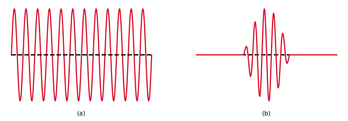

Fig. 2.7 Two examples of a probability wave: (a) a single sine wave and (b) a pulse composed of many sine waves.#
Werner Heisenberg developed a theoretical framework for this inherent “fuzziness” of the physical world. The product of the uncertainty in the position and momentum must be equal to or larger than \(\hbar/2\) and is known as Heisenberg’s uncertainty principle. A similar statement relates the uncertainty of energy and time measurements. Together they are described by
Exercise 2.7
What is the minimum speed and kinetic energy of an electron in a hydrogen atom?
The minimum speed and kinetic energy is determined using uncertainty principle for the electron’s momentum \(p_e\) and position \(\Delta x_e\). The minimum speed is given as
where the momentum is determined using the de Broglie wavelength (Eq. (2.16)).
The minimum kinetic energy is calculated using the equation for kinetic energy using the minimum speed, or
from scipy.constants import hbar, eV, physical_constants

a_o = physical_constants['Bohr radius'][0] #Bohr radius of hydrogen atom; Delta x
p_e = hbar/a_o #uncertainty in the electron's momentum p

v_min = p_e/m_e #minimum speed of the electron
K_min = p_e**2/(2*m_e) #minimum KE of the electron
#eV = 1.602176634e-19 #J in 1 eV

print("The minimum speed of the electron is %1.2e m/s or %1.3fc." % (v_min,v_min/c))
print("The minimum KE of the electron is %1.2e J or %2.1f eV" % (K_min,K_min/eV))
The minimum speed of the electron is 2.19e+06 m/s or 0.007c.
The minimum KE of the electron is 2.18e-18 J or 13.6 eV
2.4.3. Quantum Mechanical Tunneling#
Light changes its behavior at boundary transitions, where this is most easily seen for a light beam traveling from a prism (glass) into air. The light may undergo total internal reflection if its incident angle is greater than a critical angle \(\theta_c\) that is determined by the indices of refraction of the glass and air. The critical angle \(\theta_c\) can be derived from Snell’s law to get
The electromagnetic wave does enter the air, but it dies away exponentially (i.e., becomes evanescent). When another prism is placed next to the first, then the evanescent wave can begin propagating into the second prism without passing through the air gap between them. Photons have tunneled from one prism to another. The limitation to this effect is through Heisenberg’s uncertainty principle, where the location of a particle (i.e., photon) cannot be determined with an uncertainty less than its wavelength. For barriers that are only a few wavelengths wide, a particle can suddenly appear on the other side. Barrier penetration is important for radioactive decay and inside stars, where nuclear fusion rates depend upon tunneling.
Fig. 2.8 Mechanical tunneling (barrier penetration) of a particle traveling to the right. Image Credit: OpenStax:University Physics.#
2.4.4. Schrödinger’s Equation and the Quantum Mechanical Atom#
Heisenberg’s uncertainty principle prevents the use of classical models to treat the electron-proton like a planetary system. Instead, the electron orbits within a cloud of probability (i.e., orbital) where the more “dense” regions corresponding to where the electron is most likely to be found. In 1926, Erwin Schrödinger developed a wave equation that can be solved for the probability waves that describe the allowed values of a particle state (e.g., energy, momentum, etc.) and its propagation through space.
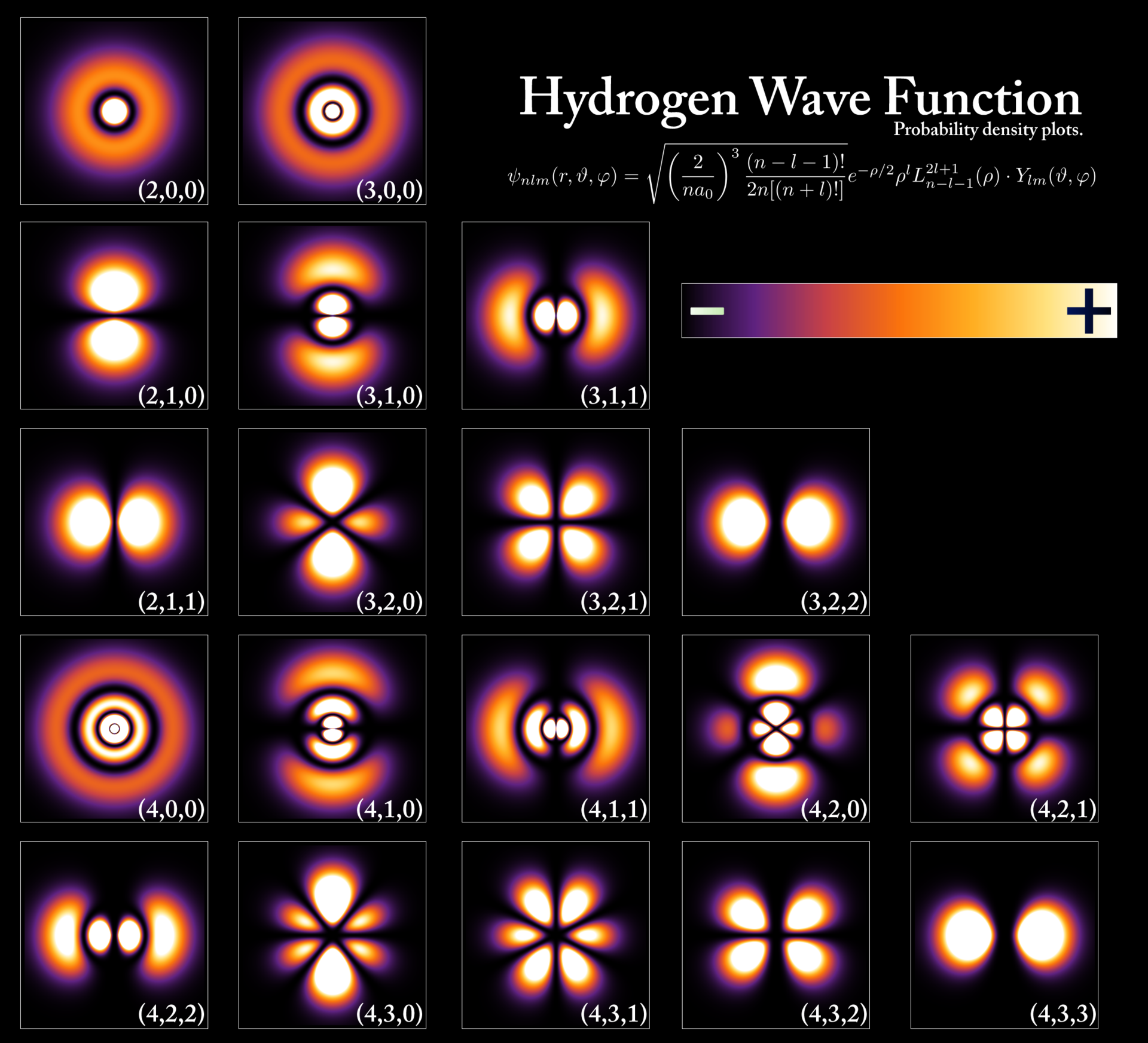
Fig. 2.9 Electron orbitals of the hydrogen atom. Image Credit: Wikipedia:Atomic orbital.#
The Schrödinger equation can be solved analytically for the hydrogen atom and it produces the same set of allowed energies obtained by Bohr. However, Schrödinger found that two additional quantum numbers \(\ell\) and \(m_\ell\) are required for a complete description of the electron orbitals. The principal quantum number \(n\) determines the energy level, where these quantum numbers describe the angular momentum vector L of the atom. The magnitude of the angular momentum \(L\) are
where \(\ell = \{0,\ldots,n-1 \}\). Early spectroscopists categorized some elements based on their alkali metal spectroscopic lines described as sharp, principal, diffuse, and fundamental and this historical nomenclature corresponded with \(\ell = 0,1,2,3\). The letters continues alphabetically where \(\ell = 4\rightarrow g\), \(\ell = 5\rightarrow h\), and so on (omitting \(j\)). Chemists now use a nomenclature that includes both the principal and angular momentum quantum numbers together (e.g., \(n\ell\)). For example, (\(n=2\), \(\ell=1\)) corresponds to \(2p\).
The \(z\)-component of the angular momentum vector \(L_z\) can assume only particular values designated by the quantum number \(m_\ell\) (i.e., \(L=m_\ell\hbar\)), which ranges from \(-\ell\) to \(+\ell\) resulting in \(2\ell +1\) possible integers. For isolated hydrogen atoms, there is not a preferred direction for the angular momentum vector to point and thus, a degeneracy exists with respect to the energy (i.e., the electron has the same energy independent of \(\ell\) and \(m_\ell\)) and will produce the same spectral line.
However, hydrogen gas in a star is not isolated and the electrons will feel the effect of the stellar magnetic field. Due to the external magnetic field the energy levels are no longer degenerate and the spectral lines are observed to split. The simplest case is described by the Zeeman effect, where the \(2p\) orbital is split into three lines; \(p=1\) and \(m_\ell = \{-1,0,+1\}\). The \(m_\ell = 0\) line appears at a frequency \(\nu_o\) that corresponds to the spectral line in the absence of the magnetic field. The other two lines are produced depending on the magnetic field strength \(B\) and reduced mass \(\mu\) to produce the frequencies
Today, the Zeeman effect is used to monitor the magnetic field of the Sun by taking spectra near sunspots. Interstellar clouds may contain very weak magnetic fields (\(B\approx 2\times 10^{-10}\;{\rm T}\)), where astronomers have been able to measure this magnetic field. The magnetic field strength of interstellar clouds depends on the number density \(n_{\rm H}\) of cloud particles, where the magenetic field strength of diffuse clouds \((n_{\rm H} < 300\ {\rm cm^{-3}})\) ranges from \({\sim}1-10\ {\rm \mu G}\) (Crutcher et al. (2010)).
Note
Another commonly used unit of magnetic field strength is gauss, where \(\rm 1\ G = 10^{−4}\ T\).
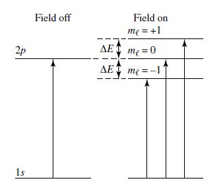
Fig. 2.10 Splitting of absorption lines by the Zeeman effect. Image Credit: Carroll & Ostlie (2007).#
Exercise 2.8
Calculate the change in frequency under the magnetic field of an interstellar cloud using the mass of the electron for the reduced mass (\(\mu = m_e\)).
The change in frequency \(\Delta\nu\) can be calculated as from the last term in Eq. (2.20), assuming that the magnetic field strength within an interstellar cloud is \(B = 2\times 10^{-10}\ {\rm T} = 2\ {\rm \mu G}\). Using mass of the electron for the reduced mass, we get
from scipy.constants import elementary_charge, m_e
def calc_Zeeman_freq(B,mu):
    #B = magnetic field strength in Tesla (T)
    #mu = reduced mass
    return q_e*B/(4*np.pi*mu) #returns frequency in Hz

q_e = elementary_charge #1.60217662e-19 #Coulombs; electron charge
B_IC = 2e-10 #magnetic field of interstellar cloud
delta_nu = calc_Zeeman_freq(B_IC,m_e)
print("The change in frequency from the Zeeman effect is %1.1f Hz." % delta_nu)
The change in frequency from the Zeeman effect is 2.8 Hz.
2.4.5. Spin and the Pauli Exclusion Principle#
More complicated patterns of magnetic field splitting led physicists to discover another quantum number related to the spin angular momentum S of an electron. This is not a classical top-like rotation but purely a quantum effect. The spin vector has a constant magnitude
with a \(z\)-component \(S_z = m_s\hbar\) and \(m_s = \pm 1/2\). The quantum state of an electron can be described by four quantum numbers, but no two electrons can occupy the same quantum state, Pauli Exclusion principle. This provided an explanation for the properties of the period table of elements. However, there wasn’t a first principles reasoning for why a fourth quantum number was needed.
Quantum mechanics was at odds with Schrödinger’s (non-relativistic) wave equation and Einstein’s theory of special relativity. Paul Dirac worked to combine the two theories and succeeded in writing a relativistic wave equation for the electron that naturally included the spin of the electron. His relativistic wave equation extended the Pauli exclusion principle by dividing the world of particles into two groups: fermions and bosons.
Fermions are odd-integer half-spin particles (e.g., \(\frac{1}{2}\hbar\), \(\frac{3}{2}\hbar\), \(\ldots\)) such as electrons, protons, and neutrons. Fermions obey the Pauli exclusion principle, which explains the structure of white dwarfs and neutron stars.
Bosons are integer spin particles (e.g., 0, \(\hbar\), \(2\hbar\), \(\ldots\)) such as photons. Bosons do not obey the Pauli exclusion principle.
The Dirac equation also predicted the existence of antiparticles. A particle differs from its antiparticle in its charge and magnetic moment (e.g., electron \(e^-\) and positron \(e^+\)); all other properties are the same. Pairs of particles and antiparticles may be created from the energy of gamma-ray photons (e.g., \(\gamma \rightarrow e^- + e^+\)) or annihilate each other to produce gamma-rays (e.g., \(e^- + e^+ \rightarrow \gamma\)). Such processes play a role for fusion inside of stars and in the evaporation of black holes.
2.4.6. The Complex Spectra of Atoms#
Four quantum numbers (\(n\), \(\ell\), \(m_\ell\), and \(m_s\)) describe a quantum state for each electron in an atom, where external magnetic fields (and other electromagnetic interactions) increase the number of possible energy levels. Even though there are a large number of possible states to make a transition, some transitions are restricted, where Nature imposes a set of selection rules that determines the allowed and forbidden transitions. The allowed transitions can happen spontaneously on timescales of \(10^{-8}\) s, while the requirement of \(\Delta \ell = \pm 1\) prevents transition from \(F\) to \(P\).
Fig. 2.11 Some of the electronic energy levels of the helium atom. Image Credit: hyperphysics.#
The Zeeman effect shows only three transitions occur between \(1s\) and \(2p\) energy levels because of selection rules requiring \(\Delta m_\ell = 0\) or \(\pm 1\) and forbidding transitions if both orbitals have \(m_\ell = 0\). Similar to quantum tunneling, there remains a small but finite probability for forbidden transitions to occur and they require much longer timescales. Collisions between atoms trigger transitions and can compete with spontaneous transitions. Thus, very low gas densities are required to obtain a sufficient signal to measure the forbidden transitions. In the diffuse interstellar medium or the outer atmospheres of stars, this condition is met.
2.5. Homework#
Problem 1
Barnard’s star is an orange star in the constellation Ophiuchus. It has the largest known proper motion \(\mu = 10.3934^{\prime\prime}\)/yr and the fourth-largest parallax angle \(p = 0.5469759^{\prime\prime}\) (Gaia Collaboration). The H\(\alpha\) absorption line is observed at 656.034 nm when measured from the ground.
(a) Determine the radial velocity of Barnard’s star.
(b) Determine the transverse velocity of Barnard’s star.
(c) Calculate the speed of Barnard’s star through space.
Problem 2
The Sun’s spectrum contains two spectral lines (Sodium D lines) 588.997 nm and 589.594 nm.
(a) If a diffraction grating with 300 lines per millimeter is used to measure the Sodium D lines, what is the angle between the second-order spectra for each of the wavelengths?
(b) How many lines must the grating have to resolve the sodium D lines?
Problem 3
The ejection of an electron leaves a grain of dust with a positive charge, which leads to heating within an interstellar cloud. If the average energy of the ejected electron is about 5 eV and the process is particularly effective for UV photons (\(\lambda \approx 100\) nm), estimate the work function \(\phi\) of a typical dust grain.
Problem 4
Consider the case of a “collision” between a photon and a free proton (initially at rest) given a scattering angle \(\theta=90^\circ\).
(a) What is the characteristic change in the wavelength of the scattered photon (in nm)?
(b) How does this compare with the Compton wavelength, \(\lambda_C\).
Problem 5
To demonstrate the relative strengths of the electrical and gravitational forces between the electron and proton in the Bohr atom, suppose the hydrogen atom were held together solely by gravity. Determine the radius of the ground-state orbit (in nm and AU) and the energy of the ground state (in eV).
Problem 6
Calculate the energies and vacuum wavelengths of all possible photons that are emitted when the electron cascades from the \(n=3\) to the ground state of the hydrogen atom.
Problem 7
An electron in an old TV set reaches a speed of about \(5\times 10^7\) m/s before it hits the screen. What is the wavelength of this electron?
Problem 8
A White dwarf is a very dense object, with its ions and electrons packed extremely close together. Each electron may be considered to be located within a region of size \(\Delta x \approx 1.5 \times 10^{-12}\) m. Estimate the minimum speed of the electron using Heisenberg’s uncertainty principle. Do you think that the effects of relativity will be important?
Problem 9
An electron spends roughly \(10^{-8}\) s in the first excited state of the hydrogen atom before spontaneously decaying back to the ground state.
(a) Determine the uncertainty \(\Delta E\) in the energy of the first excited state.
(b) Calculate the uncertainty \(\Delta \lambda\) in the wavelength of the photon for this transition. Why can you assume that \(\Delta E = 0\) for the ground state?