Student Participation (Spring 2024)#
Students will work in pairs to produce summaries of each class meeting. These summaries should list the main topics discussed and emphasized ideas/examples during the respective lecture. Students are encouraged to be as detailed as possible without being overly verbose. The summaries should be submitted as a pull request from your forked repository before the next class meeting.
Jan 8#
Class Overview#
This class uses the first half of An Introduction to Modern Astrophysics by Carroll & Ostlie (2007)
Cosmology covers the latter half
Class calender shows all expected exams and assighments due, and can be found here.
Syllabus
Course includes 2 presentations and 3 exams.
follows this grading split
Relative Weights
Teaching Pres. 10%
Review Pres. 20%
Exams 15% (each)
Participation 10%
Homework 15%
Exams
Two closed-book exams and one take-home
exams will be a mixture of multiple choice and free repsonse questions
should resemble some homework questions
Course Presentations
requires the student to teach a data analysis or modeling skill using an open-source python package to the instructor and other students.
uses Astropy
10 minutes long 2. Pairs of students will also present a full review of a topic within astrophysics.
20 minutes long with a 5 min period for questions.
Grading Scale
A 88 – 100%
B 77 – 87%
C 66 – 76%
D 55 – 65%
F <54%
Office hours
11am – 12 pm, MWF,
10:00 – 11:00am TR,
Course website
all the course website can be viewed in the code version of the website
useful for seeing how billy took certain notes
GitHub accounts
to have a personal version of the raw version of the notes, you must fork the orignal repository
https://github.com/saturnaxis/ModernAstro
to submit notes
in word or collab, write the notes
in the forked repository go to the appendix file and open the Student_Summaries.ipynb file
click the pencil icon to edit the file in github.dev
then copy your written notes into the github.dev version of the code
If you didnt write your notes in collab, you can instead write the notes in the github.dev version of the notes
Once you are done writing the notes, click the Source Control icon to commit & push the updated version of code to youre forked repository
Look to see if the notes look correct, if they do, submit a pull request to get it added to main repository
Billy will get an email and push the request if the notes looks passable
Done
tip when wirting notes collaborative
it is much easier to have one google collab and then share it with the person you are paired to, rather than using word or anything else
Jan 10#
Continuous Spectrum of Light Part I#
1.1 Stellar Parallax
Trigonometric parallax: measurement of angular displacement of an object from two different vantage points creating a known baseline distance \(B\) between observers. \(d = B/tan(p)\). \(tan(p)\) comes from small angle approximations, so we can use \(p"\) (” standing for arcseconds) for angle values smaller than \(1\) arcsecond.
The angles at which these stars move relative to the much more distant stars in the background are very small.
\(3600\) arcseconds per \(1\) degree because of \(1/60/60 = 1/3600\). You have \(360\) degrees of sky, split \(1\) of those degrees into \(60\) pieces, giving you \(60\) arcminutes. Then you take \(1\) of those arcminutes and split that into \(60\) pieces, giving you \(60\) arcseconds.
Arcseconds are very small amounts of angle, and can be divided further for smaller movements across the night sky. Example: Proxima Centauri has a parallax angle of less than \(1"\).
We measure stellar distances in units of parsecs (parallax-seconds), 206,265 AU per parsec (great distance).
First successful measurement of stellar parallax in 1838 by Fredrich Bessel (1784-1846).
\(1 pc = 3.2615638 ly\)
Objects with small parallax angles have interfering conditions such as geologic tremors or atmospheric turbulence which make it hard to find accurate angles. Space missions such as Hipparcos don’t have this problem.
1.2 The Magnitude Scale
1.2.1 Apparent Magnitude
Hipparchus compiled a list of ~850 stars (some found by Persians before, he just added to the list and listed previously known ones) and compared their brightness. Later examinations of his scale showed that it was logarithmic because the human eye perceives the brightness of objects logarithmically.
Example: if a bright light source were \(6\) times brighter than another, the human eye will determine the brighter object as approximately twice the brightness of the other.
This means that the difference in brightness between two different magnitude stars is \(100^{(m2-m1)/5}= ΔB\). Two stars separated by \(1\) magnitude have a difference in brightness of \(2.512\) times, or \(100^{1/5}\). Two stars separated by 5 magnitudes have \(100\) times difference in brightness.
1.2.2 Flux, Luminosity, and the Inverse Square Law
Radiant flux \(F\) is the brightness of a star measured by the total amount of radiation at all wavelengths that cross a unit of area per unit time. Definition depends on the energy emitted per second at the stellar surface (intrinsic luminosity \(L\))
Luminosity \(L\) is distributed uniformly across the surface area of a shell of radius \(r\) surrounding a star.
This is the well-known inverse square law for light. The \(4π\) factor is not necessarily needed as the radiant flux of some stars are given relative to the Solar Luminosity (L_sol) and the Earth-Sun distance (r_earth).
\(F = L/4πr^2\)
1.2.3 Flux Ratios and Apparent Magnitude
Absolute magnitude M of a star is the apparent magnitude a star would have if it were located at a distance of \(10 pc\). We can find the ratio of their flux to be, \({\frac{F_2}{F_1}} = 100^{m_1-m_2/5}\)
Logarithm of both sides of the flux ratio above gives an alternative form: \(m_1-m_2 = -2.5log_{10}{\frac{F_2}{F_1}}\)
1.2.4 Absolute Magnitude and the Distance Modulus
Distance modulus: \(m-M = 5log_{10}(d)-5 = 5log_{10}{\frac{d}{10 parsecs}}\)
How bright a star would be if it were \(10 pc\) away is called the absolute magnitude
Multiply the \(10\) over from \(d/10 pc = 10^{(m-M)/5}\) and that gives you the +5 being added to the two magnitudes in the exponent
Goes from \(10^{-6}\) to \(10^{-7}\) because the \(d/10\) you are just dividing by \(10^{1}\) to make a more negative exponent.
M_Sun needs to be written out as “Sun” in the subscript, otherwise putting a circle dot would make the quantity the mass of the Sun.
1.3 The Wave Nature of Light
1.3.1 The Speed of Light
Ole Roemer determined that the speed of light was finite by extensive measurements of Jupiter’s moons eclipsing when Earth was near the opposite side of the Sun compared to Jupiter.
He used Kepler’s original third law without universal gravitation. It wasn’t until 1761 until we found out the distance of an AU, so that also hampered the mathematics needed to calculate the speed of light.
1.3.2 Young’s Double-Slit Experiment
Christian Huygens (1629-1695) suggested that light was and behaved similarly to waves, with wavelengths, crests, and troughs.
c = (wavelength)(frequency)
Thomas Young’s double-slit experiment: two waves of light interfering with each other going through the slits. Destructive interference occurs when the peaks and troughs of the light wave cancel eachother, making darker parts on the screen. Constructive interference occurs when there are brighter fringes.
1.3.3 Maxwell’s Electromagnetic Wave Theory
Breakthrough in nature of light waves from Scottish mathematical physicist James Clerk Maxwell (1831-1879).
Electromagnetic waves are transverse waves with an Electric field E and magnetic field B component.
1.3.4 The Poynting Vector and Radiation Pressure
EM waves carry both energy and momentum in the direction of propagation. The rate at which energy is carried by a light wave is described by the Poynting vector.
\(S=\frac{1}{\mu_0}ExB\)
The Poynting vector is reliant on the cross product of the electric and magnetic field components of the EM wave. The units are in watts per meter squared \(W m^{-2}\).
When EM waves reflect off of a surface at a certain angle \(θ\) because it is conserving momentum upon impact, causing it to go in another direction.
Jan 15 (MLK Day)#
No Class#
Jan 17#
Continuous Spectrum of Light Part II#
1.41 The Connection between Color and Temperature
The start of thermodynamics occured in the early 19th century
was found out that all objects emit light all all wavelenghts with varying effecency
blackbodys
objects that absorb all of the incident light and re-radiates the energy with a characteristic spectrum (blackbody radiation)
blackbody radiation is the energy
stars are blackbodys (not perfect ones like expected though)
They produce a continous spectrum with some energy are at all wavelenghts
Wiens displacment law describes a relationship between temperature and color
1.42 The Stefan-Boltzmann Equation
Spectral energy density increases for higher surface tempearture (more intensity for higher temperature)
Stefan-Boltzamnn found an equation for luminoisty
derived from thermodynamics and Maxwells formula for radiation pressure
1.5.1 Rayleigh- Jeans and wiens Approximation
based on Maxwells equations, Rayleigh derived an approximate for wavlenghts and temperature.
messes up at at a limit of \(\lambda\) (i.e., \( \lim_{\lambda\rightarrow 0} B_\lambda(T) = \infty\)).
called the ultraviolet castastophe, or Rayleigh Jeans law
At the same time, Wien worked on his own approximation
\(a\) and \(b\) were determined by a best-fit to the experimental data.
1.5.2. Planck’s Function for the Blackbody Radiation Curve
Planck found a better more refined version of Wiens approximation
\[B_\lambda(T) = \frac{a\lambda^{-5}}{e^{\frac{b}{\lambda T}}-1}. \qquad \text{(Planck Function)}\]Subtracted one from the exponital function in Wiens approximation
Allows approximation fit the blackbody curves for both long and short wavelengths.
\(a=2hc^2\) and \(b= (hc)/k\).
1.5.3. The Planck Function and Astrophysics
in spherical cooridantes the radiant energy given wavelenght per unit time can be expressed from an element of surface area dA as $\(L_\lambda d\lambda = \int \int \int B_\lambda(T)d\lambda dA \cos \theta \sin \theta d\theta d\phi.\)$
1.6. The Color Index
Brightness measured over all wavelenghts is called bolometric magnitude
in practice, scientist measure radiant flux through specific filters that only allow a certain wavelenght to pass
1.6.1 UBV Wavelength Filters
A stars color can be precisely measured using a filter that permits a narrow range of wavelenghts to to pass through. Using this, Astromers developed a standard UBV photmetric system to classify stars.
(U) Ultraviolet magnitude centered at 365 +_ 65 mm
(B) Blue magnitude 440 +_ 98mm
(V) Visible 550 +- 89 mm
1.6.2 Color indices and the Bolometric Correction
Color index
difference between stars apparent magnitude in each of hte standard wavelenghts
and
A star is blue is if \(M_b\) is is brighter than \(M_v\) or \(B-V\) is brigher
The difference between a star’s bolometric magnitude and its visual magnitude is called the bolometric correction \(BC\)
Apparent magnitudes corresponding to each filters can be determines through the apparent flux compared to another star.
A &sensitivity function \(S(λ)\) describes how much a star’s flux can be detected for a given wawvelength.
A star’s magnitude with respect to a given filter X is
\[m_X = -2.5 \log_{10}\left(\int_0^\infty F_\lambda S_X d\lambda\right) + C_X,\]
Color indices (U-B or B-V) are deteremed though the fulx ratio,
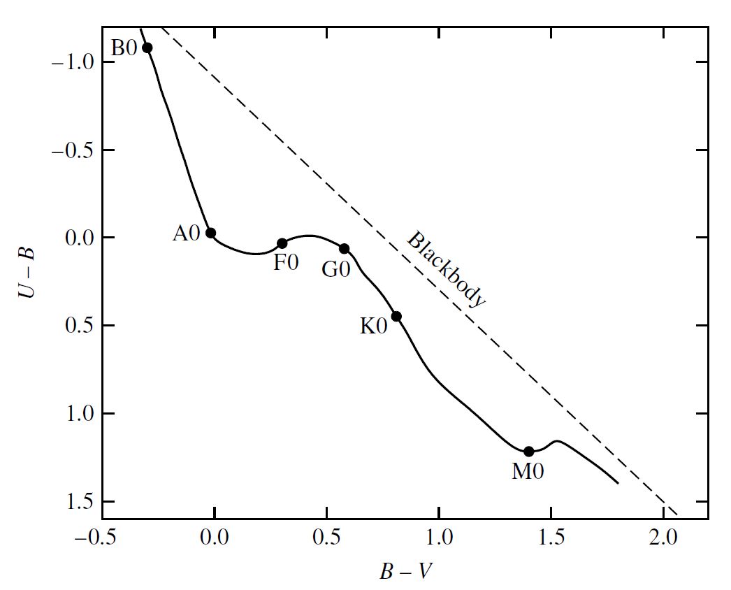
1.6.3. The Color-Color-Diagram
Color diagram
shows relation bewteen the \(U-B\) and \(B-V\) indices for main sequence stars here
resmembles a H-R diagram
stars are fueled by nuclear fusion of hydrogen nuclei
80 - 90 % of al stars lie on the main sequence
the Color diagram shows stars are not perfect blackbodies
the relationship on the graph would be linear
very hot stars tend to fit the black body model
as light travles to the stars core, it is differentially absorbed as a function of the wavelength of light and the star’s temperature.
Jan 22#
Interaction of Matter and Light Part I#
2.1 Spectural Lines
In the year 1800 William Wollaston shown a number of dark spectural lines were present within the rainbow-like spectrum.
2.1.1. Kirchoff’s Laws
Thee foundation of spectroscopy and moderny chemistry were established in the 1800s with Robert Bunsen and Gustav Kirchoff.
In the 1860 Kirchiff and Bunsen developed the idea that every element produces it’s own pattern of spectural lines and thus the elements have “fingerprints.”
A hot dense gas or hot solid object produces a continuous specturm with no dark spectural lines
A hot diffuse gas produces bright spectural lines (emission lines).
A cool, diffuse gas in front of a source of a continuous spectrum produces dark spectral lines (absorption lines) in the continuous spectrum.
2.1.2. Applications of Stellar Spectral Data
Radial Velovity (\(v_r\)):
The rest wavelength (\(\lambda_{\rm rest}\)) or the hydrogen spectral line (\({\rm H}_\alpha \)) is 656.281 nm (in air).
proper motion (\(\mu\)) is perpendicular to line-of-sight.
Combining the proper motion with a known distance r, the transverse velocity (\(v_\theta\)) can be determined (\(v_\theta = r\mu\)).
The average speed of stars in the solar neighborhood is about 25 km/s, where the measurement of a star’s radial velocity is also complicated by the motion of the Earth (29.8 km/s) around the Sun.
Astronomers correct for this motion by subtracting the component of Earth’s orbital velocity along the line-of-sight from the star’s measured radial velocity
2.1.3 Spectrographs
Astronomers use spectographs to measure the radial velocity of exoplanets, stars, and galaxies.
Modern spectrographs collimate the incoming starlight onto a mirrior and split into a constituent colors using a diffraction grating
Different wavelengths have their maxima occurring at different angles (𝜃) by: \(d\sin \theta = n\lambda\)
d is the slit spacing of the grating, n is the order of the spectrum and 𝛳 is measured relative the line perpendicular to the grating.
The smallest measurable difference in wavelength (\(\Delta \lambda\))depends on the order and the total number of lines (N), through:
Where λ is either of closely spaced wavelengths. The ration λ/Δλ is one way to express the resolving power of the grating.
2.2 Photons
photons: bundles of energy used to describe light.
The energy is described in terms of Planck’s constant h and is recognized as a fundamental constant of nature like the speed of light c.
quantum mechanics: description of matter and energy which uses Planck’s discovery of energy quantization.
2.2.1. The Photoelectric Effect
photoelectric effect: describes the light energy necessary to eject electrons from a metal surface.
The electrons with the highest kinetic energy (\(K_{max}\)) originate from the surface of the metal. (does not depend on the light intensity.)
A higher intensity of light increases the number of electrons ejected, but not their maximum kinetic energy.
The value of \(K_{max}\) varies with the frequency of the light and each metal has a characteristic cutoff frequency and wavelength.
Energy of a photon: \begin{align} E_{\rm photon} = h\nu = \frac{hc}{\lambda}. \end{align}
Maximum kinetic energy of the ejected electrons:
2.2.2 The Compton Effect
Arthur Compton measured the change in the wavelength of X-ray photons as they were scattered by free electrons.
The energy of a photon is related to its momentum (p) by:
During a collision of a proton and a free electron, the electron is scattered by an angle \(\varphi\), while the photon is scattered by an angle \(\theta\).
The photon’s energy is reduced and the wavelength is increased due to the energy exchange.
The change in wavelength is the difference between the final and initial wavelength and can be expressed as:
where \(m_e\) is the mass of the electron.
The prefactor \(h/m_e c\) is called the Compton wavelength \(\lambda_C\).
Compton’s experiment provided evidence that photons carry momentum.
Jan 24#
Interaction of Matter and Light Part II#
2.3.1 The structure of the atom
2.3.2 The Wavelength of Hydrogen
The spectral lines are described by their wavelength and categorized isong greek letters (\(\alpha , \beta\)…)
Balmer equation decribes the wavelengths for hydrogen spectral lines
\[ \lambda = \frac{1}{R_H} \left(\frac{4n^2}{n^2 -4}\right) \]where \(n\) is an integer greater than 2. and \(R_H = 1.09677583 \times 10^7 \pm 1.3\ m^{-1}\) and known as the Ryberg constant. The more general form of the equation, where \(m<n\),
\[ \lambda = \frac{1}{R_H} \left(\frac{m^2n^2}{n^2 - m^2}\right) \]Note: this is only for hydrogen
2.3.3 Bohr’s Semiclassical Atom this interpretation is out of date
To analyze the interactions between a proton and electron, we start with Coulomb’s law (\(q_n\) is the 2 charges, and are seperated by \(r\).)
\[F = \frac{1}{4\pi \epsilon_0} \frac{q_1q_2}{r^2}\]\(epsilon_0\) is the permitivity of free space. Eventually, we get to the energy (in terms of fundamental constants) is
\[E_n = -\frac{\mu e^4}{32\pi^2\epsilon_0^2\hbar^2}\frac{1}{n^2} = \frac{-13.6 \text{eV}}{n^2}\]If you assume the energy required between levels is the energy of a photon \(e_{photon} = \frac{hc}{\lambda} = E_{high} - E_{low}\), we have (hc = 1240 eV nm);
\[\lambda = \frac{hc}{13.6 \text{ev}}\frac{n^2_{high}n^2_{low}}{n^2_{high} - n^2_{low}}\]Notice how similar this is to the 2nd equation
2.4 Quantum Mechanics and Wave-Particle Duality
2.4.1 de Brogolie’s Wavelength and Frequency
Einstein special relativity tells us that photons carry both energy \(E\) and momentum \(p\), which can be related to a frequency \(\nu\) (or \(v\) if you’re Sterling) and wavelength \(\lambda\) by,
\[\nu = \frac{E}{h} \text{and,}\]\[\lambda = \frac{h}{p}\]2.4.2 Heisenberg’s Uncertainty Principle
Says you can’t know, with a high degree of certainty, at the same time, the position and momentum OR, the energy and the time. The equations showing this are,
\[\Delta x \Delta p \approx \hbar \text{ and } \Delta E \Delta t \approx \hbar\]2.4.3. Quantum Mechanical Tunneling
Light exhibits total internal reflection when transitioning between media with differing refractive indices, like from glass to air.
Tunneling phenomena, where particles traverse barriers without passing through, are explained by the wave-particle duality and Heisenberg’s uncertainty principle.
2.4.4. Schrödinger’s Equation and the Quantum Mechanical Atom
Schrödinger’s wave equation describes electron behavior in atoms, revealing probability distributions of electron positions.
Quantum numbers like ℓ and mℓ characterize electron orbitals, crucial for understanding phenomena like the Zeeman effect caused by external magnetic fields.
2.4.5. Spin and the Pauli Exclusion Principle
Electron spin introduces a fourth quantum number, underlying the Pauli Exclusion Principle that prohibits identical quantum states for electrons.
Paul Dirac’s relativistic wave equation unified quantum mechanics and special relativity, predicting fermions, bosons, and the existence of antiparticles.
2.4.6. The Complex Spectra of Atoms
Quantum numbers define electron states within atoms, influencing their response to external electromagnetic fields and determining allowed transitions.
Selection rules govern these transitions, dictating the observed spectroscopic behavior in atoms, including phenomena like the Zeeman effect and forbidden transitions in low-density environments.
Jan 29#
Telescopes Part I#
3.1 Basic Optics
3.1.1 Refraction and Reflection
First telescope developed by Hans Lippershey in 1608 and Gallileo Gallilei was first to use one for astronomical viewing in 1609. In 1671, Isaax Newton make reflecting telescope which helps remove chromatic aberration common with lenses.
Two types are reflecting and refracting.
Reflecting Telescope uses a mirror to reflect light.
Refracting Telescope uses lens to refract light.
Both of these methods bend light to form an image.
Refraction works by Snell’s law described by
\[n_1\sin\theta_1 = n_2\sin\theta_2\]where \(n_1,\theta_1\) are the refractive index for the first material and \(n_2,\theta_2\) are for the second material.
The index of refraction is both material dependent and wavelength dependent by \(n_{\lambda} = c/v_{\lambda} \), where \(v_{\lambda} \) is the speed of light in that medium. The frequency of the wave remains unchanged.
The lenses for refracting telescopes are formed from glass and are either converging or diverging.
Converging lenses focus the light to a certain point on the optical axis known as the Focal Point and the length from the lens to this point is called the Focal length.
Diverging Lenses diverge the light away from the optical axis, thus the focal point is on the same side of the lens as the light. (Negative focal length vs positive for converging).
The Lens Maker’s Formula gives the formula for finding the focal length of a lens by:
\[f_{\lambda} = \frac{1}{n_{\lambda}-1}\frac{R_1R_2}{R_1+R_2}\]
3.1.2 Focal Plane
To record an image, a detector must be placed on the Focal Plane of the telescope (plane passing through focal point). On axis point sources of light will converge on the focal point while other sources will focus approiximately on a distance y above the axis by:
\[ y = f\tan\theta\]\[ y \approx f\theta \]This leads to plate scale \( \frac{d\theta}{dy} = \frac{1}{f} \) which connects angular separation of objects in sky by their linear separation in the images.
3.1.3 Resolution and the Rayleigh Criterion
There is a fundamental limit to our ability to resolve two objects due to the defraction of the light. This is related to the single slit diffraction pattern produced by light passing through a slit of width D.
Any ray passing through an aperature (opening) can be though of as being associated with another ray separated by a distance D/2 and arriving at the same point. If they are half wavelength out of phase then destructive interferrence will occur which leads to
\[D\sin\theta = m\lambda\]where \(m=1,2,3...\) for the dark fringes due to destructive interferrence. This produces a series of concentric fringes known as the Airy Disk.
Now, two sources that are clsoe together will have diffrwaction fringes that overlap making it impossible to resolve. Considered unresolvable if max of one falls within minimum of the other. This is known as the Rayleigh Criterion. Assumign angular separation is small, we get
\[\theta_{min} = 1.22\frac{\lambda}{D}\]for a circular apperature of a telescope with diameter D observing a wavelength of \(\lambda\).
Ground based telescopes rarely approach this due to atmospheric turbulence.
3.1.4 Aberrations
Refracting telescopes suffere chromatic aberrations due to the wavelength dependent diffraction, which causes color fringing.
Aberrations can be caused by shape imperfetions of the lens or mirror as well. This is called spherical aberration.
Coma produces elongated images fo point sources.
Astigamatism caused when different parts of mirror or lens converge at different focal points. Fixing this can cause other problems such as a cruvature field.
3.1.5 Image Brightness
Determined by intensity of the collected light (number of light rays going into aperature).
Also determined by the focal ratio of the telescope (how many light rays being imaged after they are spread apart by the aperature). This is given by
\[ F = f/D \]Illumination determines time needed to collect enough light to form image.
3.2 Optical telescopes
3.2.1 Refracting Telescopes
Use two lenes with two focal lengths (\(f_{obj}\) for objective lens and \(f_{eye}\) for eye piece lens). The angular magnification of the image for a refacting telescope can be determined using their ratio
\[ m = \frac{f_{obj}}{f_{eye}} \]Defects in the shape of the lens must be small, on the order of \(\approx \lambda/20\) .
3.2.2 Reflecting Telescope
Replaces objective lens with a mirror that reflects the light into the eye piece instead of refracting. Requires much less precision since the light doesn’t pass through the lens. A large mirror collects the light at the bottom while a secondary mirror near the top or middle focuses the light into the eye piece.
Newtonian Telescopes have eyepice or detector far above the center of mass of the telescope which causes problems mechanically due to the torque.
Cassegrain Since the secondary mirror blocks a point near the center of the objective mirror, a hole can be put here where the secondary mirror can refelct light into eyepice in the bottom of the etelscope.
Ritchey-Chretien uses hyperbolic mirror instead of parabolic which gives a larger field of view and also elimnates off axis optical errors.
If instruments are too large, a series of mirrors reflect the light to a Coude room where they can be processed out of the way.
Schmidt-Cassegrain uses a spheroidal primary mirror and corrective lenses to reduce aberrations and also has a wider field of view.
3.2.3 Adaptive Optics
Use of rubber mirrors that can be moved to adapt and correct to the changing shape of wavefronts of light due to the atmosphere. To do this, monitors guide star that is near the object to guage the change in the atmosphere.
3.2.4 Space-Based Observatories
Telescopes placed in space to remove the effects of the atmosphere. These are much more precise than ground based but are much more expensive to make.
3.2.5 Electronic Detectors
Photographic plates were used first by astronomers to save images from telescopes.
Once CCD (chareg coupled device) were invented they dominated telescope imaging as they are nuch more efficient and can collect almost 100 percent of incident light. They work by collecting the electrons that are excieted due to a photon striking them into a collector and detecting them. Number of electrons collected in each pixel determines the brightness of the image.
Very bright objects require quick shudders to prevent pixels from saturating (electron collectors are full and thus cannot measure the image accurately anymore since there is little differences inbetween pixels.)
Jan 31#
Telescopes Part II#
3.3 Radio Telescopes
By the 1930s, companies such as Bell Labs, were interested in short wave (λ=10 -20 m) transmissions for use in a trans-Atlantic radio service, where properties of the atmosphere and ionesphere could introduce static to radio voice transmissions.
Radio telescopes operate differently from their optical counterpart where radio observations can be take any time of day or night. At long wavelengths, transmissions is limited by the ionesphere. Water vapor interferes with radio astronomy at shorter wavelengths, which has led to building radio observatories that conduct observations at milimiter wavelengths at very high sky.
3.3.1. Spectral Flux Density
A radio telescope uses a parabolic dish to reflect the radio energy to an antenna.
Parabolic Dish is a reflective surface used to collect or project energy such as light, sound, or radio waves.
The strength of a radio source is measured in terms of the spectral flux density \(S(\nu)\), which is the amount of energy per second (W) per unit of frequency (Hz) per unit area (\(m^2\)). Mathematicallt the power is given as
\[P = \int_A \int_\nu S(\nu)f_\nu d\nu dA, \]where \(f_\nu\) is the detector efficiency at a particular frequency \(ν\). Typycal measurements are on the order of mJy, where a larger aperture is needed to collect enough photons to be measurable.
To determine the power collected by the receiver, the spectral flux must be integrated over the telescope’s collecting area and over the detector’s bandwidth (i.e., frequency interval).
3.3.2. Improving Resolution: Large Apertures and Interferometry
The resolution of a single small radio telescope poor due to Rayleigh’s criterion because the wavelength λ is necessarily large compared to the optical regime. To obtain a comparable resolution requires a very large aperture.
The solution to improved resolution is accomplished through a technique called interferometry, which uses multiple telescopes to mimic a large aperture. For interferometry to work, astronomers utilize two radio telescopes separated by a baseline d.
For the signal to arrive at both telescopes in-phase and at a maximum intensity, the extra distance traveled to one telescope must be an integral number of wavelengths \(L=n\lambda\), where \(n=0,1,2,...\)
The pointing angle θ is then determined as
\[\sin \theta = \frac{L}{d}.\]If the signals of the two antennas are combined and a source can be accurately located.
A single has its greatest sensitivity along its pointed direction, but it also can be sensitive to radio sources at other angles.
A typical antenna pattern maximizes the symmetry in dipole radiation, where there are three regions: a main lobe, black lobe and sidelobe. The narrowness of the main lobe is referred as the half-power beam width or angular width at half of its length.
3.4. IR, UV, X-Ray, and Gamma-ray Astronomy
3.4.1. Atmospheric Windows in the EM Spectrum
Optical and radio telescopes can detect a vast majority of the radiation that reaches Earth’s surface. The primary contributor to IR absorption is water vapor, where some observatories are placed above the atmospheric water vapor to make this observations. IR observations are complicated by the background heat of the telescope and detector.
3.4.2. Observing Above the Atmosphere
In 1983, the Infrared Astronomy Satellite (IRAS) was placed in orbit 900 km above the Earth’s surface. IRAS detected dust in orbit around young stars, which was an indication of the formation of planetary systems. Other new discoveries included a dust ring surrounding Vega and the first images of the Milky Way’s core.
Shorter wavelengths require a very precise reflecting surface and it wasn’t until the Space Age could UV, X-ray, or Gamma-ray observations could be performed.
From the success of IRAS, the European space Agency followed with the Infrared Space Observatory in 1995. The Cosmic Background Explorer (COBE) was launched and operated from 1989-1993 investigating the microwave regime. COBE was followed by two more advanced spacecraft: the Wilkinson Microwave Anisotropy Probe (WMAP) operated from 2001 to 2010 and the Planck spacecraft from 2009 to 2013.
The most famous X-ray telescope Chandra has been in operation from 1999 and operates from 6.2 - 0.1 nm (0.2 - 10 keV) with an angular resolution of approximately 0.5′′.
The Compton Gamma Ray Observatory (CGRO) was a space observatory designed to detect radiation with energy from 20 keV to 30 keV.
Feb 5#
Classification of Stellar Spectra Part I#
4. The Classification of Stellar Spectra
4.1. The Formation of Spectral Lines
4.1.1. The Spectral Types of Stars
Stars were originally denoted by using capital letters from A to Z that told us about the respective strength of the hydrogen absorption lines.
This form of nomenclature was developed by Edward Pickering and William Flemming.
Antonia Maury’s version of this, using the width of spectral lines, would have made Pickering’s B stars to come before the A stars.
Annie Jump Cannon built on Maury’s work, and added subdivisions (e.g., A0-A9).
All of this resulted in the Harvard classification scheme becoming a temperature sequence with seven spectral types.
Mnemonic Examples:
Oh Be A Fine Girl/Guy, Kiss Me
Oh Boy, An F Grade Kills Me
Stars near the beginning of a given spectral type are referred to as early-type stars (e.g., A0), and those near the end are called late-type stars (e.g., A9).
A catalogue was made and named the Henry Draper Catalogue, which collected results of around 200,000 classified spectra (Betelguese is HD 39801).
Henry Draper was one of the first to photograph and classify a star based on its spectral lines.
After his death Pickering took over the supervision of photographic spectrsocopy at Harvard College Observatory.
The placement of our Sun and Vega within the spectra classifications led to two questions:
Is this a result of a compositional difference between the stars?
Are the different surface temperatures responsible for the relative strengths of the absorption lines?
Absorbtion lines are created when an atom absorbs a photon that has the energy required for the electron to make an upward transition between energy levels.
Emission lines are formed by the inverse process.
The distinction between spectra of stars with different temperatures are due to the electrons occupying different atomic orbitals in the star’s atmosphere.
The ionization of atoms complicates the details of spectral lines.
In Cannon’s classification scheme, the Balmer lines (hydrogen absorption) reach their max intensity when the effective surface temperature of a star reaches 10,000 K.
Visible neutral helium (He I) lines occur at 22,000 K (B2 stars).
Singly ionized calcium (Ca II) are most intense at 5,250 K (K0 stars).
4.1.2 The Maxwell-Boltzmann Velocity Distribution
Electronic transitions explained the existence of absorption or emission lines, but they did not explain the relative strengths of the lines. Two questions arised from this.
In what orbitals are electrons most likley to be found?
What are the relative numbers of atoms in various stages off ionization?
Question one allows us to have insight into which spectral lines we expect to be stronger than the others. Question 2 will examine the relative strengths of the spectral lines.
The answers to these questions are found in statistical mechanics.
This is a branch of Physics that studies the statistical properies of many body systems.
To understand the behavior of a system, properties such as internal energy, pressure, and density are used.
If a gas is in thermal equilibrium, the Maxwell-Boltzmann velocity distribution function describes the number density of gas particles n within a given range of speed v.
\(n_vdv = n(\frac{m}{2πkT})^{3/2}e^{-mv^2/(2kT)}4πv^2dv\)
The exponent of this function is the ratio of a gas particle’s kinetic energy to the characteristice thermal energy.
Particles above the thermal energy tend to escape, so the overall temperature and distribution remains the same.
The distribution peaks when the particle energies are equal at a most probable speed of
\(v_{mp}= \sqrt{\frac{2kT}{m}} \)
This distribution function describes the kinetic energy of gas particles within a star’s atmosphere at an effective temperature \(T_e\). This allows us to derive the most probable speed \(V_{mp}\) of the particles.
4.1.3 The Boltzmann Equation
There are collisions between gas particlces that cause particles to gain and lose energy. This produces a definite distribution in the speeds of gas particles.
Statistical mechanics shows that orbitals of higher energy are less likley to be occupied by electrons.
There are two states of energy \(E_A\) and \(E_b\) that are represented by a set of quantum numbers \(s_a\) and \(s_b\) respectively.
There exists a probability P(\(S_x\)) that the system is in a state \(S_x\). The ratio of the probability between orbital states represents the likelihood for which electrons may be found.
The ratio of probability is given by
\(\frac{P(s_b)}{P(s_a)}= \frac{e^{-E_b/(kT)}}{e^{-E_a/(kT)}}= e^{-(E_b-E_a)/(kT)}\),
where T is the temperature of the two systems and \(e^{-E_x/(kT)}\) represents the Boltzmann factor for a state \(s_x\).
Often times the energy levels of the system may be degenerate, when more than one quantum state can have the same energy.
Two electrons in the ground state of hydrogen with opposite spins will have the same energy because \(E_n\) dosen’t depend on the quantum number.
When taking average the degenerate states must be accounted for by using a separate factor \(g_x\). This is the statistical weight of the energy level. The ratio is given by
\(\frac{P(s_b)}{P(s_a)}= \frac{g_be^{-E_b/(kT)}}{g_ae^{-E_a/(kT)}}=\frac{g_b}{g_a}e^{-(E_b-E_a)/(kT)}=\frac{N_b}{N_a}\),
This is called the Boltzmann equation
Very high temperatures are required for a significatant number of hydrogen atoms to have electrons in the first excited state.
4.1.4 The Saha Equation
The Maxwell-Boltzmann equation does not provide a complete picture, so we need an additional equation.
Ionization energy is the energy needed to remove an electron from an atom. This increses its ionization stage by one.
Not all electron transitions start from the ground state.
An average from the orbital energies must be taken to allow for the possible partitioning of the atom’s electrons among its orbitals.
The average is obtained using the partition function Z, which is the weighted sum of the number of ways an atom can arrange its electrons with the same energy.
The configurations with more energy receive less weight from the Boltzmann factor when the sum is taken.
If \(E_j\) is the energy of the jth level and \(g_j\) is the degeneracy of that level, then the partition function is \(Z = g_je^{-(E_j-E_1)/(kT)}\).
This is measured relative to the ground state energy \(E_1\)
If the partition functions of two ionization stages \(Z_i\) and \(Z_{i+1}\) then the ratio of atoms in each stage is
\(\frac{N_{i+1}}{N_i}= \frac{2Z_{i+1}}{n_eZ_i}(\frac{2πm_ekT}{h^2})^{3/2}e^{-X_i/(kT)}\),
where \(m_e\) is the mass of the electron, \(n_e\) is the number of free electrons per unit volume, and \(X_i\) is the ionization energy.
The factor of 2 in front of the partition function reflects the two possible spins of the free electron.
The pressure of the free electrons \(P_e\) is sometimes used in place of the electron number density using the ideal gas law.
This equation is known as the Saha equation, after Indian astrophysicist Meghnad Saha.
4.1.5 Combining the Boltzmann and Saha Equations
The Boltzmann equation describes the possible, while the Saha equation describes the probable, so the observed effects should come from both equations.
Consider the degree of ionization in a stellar atmosphere consisting of pure hydrogen and that the electron pressure is a constant \(P_e = 20~N/m^2\).
Hydrogen has only two states: neutral hydrogen (H I) and ionized hydrogen (H II). The fraction of atoms that are ionized depends on the ratio of the number ionized atoms \(N_{II}\) and the total number of atoms \(N_{tot} = N_I+N_{II}\).
Ionized hydrogen is just a proton and thus, has no degeneracy and the partition function \(Z_{II} = 1\). The partition function for the remaining neutral hydrogen (H I) is simply \(Z_I \approx g_1 = 2(1)^2 = 2\).
For neutral hydrogen the equation for \(Z\) becomes
where \(g_2e^{-(E_2-E_1)/(kT)}\rightarrow 0\) because \(kT = 0.4-2.2~eV\) for the appropriate temperature range and \(e^{-(E_2-E_1)/(kT)} \ll 1\).
The ratio of \(N_{II}/N_{tot}\) can be rewritten as
\[\frac{N_{II}}{N_{tot}} = \frac{N_{II}/N_{I}}{1+N_{II}/N_{I}}\]where
\[N_{II}/N_{I} = \frac{kT}{P_e}(\frac{2\pi m_ekT}{h^2})^{3/2}e^{-13.6~eV/(kT)}\]Assuming that nearly all the atoms are in either the ground state or the first excited state, we can employ the approximation for ratio in the number of non-ionized (neutral) particles to the total number of particles, \(N_{I}/(N_1+N_2)\approx 1\), and write
\[\frac{N_2}{N_{total}} = \frac{N_2/N_1}{1+N_2/N_1}\frac{1}{1+N_{II}/N_{I}}\]Stellar atmospheres contain other elements, and the peak can range from about 7500 - 10,500 K depending on the electron pressure.
There is usually a ratio of 1 He atom to every 10 H atom, and the presence of helium provides more opportunities for hydrogen to recombine.
A higher temperature is required to have the same level of ionization when helium is added.
The Saha equation can be applied only to a gas in thermodynamic equilibrium, where the Maxwell-Boltzmann velocity distribution is an accurate representation of the system.
The gas density must be low (~1 \(kg/m^3\)) or the presence of neighboring ions will distort an atom’s orbitals and lower its ionization energy.
Feb 7#
Classification of Stellar Spectra Part II#
4.1.6 Application to the Sun
Sun’s surface is a thin layer of it’s atmosphere called the photosphere witha temperature \(T = 5777K\).
Electron pressure of about \(1.5 N/m^2\)
Contains 500,000 hydrogen atoms for each Calcium atom.
One Ionized hydrogen per 13,000 neutral hydrogen.
One out of every 200 million hydrogen atoms is in the first excieted state.
Calcium ionization energy is around 6.11 eV (half that of hydrgoen).
Practically all of the Calcium atoms are ionized.
around 900 Ca II atoms to every Ca I.
First excieted state is 3.12 eV above the ground state with degeneracies of 2 and 4.
Out of 265 Ca II atoms, only one of them in the ground state which produces the CA II K line.
Difference in strengths between Ca II H and K lines are due to the abundance of the atoms of calcium capable of producing the required absorption lines. 4.2 The Hertzsprung-Russell Diagram
In early 20th century people believed the Sun was made up of the same composition as the Earth.
Study of binary stars uncovered a relation between the mass and luminosity of stars.
4.2.1 Enormous Range in Stellar Radii
Ejnar Hertzsprung tabulated stars with absolute magnitudes and spectral types acurately determined.
Showed a range of magnitudes with the same spectral type.
Using Stefan-Boltzmann law, the radii found by:using the expected magnitude from the H-R diagram. Called Spectroscopic parallax.
\(\frac{R}{R_{\odot}} = (\frac{T_{\odot}}{T_e})^2\sqrt{\frac{L}{L_{\odot}}}\)
If two stars have the same temperature then the more luminous one must be larger.
Henry Russell found the saem relationship using the term giants for birghter stars and dwarf for dim ones.
H-R diagram derived from this. Most stars sit on a diagonal known as main sequence.
Hotter but small called white dwarfs.
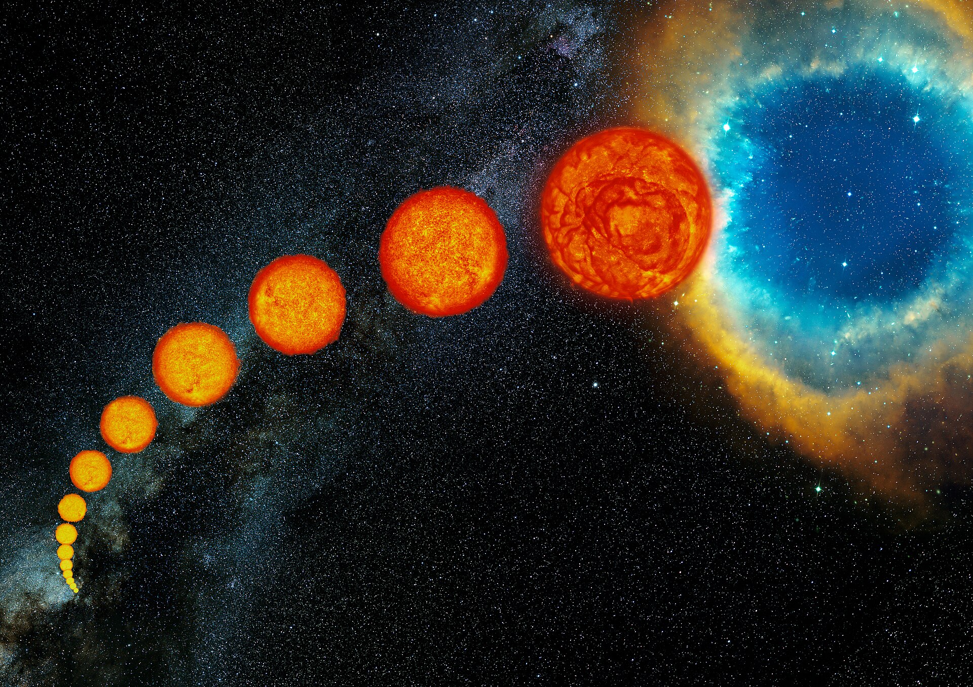
Cooler but larger called red giants.
Our sun is a G2 and is on the main sequence.
4.2.2 Morgan-Keenan Luminosity Classes
Found that there are subtle difference in the strengths of spectral lines for stars of similar temperatures and different luminosities.
Given luminosity class by Roman numerals.
Supergiants have Roman Numeral “I”
Main sequence have Roman numeral “V”
White dwarfs are not classified by this system and are given class “D”
Using this system, distance to star can be found
Feb 12 (Exam I)#
Exam I#
Feb 14#
Stellar Atmospheres Part I#
5.1.1. The Specific and Mean Intensities
Specific Intensity \(I_λ\), function of time, function of cone volume (solid angle, or Steradian)
Solid angle in spherical coordinates, steradian is what \(dΩ\) represents in formulae
Dividing by \(r\) to normalize that volume into a 2D angle but in a 3D space (normalizing radius \(r\) really just is like having longitude and latitude but with a constant radius of the Earth \(R_E\), so you are normalizing out that dimension)
Intensity of radiation:
Spectral/monochromatic intensity: Wien’s law, most intense wavelength is based off of blackbody temp.
Mean intensity:
Considering single ray of light (like a vector arrow), but with \(I_λ\) specific intensity we are talking about a bundle of light rays (cone) and thus the rays (plural) varies in direction
When solving for mean intensity, we are integrating because it is like mean value theorem in calculus, so it’s natural we integrate
5.1.2. The Specific Energy Density
Consider light entering a cylinder with reflective walls, bounces, then exits
Light enters at wavelength range between \(λ\) and \(dλ\)
We are still integrating over the volume of the cylinder to normalize like we did with the mean value theorem of calculus
Energy inside that cylinder:
Specific energy density:
Specific energy density for blackbody radiation:
Total energy density found by integrating over volume:
Total energy density is therefore:
Radiation constant: \(4\sigma/c = 7.565767 \times 10^{-16}\;{\rm J/m^3/K^4}\)
5.1.3. The Specific Radiative Flux
Specific radiative flux:
Talking about radiative disk, radiation that is a circle, but because we have a circular telescope we get rings which are called the airy rings
5.1.4. Radiation Pressure
Most things in solar system affected by pressure due to radiation are low mass dust or some material relaly big like a solar sail which is affected by radiation pressure with large SA
We divide over SA of sphere so leading factor of 2 when dealing with an isotropic radiation field gets divided out
Volume over all solid angles is simply a unit sphere (\(4\pi/3\))
All of this is essentially describing the radiation field from star and with geometry/solid angle/steradian
Blackbody radiation pressure is one-third of the energy density
5.2. Stellar Opacity
Star’s not exactly blackbodies, star’s photosphere devitaes from exact stefan boltzmann law
The color temperature is obtained by fitting the Planck function to the shape of a star’s continuous spectrum.
The kinetic temperature is contained in the Maxwell-Boltzmann distribution, which describes the velocity distribution of gas particles.
The ionization temperature is defined by the Saha equation, which measures the ratio of atoms that are ionized (missing electrons).
The excitation temperature is defined by the Boltzmann equation, which measures the ratio of atoms between two quantum states.
5.2.1. Temperature and Local Thermodynamic Equilibrium
Effective temperature talks about where you are talking about in the star, while remaining temperatures deal with conditions of gas in assumed “ideal box”
Thermodynamic equilibrium, not net flow of energy
Temperature scale height \(H_T\) which is related to average temperature divided by how temperature changes with height in the sun (going through thick slab of sun how does the temperature change)
Temperature scale height exercise 5.1 with computational result
Is the Sun’s photosphere in LTE? Important quesiton, need to find mean free path of particles and phtootons, we take density of photosphere, assume neutral hydrogen atoms in the ground state (good assumption for photosphere because temperature of photosphere not hot enough for atoms to get ionized)
There is also an example of a mean free path exercise 5.2
Mean free path:
Larger result for mean free path because the number of hydrogen atoms is A LOT so “this will greatly increase the cross secitonal area” of likely collisions
Feb 19#
Stellar Atmospheres Part II#
5.2.2. The Definition of Opacity
Any process that removes photons from a beam of light is collectively termed absorption, which includes the scattering of photons (i.e., Compton scattering)
Opacity Equation: Describes the change in intensity I of light through a gas, dependent on intensity \(I_0\) , distance traveled d , and gas density \( \rho \).
Absorption Coefficient κ: Determines opacity, measured in area per unit mass \(\text{m}^2/\text{kg} \), influenced by gas composition, density, and temperature.
Characteristic Length ℓ: Describes how far a photon travels before intensity declines, calculated using the opacity and gas density.
The change in intensity \(dI_\lambda\) of a photon as it travels through a gas is proportional to its intensity \(I_\lambda\), the distance traveled \(ds\), and the density of the gas \(\rho\) through the relation,
The quantity \(\kappa_\lambda\) is called the wavelength-dependent absorption coefficient (or opacity).
5.2.3. Optical Depth
Relation to Intensity: Optical depth affects intensity decline exponentially as light travels through a medium.
Optical Depth Variations: Dependent on material’s properties, density, and wavelength.
Implications: Optical depth impacts radiative flux through a medium.
Mean Free Path : Distance a photon travels before scattering, dependent on wavelength.
The mean free path is dependent on the photon wavelength \(\lambda\). It is convenient to define an optical depth \(\tau_\lambda\) as
where \(s\) is the distance measured along the photon’s direction of motion (i.e., looking back along the path traveled by the photon).
The difference in optical depth \(\Delta \tau_\lambda\) can be determined as the difference between the final (\(\tau_{\lambda,f}\)) and initial (\(\tau_{\lambda,o}\)) optical depths, or the integral along the photon’s path as
The optical depth can be related to the intensity where there is a decline in the intensity given by
The maximum optical depth is typically \(\tau_\lambda \approx 1\), where deeper layers are completely obscured. In some situations, setting \(\tau_\lambda = 0\) occurs inside the star instead of at the surface.
If \(\tau_\lambda \gg 1\), then the gas is optically thick.
If \(\tau_\lambda \ll 1\), then the gas is optically thin.
The intensity of the light before entering the atmosphere is \(I_{\lambda,o}\) and \(I_\lambda\) once it reaches the telescope.The light enters the atmosphere at some angle \(\theta\), where \(ds = -dz/\cos \theta = -\sec \theta dz\).
where \(\tau_{\lambda,o}\) refers to the optical depth of a vertically traveling photon ($\theta = 0). The intensity of the light at the telescope is
5.2.4. General Sources of Opacity
Opacity Sources: Absorption and scattering processes remove photons, contributing to opacity.
Primary Sources: Bound-bound transitions, bound-free absorption, free-free absorption, and electron scattering.
Influence: Opacity depends on chemical composition and particle interactions.
Gaunt Factors: Quantum-mechanical corrections influencing opacity.
Kramers Opacity Law: Empirical model describing opacity’s temperature and density dependence.
The opacity of a material depends on the chemical composition and how photons interact with the particles (atoms, ions, and free electrons) within the material.
If a photon passes within \(\sigma_\lambda\) (i.e., the particles’s cross-sectional area) of the particle, then the phone can be either: scattered or absorbed.
In an absorption process, the photon ceases to exist and its energy is incorporated into the thermal energy of the gas.
In a scattering process, the photon just continues along in a different direction.
There are four primary sources of opacity available for removing photons from our observations of a star.
Bound-bound transitions are electron transitions from one orbital to another (i.e., excitation and de-excitation).
Bound-free absorption, or photoionization, occurs when an incoming photon has enough energy to free, or ionize, an atom.
Free-free absorption is a scattering process that occurs when the speed of a free electron increases (or decreases) after a nearby ion absorbs (or emits) a photon, respectively.
Electron scattering is as you would expect where a photon is scatter (not absorbed) by a free electron through the process of Thomson scattering.
The cross section for Thomson scattering \(\sigma_T\) has the same value (independent of wavelength)
- \[ \sigma_T = \frac{1}{6\pi\epsilon_o^2}\left( \frac{e^2}{m_e c^2}\right) = 6.65 \times 10^{-29}\:{\rm m^2}.\]
A photon can also be scattered by loosely bound electrons. Compton scattering occurs when the photon’s wavelength is much smaller than the atom or Rayleigh scattering if the wavelength is much larger.
The opacity of stellar material suddenly increases at wavelengths \(\lambda \leq 364.7\:{\rm nm}\) and the measured radiative flux of the star suddenly decreases. This abrupt drop in the continuous spectrum is the Balmer jump and is evident in the Sun’s spectrum.
\(H^-\) ion photoionization occurs in the atmospheres of stars later than F0 and is the primary source of continuum opacity, \(\kappa_{H^-}\). At longer wavelengths \(H^-\) contributes to opacity through free-free absorption (i.e., more free electrons become available through photoionization).
Rayleigh scattering is important in planetary atmospheres and is responsible for Earth’s blue sky.
5.2.5. The Rosseland Mean opacity
Mean Opacity Definition: Averaged opacity over all wavelengths, reflecting composition and density.
Rosseland Mean: Weighted average opacity considering blackbody spectrum variation with temperature.
Dependence on Parameters: Density, temperature, and composition influence mean opacity.
Quantum Effects: Gaunt factors and guillotine factor contribute to opacity calculations.
The most commonly used scheme to compute a wavelength-independent opacity is the Rosseland mean opacity or the Rosseland mean. The Rosseland mean incorporates a weighting function that depends on how fast the blackbody spectrum varies with temperature, which is defined as
Approximation formulae have been developed for the average bound-free and free-free opacities:
which depends on the density \(\rho\), temperature \(T\), the hydrogen mass fraction \(X\).
The mass fractions are formally defined as
such that \(X+Y+Z = 1\).
5.3 Radiative Transfer
Equilibrium Conditions: Stellar atmospheres maintain balance in energy absorption and emission.
Emission Processes: Includes scattering and true emission through electron transitions.
Effect on Photon Flow: Absorption and emission processes hinder photon flow, leading to randomized paths.
Describes stellar atmospheres are in equilibrium or a steady state. This means that the mechanisms involved in absorbing and emitting energy must be in balance throughout the star so that no change in total energy occurs within any layer of the interior.
5.3.1. Photon Emission Processes
Emission is defined as any process that adds photons to a beam of light, which includes the scattering photons into the beam and the true emission of photons through electron transitions.
5.3.2. The Randowm Walk
As the photons move through the stellar material, they follow a random walk (i.e., a haphazard path). Between each atomic encounter, the photon travels a path \({\bf \ell}\) (the mean free path), which can be summed over a large number \(N\) directed steps to produce a net vector displacement d:
Through a random walk, the transport of energy through a star by radiation alone can be extremely inefficient. The optical depth is roughly the number of mean free paths \(\ell\) that a photon must travel to get to the surface, which implies that \(d = \tau_\lambda \ell = \ell\sqrt{N}\). The average number of steps needed to travel to a distance \(d\) is
for \(\tau_\lambda \gg 1\). When \(\tau_\lambda \approx 1\), a photon can potentially escape from that depth, but a more carful analysis shows the average depth of the atmosphere from which photons can escape is \(\tau_\lambda = 2/3\).
5.3.3. Limb Darkening
An observer looking at the Sun’s disk sees the brightest (hottest) portion near the center due to optical depth (\(\tau_\lambda = 2/3\)), observations near the edge (or limb) of the Sun appear darker (cooler). At the limb, the penetration depth only reaches the uppermost (cooler) layers of the atmosphere and we will see a lower temperature compared to the center of the disk. This effect is called limb darkening, where astronomers have to account for it in transit photometry
5.3.4. The Radiation Pressure Gradient
In addition to the photon’s journey, there is a pressure that build’s within the Sun’s atmosphere due to collisions. The pressure outside is lower than the pressure inside the room, which can be expressed as a pressure differential using Bernoulli’s principle.
The extent of the difference is not uniform, where the pressure decreases with stellar radius (i.e., as you get closer to the surface). But it is enough to create a light movement of photons toward the surface that described by
The transfer of radiation as a flow with photons drifting toward the surface is a better description than a “beam” that propagate radially outward.
Feb 21#
Stellar Atmospheres Part III#
5.4 The Transfer Equation#
5.4.1 The Emission Coefficient#
Interested in the net flow of energy, not the specific path. The intensity can be increased through emission. This change is \( dI_{\lambda} \) is proprtional to the the distance \( ds \) and the density of the gas \( \rho \).
here, \( j_{\lambda} \) is the emission coefficient.
The specific intensity \( I_{\lambda} \), changes as the photons are added. Combining the equations of absoption and emission gives the general result;
5.4.2 The Source Function and the Transfer Equation#
To determine the ratio of emission to absorption ( \( j_{\lambda} / \kappa_{\lambda} \) ), we cal this the source function \( S_{\lambda} \) and looks like;
If \( I_{\lambda} > S_{\lambda} \) then the intensity decreases with distance. If \( I_{\lambda} < S_{\lambda} \), then the intensity increases with distance.
5.4.3 The Special Case of Blackbody Radiation#
For a blackbody, the intensity is equal to the Planck function ( \( I_{\lambda} = B_{\lambda} = S_{\lambda} \) ) [for something in thermodynamic equalibrium which stars are not in!]
Applying the transfer equation
5.4.4 The Assumption of a Plane-Parallel Atmosphere#
Rewrite the transfer equation as a function of optical depth;
Because the atmosphere is not a plane (it curves) we assume a plane-parallel slab of the atmosphere and get the equation for vertical optical depth;
A gray atmosphere is an atmosphere that has little to no wavelength dependence. The transfer equation for a gray atmosphere is;
5.4.5 The Eddington Approximation#
When looking at a star, we see down to a vertical optical depth of , averaged over the disk of the star.
5.5 The Profiles of Spectral Lines#
5.5.1 Equivalent Widths#
Absorption spectral lines are identified on graphs of the radiant flux \( F_{\lambda} \) as a function of the wavelength \( \lambda \).
Full width half maximum (think inverse bell curve and take the half of the lowest point on either side and make a rectangle to connect these two with the max point of the inverse bell curve.)
5.5.2 Proccess that Broaden Spectral Lines#
Natural Broadening: the spectral lines cannot be sharp even for motionless, isolated atoms due to Heisenberg’s uncertainty principle.
where \( \Delta t_0 \text{ and } \Delta t_f \) is the lifetime of the electron in the initial state and final state respectively.
Doppler Broadening: The wavelengths of the absorbed or emitted light are Doppler-shifted nonrelativistically according to \( \Delta \lambda / \lambda = +- | v_r | / c \). The width of a Doppler broadened spectral line should be;
Pressure (and Collisional) Broadening: the atomic orbitals are perturbed by a collision with a neutral atom or a close encounter with the electric field of an ion. Statistical is pressure, individual collisions is collisional. To determin collisional pressue, we need to determine the average time between collisions \( \Delta t_0 \), and the mean free path \( \ell \). These are related through the following equation;
where \( m \) is the atom mass, \( \sigma \) is the collisional cross-section, and \( n \) is the number of atoms. From the collisional pressure, we can determine the spectral line width broadening to be;
Spectral line width is proportional to \( n \).
5.5.3 The Voigt Profile#
The total line profile is called the Voigt profile and is due to the contributions of the Doppler and the damping things. Doppler contributes more for the center wavelengths whereas the damping profile is more towards the wings of the curve.
The goal is to determine \( N_0 \), which is the coloumn density.
5.5.4 The Curve of Growth#
Helps determine the value of \( N_a \) (the number of atoms that have electrons in the proper orbital for absorbtion) and the abundance of elements in stellar atmospheres. The width W varies with \( N_a \) and therefore a log curve can be used to estimate the change in both quantities. Using the curve of growth, and a determined width, we can determine the number of absorbing atoms.
Feb 26#
The Sun Part I#
6.1.1. The Evolutionary History of the Sun#
Our Sun is classified as a typical main-sequence star of spectral class G2, which contains mostly hydrogen \((X=0.74)\), some helium \((Y=0.24)\), and a little metal \((Z=0.02)\) by mass.
Since becoming a main-sequence star, the Sun’s luminosity has increased by nearly 48% and its radius has increased by 15%, which lead to an increase a 2.7% increase in its effective temperature.
6.1.2. The Present-Day Interior Structure of the Sun#
Using the current age of the Sun, a solar model must reproduce the current values of the central temperature, pressure, density, and composition.
solar model: A mathematical treatment of the Sun as a spherical ball of gas. This model is used to predict the internal observables like neutrino fluxes and oscillation frequencies and consequently to validate its assumptions for its generalization to other stars
nucleosynthesis: Is the creation of new atomic nuclei, the centers of atoms that are made up of protons and neutrons
The Sun’s primary energy production comes from the proton-proton (pp) chain, where, or tritium is an intermediate species in the reaction sequence.
Tritium is relatively more abundant at the top of the hydrogen-burning region where the temperature is lower. At greater depths, the higher temperatures the destroy the tritium more often than it is created, resulting in a overall decrease in abundance.
Mass conservation equation:
\[\frac{dM_r}{dr}=4\pi r^2 \rho →dM_r=4\pi r^2 \rho \space dr=\rho \space dV,\]which indicates how the mass within a certain radius interval increases because the volume of a spherical shell increases with a fixed choice of \(dr\).
The energy generated in the interior has to be transported outwards, where a criterion for the onset of convection is that the temperature gradient becomes superadiabatic,
\[\left|\frac{dT}{dr}\right|_{\text{actual}}> \left|\frac{dT}{dr}\right|_{\text{adiabatic}}\]where actual and adiabatic refer to the temperature gradients. For an ideal monatomic gas, this conditions becomes, $\(\frac{d \ln P}{d \ln T}< 2.5\)$
6.1.3. The Solar Neutrino Problem: A Detective Story Solved#
Neutrino flux: A measurement of the intensity of such a neutrino stream.
The neutrino has a very low cross section for interaction with other matter, which makes it difficult to detect. Neutrinos penetrate where other particles cannot.
The Mikheyev-Smirnov-Wolfenstein (or MSW) effect involves transformation of neutrinos between the three types \((\nu_{\mu}, \nu_{\tau}, and \nu_e)\).
Super-Kamiokande was used to detect atmospheric neutrinos produced in Earth’s upper atmosphere.
Super-Kamiokande determined that the number of \(\nu_\mu\) traveling upward was significantly reduced compared to those traveling downward, where the difference in numbers is in excellent agreement with the theory of neutrino mixing.
For neutrino mixing to occur, the neutrino could not be a massless particle and the experiment confirmed this as well.
Cosmic rays are capable of producing only electron and muon neutrinos.
6.2. The Solar Atmosphere#
6.2.1. The Photosphere#
Optical photons appear to originate from an outer layer of the Sun called the photosphere. The base of the photosphere is somewhat arbitrary since photons because some photons originate from deep within the Sun \((\tau_{\lambda}\gg 1)\)
The optical depth from a given layer \(\tau_{\lambda}\) can be estimated from an estimate of the fraction of photons that we receive from that layer (i.e., \(\tau_{\lambda}=- \ln \left(\frac{I_{\lambda}}{I_{\lambda, o}}\right)\)).
On average, the solar flus is emitted from and optical depth \(\tau=2/3\) (the Eddington approximation), which leads to defining the effective temperature (for Wien’s law) at this depth.
Using the Saha equation, we can determine the ratio of \(H^-\) ions to the neutral hydrogen atoms.
From Kirchhoff’s laws, the absorption lines are produced when there is a cooler gas between the observer and the bulk of the hot source (i.e., continuum-forming region). In reality, the Fraunhofer lines are formed in the same layers where \(H^-\) ions produce the continuum.
6.2.1.1. Solar Granulation & Differential Rotation#
This structure is called granulation and represents the top portion of a convection zone protruding into the photosphere’s base.
Granulation causes wiggles to appear in the absorption lines due to small Doppler shifts (400 m/s) from the convection cycle.
The brighter regions produce blueshifts (i.e., rising hot material) in the absorption lines while the darker regions are caused by redshifts (i.e., sinking cool material).
The lifetime of a granule is defined as the amount of time for a parcel to rise and fall the distance of one mixing length.
The absorption lines are used to measure the rotation rate of the Sun, where measurements are taken from the equator and then outward with increasing latitude.
Tachocline: is the transition region of stars of more than 0.3 solar masses, between the radiative interior and the differentially rotating outer convective zone.
6.2.2. The Chromosphere#
Above the photosphere lies a portion of the Sun’s atmosphere called the chromosphere that is only about 0.01% (or a factor of \(10^{-4}\)) of the photosphere’s intensity and extends upward for approximately 1600 km or 2100 km above \(\tau_{500}=1.\)
Certain Fraunhofer lines appear as absorption lines in the visible and near-UV, where others begin to appear as emission lines at shorter (or much longer) wavelengths.
Kirchhoff’s laws suggest that a hot, low-density gas must be responsible for the emission lines. The emission cannot occur deep within the Sun’s interior because the Sun is optically thick and so the area of emission line production occurs elsewhere.
Emission lines (in the visible range) are observable near the limb of the Sun for a few seconds when the bright solar disk is occulted during a total eclipse and is known as a flash spectrum.
On scales of 30,000 km, the continued effects of the convection zone are seen as supergranulation. Similar to granules, Doppler studies reveal the rising and sinking of gas at 400 km/s.
Spicules, or vertical filaments of gas, are present that extend upward for 10,000 km and each spicule has a lifetime of only 15 minutes. As a result the speed of particles in spicules move upwards at approximately 15 km/s, as shown through Doppler studies.
6.2.3. The Transition Region#
The temperature rises rapidly within approximately 100 km above the chromosphere and reach \(> 10^5\) K before \(dT/dr\) begins to flatten. The temperature still increases, but more slowly until eventually exceeding \(10^6\) K. Selective observations in the UV and extreme-UV reveal this transition region.
6.2.4. The Corona#
During a total solar eclipse, a faint corona appears around the Sun at totality. The corona lies above the transition region, extends out into space without a well-defined outer boundary, and is very faint (about \(10^6\) times less intense) compared to the photosphere.
The corona is essentially transparent to most EM radiation (except long radio wavelengths) and is not in LTE. For gases that are not in LTE, a unique temperature is not strictly definable.
The low number densities in the corona allow forbidden transitions to occur from atomic energy levels that are metastable (or temporarily stable).
The corona is a source of radio emission, where some of this emission arises from free-free transitions as electrons pass near ions.
Encounters in a higher density region (i.e., nearer to the Sun) result in shorter wavelength photons, where encounters in the chromosphere and lower corona (with much lower density) emit longer wavelength radiation \((1-20\) cm).
X-ray emissions from the photosphere are also rare, where the blackbody continuum decreases more rapidly (i.e., Wien approximation). Thus, any X-ray emission from the corona overwhelms the contribution from the photosphere due to its high temperature and low opacity at X-ray wavelengths.
The corona contains a high degree of ionization for all the elements present, where the neutral atoms undergo a large number of transitions. Each element is capable of producing ans extensive emission spectrum.
6.2.4.1. Coronal Holes and the Solar Wind#
Observations show that X-ray emission is non-uniform, where active (bright and hot) regions exist along with the coronal holes (darker and cooler regions).
A weaker X-ray emission coming from the coronal holes is characteristic of the lower density and temperature of the region.
The existence of coronal holes is tied to the Sun’s magnetic field and the generation of a fast solar wind.
Coronal holes correspond to regions where the magnetic field lines are open, while the X-ray bright regions are associated with closed field lines. Closed field lines form loops that return to the Sun, while open field lines extend out to great distances.
For charged particles moving in an external magnetic field, the Lorentz force equation applies \(F=q(E+V \times B),\) which describes the force \(F\) exerted on a charged particle with a velocity \(v\) in an electric field \(E\) and magnetic field \(B\)
Feb 28#
The Sun Part II#
Mar 4#
The Interiors of Stars Part I#
Teaching Presentations#
Mar 6#
The Interiors of Stars Part II#
Teaching Presentations#
Mar 11 & 13 (Spring Break)#
No Class#
Mar 18#
The Interiors of Stars Part III#
Teaching Presentations#
Mar 20#
The Interiors of Stars Part IV#
Teaching Presentations#
7.3.7
PPI Chain: first fusion process chain with two hydrogen-1
One of the protons undergoes beta decay to change to a neuton, neutrino, and positron which then combines witht he other to become deuterium. $\( _1^1H + _1^1H \rightarrow _1^2H+e^++\nu_e\)$
Deuterium and proton combine to create He-3 and photon. $\( ^2_1H+^1_1H \rightarrow ^3_2He+\gamma\)$
Finally two He-3 atoms combine to create He-4 and 2 protons $\( ^3_2He +^3_2He \rightarrow ^4_2He+2 ^1_1H\)$
PPII Chain: Second part of intial fusion reaction using the He-3 and He-4 and a proton to create 2 He-4 $\( ^3_2He+^4_2He\rightarrow ^7_4Be+\gamma\)\( \)\(^7_4Be +e^- \rightarrow ^7_3Li +\nu_e\)\( \)\(^7_3Li+^1_1H\rightarrow2 ^4_2He\)$
PP III: Combination of the Be-7 from PPII of a proton instead of an electron to create 2 more He-4 $\(^7_4Be +^1_1H\rightarrow ^8_5B+\gamma\)\( \)\(^8_5B\rightarrow^8_4Be+e^++\nu _e\)\( \)\(^8_4Be\rightarrow 2^4_2He\)$
7.3.8
CNO cycle uses heavy nuclei as catalyst
CNO I produces carbon-12 and Helium-4
CNO II only occurs 0.04% of the time and produces Nitrogen-14 and Helium-4
7.3.9
Triple alpha process produces Carbon-12 out of Helium-4 $\( ^4_2He +^4_2He ⇌ ^8_4Be\)\( \)\( ^8_4Be +^4_2He \rightarrow ^{12}_6C+\gamma\)$
7.3.10 Carbon and Oxygen Burning
Carbon captures alpha particles to create oxygen
Helium outside carbon core produce oxygen which then combine to create neon
T = 60 million K
two carbon-12 can produce either Oxygen-16 and 2 Helium-4, Neon-20 and Helium-4, Sodium-23 and proton, Magnesium-23 and Neutron, or Magneisum-24 and gamma
7.3.11 Binding energy per nucleon $\( E_b = [Zm_p+(A-z)m_n-m_nucleus]c^2\)$
The binding energy per nucleon increases until iron-56, where it begins to decrease
Hydrogen-1, Helium-4, and Oxygen-16 are most stable (and abundant) nuclei.
Iron-56 is most stable with highest binding energy. Stars build up nuclei starting at lighter elements up to iron. All others are made during supernovae.
Past Iron peak, more energy needed and thus fission begins.
7.4 Energy Transport and Thermodynamics#
7.4.1 Three Energy Transport Systems#
Radiation: energy from nuclear reaction carried to the surface through photons. (middle efficient)
Convection: cooler elements fall inward, hotter elements are carried outwards (most efficient)
Conduction: transport via collisions between particles (least efficient so less significant.)
7.4.2 The Radiative Temperature Gradient#
The radiation presure gradient equation;
where \(r\) is the distance from the center (radius). Adding the equation for \(F_{rad} = \frac{L}{4 \pi r^2}\), we have;
7.4.3 The Pressure Scale Height#
If the gradient becomes too steep, convection becomes more efficient (hot air moving up cold air moving down). A characteristic length for convection is the pressure scale hieght \(H_p\) is defined as;
assuming \(H_p\) is constant we solve for the pressure with radius as;
If \(r = H_p\) then \(P=P-0/e\) and then \(H_p\) is the distance over which the gas pressure decreases by a factor of \(e\). We can write the pressure gradient in terms of the local acceleration of gravity %g = \frac{GM_r}{r^2}. Sub this in and we get;
7.4.4 Internal Energy and the First law of Thermo
First law relating to energy transfer states $\(dU = \delta Q-\delta W\)$ which describes change in internal energy (U) is modified by difference in Work (W) done and heat added (Q).
U is a state function meanging it desrcibes current condition of the gas. dU is thus independent of the process. Heat added and work done depends on the order of processes that are carried out.
Mar 25#
The Interiors of Stars Part V#
Teaching Presentations#
7.4.4 Internal energy and the first law of Thermodynamics
A basic understanding of convective Heat transport begins with thermodynamics $\(dU = \delta Q - \delta W\)$
This equation describes how internal energy of a mass element \(dU\) is modified by the difference of the work done \(\delta W\) by that element from the heat added \(\delta Q\) to that element.
State function (value represents the present condiitions of the gas)
The internal energy (U) is a function of the gas compostion and temperature. In this case, the internal energy is jsut the kinetic energy per unit mass.
In an ideal monoatomic gas with on ionization
7.4.5 Specific Heats
Specfic heat (\(C\))
the amount of heat \(\delta Q\) required to raise the temperature of a unit mass of a material by a unit temperature $\( C_p \equiv \frac{\partial Q}{\partial T}\bigg\rvert_P \qquad \text{and} \qquad C_V \equiv \frac{\partial Q}{\partial T}\bigg\rvert_V, \)$Consider the amount of work per unit mass done by the gas on its surrounds, suppose that a cylinder of a cross-sectional area is filled with a gas of mass m and pressure. $\(\delta W = \frac{F}{m}dr = \frac{PA}{m}dr = PdV,\)\( \)\(dU = \delta Q - PdV.\)$
for a monatomic gas, γ =5/3 a. If ionization occur , the temperature of the gas will not rise as rapidly becasue some of the heat goes into ionizing athe atoms instead of increasing the average kinetic energy of the particles.
7.4.6. The adiabatic Gas Law
Since the change in internal energy is independent of the process involved there is a special proccess called the Adiabatic process where no heat flow into or out of a mass element ( no heat exchange)
adiabatic gas law is $\(PV^{γ}=Κ\)$
Using the ideal gas law, a second adiabatic relation is found,
7.4.7. The Adiabatic Sound Speed
The sound speed \(v_s\) through the material is related to the compressibility of the gas and its inertia.
The bulk Modulus \(B\) of the gas describes how much the volume of the gas will change with pressure and is defined as
aadiabatic sound speed
7.4.8. The Adiabatic Temperature Gradient
Convecitons bubbles are parcels of hot gas that rise and expand adiabatically. After travleling a certain distance the parcel gives up excess heat as it loses its identity and dissolved into the surrounding gas.
Treating the convection bubble as an ideal gas requires knowledge of how it is modified with changing stellar radius. ( differentiation of ideal gas law)
Upon differentiations with repsect to r, we obtain $\( \frac{dP}{dr} = \frac{1}{\gamma}\frac{dP}{dr} + \frac{P}{T}\frac{dT}{dr}. \)$
adiabatic temperature gradient is defined as
This equation can be written im simpler forms using the local acceration of gravity g
This result describes how the temeprature of the gas inside the bubble changes as the bubble rises and expands adiabatically.If the star’s actual temperature gradient is steeper than the adiabatic temperature gradient, or
the temperature is Superadiabatic - stars actual temperature gradient is steeper than the adiabatic temperature gradient
if the deep inerior of a star is just slightly superadiabatic, then it may be possibel to carry nearly all the luminosity by convection.
often the case that radiaiton of convections dominates the energy transport in the deep interior,but near the sufface both radiation and conveciton carry significant amounts of energy simultaneously.
7.4.9. A Criterion of Stellar Convection
Questions regarding when convections occurs
What conditions must be met if convecitons is to dominate over radiation in the deep interior
When will a hot bubble of gas continue to rise rather than sink
To express this condition in terms of temperature gradients, assume that
the gas is initially, very nearly in thermal equilibrium \((T_i^{(b)}\simeq T_i^{(s)}\:\text{and}\:\rho_i^{(b)}\simeq \rho_i^{(s)})\),
the bubble expands adiabatically (i.e., no heat exchange), and
the bubble and surrounding gas pressures are equal at all times \((P_f^{(b)} = P_f^{(s)})\).
For an ideal monatomic gas \(\gamma = 5/3\) and the RHS of Eqn. (7.65) is 2.5. Once \(d\ln P/d\ln T\) is greater than 2.5, then the region is stable against convection. In general, convection will occur when
the stellar opacity is large, implying that an unattainable steep temperature gradient would be necessary for radiative transport,
a region exists where ionization is occurring, causing a large specific heat and low adiabatic temperature gradient, and
the temperature dependence of the nuclear energy generation rate is large, causing a steep radiative flux gradient and a large temperature gradient..
#7.5. Stellar Model Building
7.5.1 A summary of the Equations of Stellar Structure
The basic time-indendent stellar structures equations are summarized as $\( \boxed{\begin{align*} \frac{dP}{dr} &= -\frac{GM_r \rho}{r^2} &\\ \frac{dM_r}{dr} &= 4\pi r^2 \, \rho &\\ \frac{dL_r}{dr} &= 4\pi r^2 \, \rho\,\epsilon &\\ \frac{dT}{dr} &= -\frac{3}{4ac}\frac{\overline{\kappa}\rho}{T^3}\frac{L_r}{4\pi r^2} & \text{(radiation)} \\ &= -\left(1 - \frac{1}{\gamma} \right)\frac{\mu m_H}{k}\frac{GM_r}{r^2} & \text{(adiabatic convection)} \end{align*}}\)$
The convective (adiabatic) temperature gradient can be applied when
7.5.2 Entropy
gravitational energy generation rate can be expressed in terms of the change in entropy per unit mass by
if the star is collapsing, \(ϵ_\text{gravity}\) is positive \(+\) otherwise it will be negative. As the star contracts, its entropy decrease. A star is not a closed system, where its entropy may decrease locally while the entropy of the universe due to radiaiton and stellar wind.
7.5.3 The Constitutive Relations
Constitutive relations - required conditions are the equations of the state.
rest(tba)
7.5.4. Boundary Conditions(TBA)
7.5.5. The Vogt-Russell Theorem
A summary of how everything in a stars system is connected
The pressure gradient depends on the interior mass and densisty
the radiative temperature gradient depends on the local temperature, density, opacity, and interior lumnosity
the Luminosity gradient functions depends on the density and energy generation rate
The Vogt-Russell Theorem The mass and the composition structure throughout a star uniquely determine its radius, luminosity, and internal structure, as well as its subsequent evolution.
The dependence of a star’s mass and composition evolution is a consequence of the change in composition due to nuclear burning (i.e., fusion). There are other factors (e.g., magnetic fields and rotation) that influence stellar interiors, but these are assumed to have little effect in most stars.
7.5.6. Numerical Modeling of the Stellar Structure Equations
polytropes - a special family of approximate solutions to the stelalr structure 3
the system of differential equations for the stellar strucutre cannot be solved analytically for all cases. making it neccessary to evalute the DE numerically by approximating the equations by difference equations. then the star is modeled as a set of spherically symmetric shells and the integration is carried out starting from some initial radius in finite steps.
An example of this can be found for pressure \(Ρ\)
7.5.7. Polytropic Models and the Lane-Emden Equation (TBA)
Under very special situations, it is possible to find analtic solutions to a subset of the stellar structure equations. The famous equation that helps us describe analytical stellar models is the Lane-Emden equation.
If a simple realtionshpi existed bewteen pressure and densisty, then the mechanical equations for stellar structure could be solved simultanesouly
treats star asa fluid( very complicated math)
#7.6. The Main Sequence
7.6.1. The Eddington Luminosity limit
the stability of very massive stars is directly affected thier luminosity, if the temperature is high and gas density is low, then it is possible for radiation pressure to dominate over the gas pressure. When this occurs the outer portions of very massie stars, the outer layers disperse due to the intense stellar wind.
The pressure gradient near the stellar surface is
Eddington Limit
the maximum radiative luminosity, aka a maximum value for a star to remain in hydrostatic equilibrium.
\[ L_{\rm Ed} = \frac{4\pi r^2 c}{\overline{\kappa}}g = \frac{4\pi G c}{\overline{\kappa}}M_\star. \]It is possible to deteremien the Eddington limit of stars at the end of the main sequence, since most of their effective temperatures is ≈50,000K,
\[ L_{\rm Ed} = \frac{4\pi G c}{\overline{\kappa}_{es}}{M_\odot} = \frac{200\pi Gc}{(1+X)}{M_\odot} = 1.5\times 10^{31}\:{\rm W},\]or
7.6.2. Variations of Main-Sequence Stellar Parameters with Mass
From theoretical models computed in the mass range of hydrogen burning, it is possible to obtain a numerical \(M-L\) relationship that agrees well with the observational \(M-L\) relationship. Stars undergoing hydrogen burning in the cores lie along the observational main sequence.
This is approximately in the range of \(5\times 10^{-4}\:L_\odot\) to \(1 \times 10^6\:L_\odot\)
Mar 27 (Exam II take-home)#
The Interstellar Medium and Star Formation Part I#
Apr 1#
The Interstellar Medium and Star Formation Part II#
8.2.4. Additional Physical Processes in Protostellar Star Formation
Zeeman measurements of various molecular clouds indicate the presence of magnetic fields with strengths from \(1 - 100 nT\).
The term “froze-in” refers to Alfven’s theorem, which states that “in a fluid with infinite electric conductivity, the magnetic field is frozen into the fluid and has to move along with it.”
The virial theorem was invoked during the derivation of the Jean’s criterion as a balance between the gravitational potential energy and the cloud’s internal (thermal) kinetic energy. The magnetic field energy was ignored, where including the effects of the magnetic field produces a critical mass of
If the magnetic field strength \(B\) is expressed in \({\rm nT}\) and the cloud radius \(R\) in units of \({\rm pc}\), then \(M_B\) can be written as
8.2.5. Ambipolar Diffusion
Another possibility for triggering the collapse of a dense core is through change of state. If a core that was originally subcritical became supercritical , then collapse could ensue. This could have in a couple of ways:
A group of subcritical clouds could combine to form a supercritical cloud, or
the magnetic field could be rearranged so that the field strength is lessened in a portion of the cloud.
To determine the relative impact of ambipolar diffusion, we need to estimate the characteristic timescale. By knowing the drift velocty, it can be shown that
8.2.6. Numerical Simulations of Protostellar Evolution
Consider a spherical cloud of approximately \(1\,M_\odot\) and solar compositions that is supercritical. Initially, the early stages of free-fall collapse are nearly isothermal because the absorption by the dust is relatively inefficient (i.e., photons have a significant mean free path). The central region (radius of ~\(5\,{AU}\)) is nearly in hydrostatic equilibrium and this central object is then referred to as a protostar.
An observable consequence of the cloud becoming optically thick is that the gravitational potential energy released during the collapse is converted into heat and then radiated away in the IR. The curves on the H-R diagram depict the life histories of the simulated clouds are known as evolutionary tracks. As the collapse continues to accelerate, the luminosity of the protostar increases along with its effective temperature.
The hydrostatic core slowly increases as more overlying material continues to fall onto it. After the core radius decreases to ~\(1.3\,R_\odot\), hydrostatic equilibrium is re-established. The core mass is still accreting gas, where the final mass will be larger.
8.3. Pre-Main-Sequence Evolution
8.3.1. The Hayashi Track
As the protostar collapse slows, its luminosity decreases while its effective temperature increases slightly and is known as the Hayashi track (i.e. a downward turn at the end of the evolutionary tracks). The Hayashi track represents a boundary between “allowed” and “forbidden” hydrostatic stellar models.
8.3.2. Classical Calculations of Pre-Main-Sequence Evolution
Consider the pre-main-sequence evolution of a 1 \(M_\odot\) star, beginning on the Hayashi track. With the high \({\rm H^-}\) opacity near the surface, the star is completely convective for the first 1 Myr, where deuterium burning also occurs during this early period of the collapse.
As the central temperature continues to rise, the levels of ionization increase but the opacity decreases.
As the radiative core develops, more of the star’s mass is encompassed by the core.
Following the descent along the Hayashi track, the luminosity reaches a minimum and the radiative core allows energy to escape into the convective envelope more readily.
This causes the luminosity to increase again and the effective temperature increases since the star is still shrinking.
The CNO reactions have a high temperature dependence and a temperature gradient is established in the core so that some convection begins to develop there.
When the carbon-12 is exhausted (for the CNO cycle), the core completes its readjustment to nuclear burning, where the remainder of the PP I chain becomes important.
If the protostar mass is \(\lesssim 0.072\,M_\odot\), the core never gets hot enough to generate sufficient energy by nuclear reactions to stabilize the star against gravitational collapse. The stable hydrogen-burning main sequence is never obtained, which explains the lower end of the main sequence.
8.3.3. The Formation of Brown Dwarfs
The objects between \(0.013-0.072\,M_\odot\) are known as brown dwarfs and have spectral types L and T. The first confirmed discovery of a brown dwarf (Gliese 229B) was announced in 1995. Hundreds of brown dwarfs have been detected in near-IR all-sky surveys, such as 2MASS or SDSS.
8.3.4. Massive Star Formation
For massive stars, the central temperature quickly becomes high enough to burn carbon-12 and convert hydrogen into helium-3. This means that these stars leave the Hayashi track at higher luminosities and evolve nearly horizontally across the H-R diagram.
8.3.5. Possible Modifications to the Classical Models
Theoretical evolutionary sequences beginning with smaller initial radii lead to a birth line where protostars become visible, which places an upper limit on the observed luminosities of protostars.
8.3.6. The Zero-Age Main Sequence (ZAMS)
The zero-age main sequence (ZAMS) is known as a diagonal line in the H-R diagram that indicates when stars of various masses reach the main sequence and begin equilibrium hydrogen burning.
8.3.7. The Initial Mass Function (IMF)
The number of stars that form per mass interval per unit volume is strongly mass-dependent, where this functional dependence is known as the initial mass function (IMF). A particular IMF depends on a variety of factors, including the local environment in which a cluster of stars forms.
8.3.8. \({\rm H\,II}\) Regions
The \({\rm H\,II}\) regions are in equilibrium if they have equal rates of ionization and recombination. During recombination, the electron cascades downward and produces a number of lower-energy photons (many will be in the visible). The dominant visible wavelength comes from the \(n=3\) to \(n=2\) transition, or the \({\rm H\alpha}\) line of the Balmer series. Therefore, \({\rm H\,II}\) regions appear to fluoresce in red light.
Emission nebulae are considered to be the most beautiful objects in the night sky, where one particularly famous \({\rm H\,II}\) region is the Orion Nebula (M42). The Orion A complex contains M42, a giant molecular cloud (OMC 1), and a very your star cluster (the Trapezium cluster).
The size of an \({\rm H\,II}\) region can be estimated by considering the equilibrium requirement. The recombination rate can be multiplied by the volume of the \({\rm H\,II}\) region (assumed to be a sphere) and then set equal to the number of ionized photons produced per second. This is expressed as
which solving for the radius produces
and is called the Strömgren radius \(r_S\).
8.3.9. The Effects of Massive Stars on Gas Clouds
After reaching the main sequence, the surrounding gas will ionize, resulting tin the creation of a \({\rm H\,II}\) region inside of a \({\rm H\,I}\) region. Due to the star’s high luminosity, radiation pressure will begin to drive significant mass loss that can disperse the remainder of the cloud. Some famous examples of this occurring are in the Carina Nebula (about 3000 pc from Earth) and in the Eagle Nebula (M16).
8.3.9.1. OB Associations
Groups of stars that are dominated by O and B main-sequence stars are called OB associations, where studies show that they cannot remain gravitationally bound to on another due to their individual kinematic velocities and masses.
8.3.9.2. T Tauri Stars
There is a low-mass pre-main-sequence object that represents a transition from protostars still shrouded in dust and main-sequence stars, which is called a T Tauri star.
T Tauri stars are characterized by unusual spectral features and by large irregular luminosity variations (with timescales on the order of days).
8.3.9.3. FU Orionis Stars
A T Tauri star star can go through a significant increase in its mass accretion rate \((\dot{M} = 10^{-4}\,M_\odot/{\rm yr})\) and luminosity (by four orders of magnitudes or more) that lasts for decades. The firs star to undergo these abrupt changes was FU Orionis, where similar behaving stars are called FU Orionis stars.
8.3.9.5. Herbig-Haro objects
Mass loss during pre-main-sequence evolution can also occur from jets of gas that are ejected in narrow beams in opposite directions. Herbig-Haro objects (HH objects) were discovered in the early 1950s by George Herbig and Guillermo Haro in the vicinity of the Orion nebula and are associated with the jets produced by young protostars (e.g., T Tauri stars).
8.3.10. Young Stars with Circumstellar Disks
Observations have revealed that other young stars also possess circumstellar disks of material, where two well-known examples are Vega and \(\beta\) Pictoris. An IR image of \(\beta\) Pic shows its disk, where observations of \(\beta\) Pic in the UV suggest that clumps of material are falling from the disk into the star at a rate of 2-3 per week. There are indications of two substellar objects (planets or brown dwarfs) interacting with a debris disk to form resonance gaps.
8.3.10.1. Proplyds
Analysis of the data revealed 56 (out of 110 stars) brighter than \(V= 21\) are surrounded by disks of circumstellar dust and gas. Proplyds, or protoplanetary disks associated with young stars are less than 1 Myr old.
8.3.10.2. Circumstellar Disk Formation
Disk formation is fairly common during the collapse of protostellar clouds due to the spin-up of the cloud as required by the conservation of angular momentum.
Conservation of angular momentum arguments suggest that all main sequence stars should be rotating very rapidly (at rates close to breakup).
Apr 3#
Main-Sequence and Post-Main-Sequence Stellar Evolution Part I#
Apr 8#
Main-Sequence and Post-Main-Sequence Stellar Evolution Part II#
Apr 10#
Stellar Pulsation#
Apr 15#
The Fate of Massive Stars#
Apr 17#
The Degenerate Remnants of Stars Part I#
12.1. The Discovery of Sirius B
In 1831, Friedrich Wilhelm Bessel used the technique of stellar parallax to find the distance to the star 61 Cygni. Bessel tried Sirius, the brightest star in the sky. It’s parallax angle is \(p = 0.379^{\prime\prime}\), which corresponds to a distance of only 2.64 pc, or 8.61 ly.
The dominant Sirius A was measured to be nearly \(1000\times\) brighter than the Pup (now called Sirius B) . The orbits of the stars about their center of mass revealed that Sirius A and Sirius B are about \(2.3\ M_\odot\) and \(1.0\ M_\odot\), respectively.
Clark’s discovery of Sirius B was made when the stars were most widely separated (by just \(10^{\prime\prime}\)) at apastron. The great difference in their luminosities: \(L_A = 25.4\ L_\odot\) and \(L_B=0.056\ L_\odot\) makes observations difficult when the stars are closer together on the sky. Modern observations measure the surface temperature of Sirius B (the Pup) at \(25,000 \pm 200\ {\rm K}\), which is much hotter than Sirius A at \(9940\ {\rm K}\).
On Earth, the pull of gravity on a teaspoon of white dwarf material would be approximately \(34,300\ {\rm N}\). This fierce gravity reveals itself in the spectrum of Sirius B, where it produces an immense pressure near the surface that results in very broad hydrogen absorption lines.
Astronomers initially dismissed the results, calling them “absurd”. However, the calculations are so simple and straightforward that this attitude changed.
12.2 White Dwarfs
Sirius B is not a normal star, where it is in a class of stars that have approximately the mass of the Sun and the size of Earth called white dwarfs.
12.2.1. Classes of Whihte Dwarfs
White dwarfs are whiter than normal stars, but they come in all colors. Their surface temperature range is from \(5000 - 80,000\ K\)
the largest group (about 2/3 of the total number, including Sirius B) is called DA white dwarfs and display only pressure-broadened hydrogen absorption lines in their spectra.
Hydrogen lines are absent from the DB white dwarfs (8% of the total number), which show only helium absorption lines.
No lines are shown at all in the DC white dwarfs (14% of the total number), only a continuum devoid of features.
The remaining 11% include the DQ white dwarfs that exhibit carbon features in their spectra and DZ white dwarfs that have evidence of metal lines.
12.2.2. Central conditions in White Dwarfs
Assuming that Sirius B represents a typical white dwarf (at least 2/3 of them) and recalling the estimate for the central pressure from hydrostatic equilibrium, we have
which is roughly \(5.5 \times 10^{21}\ {\rm N/m^2}\) or 200,000 times greater than the pressure in the Sun \((P_{c,\odot} = 2.477 \times 10^{16}\ {\rm N/m^2})\).
A crude estimate of the central temperature can be obtained for the radiative temperature gradient as
assuming that the surface temperature \(T_{wd} \ll T_c\). We can also assume that \(\overline{\kappa} = 0.02\ {\rm m^2/kg}\) (from the Rosseland mean opacity for electron scattering with \(X=0\)), which gives
These estimated values for a white dwarf show that hydrogen must be absent from the subsurface layers because they are high enough to start fusion and the white dwarf luminosities would be several orders of magnitude larger than observed.
12.2.3. Spectra and Surface Composition
The exceptionally strong pull of a white dwarf’s gravity is responsible for the characteristic spectrum of DA white dwarfs. In this process, heavier nuclei are pulled below the surface while the lighter hydrogen rises to the top and results in a thin outer layer of hydrogen covering a helium layer on top of the \({\rm CO}\) core.
The origin of the non-DA (e.g., DB and DC) white dwarfs is not yet clear. Efficient mass-loss may occur on the AGB associated with the thermal pulse or superwind phases, which strip the white dwarf of nearly all of its hydrogen.
12.2.4. Pulsating White Dwarfs
White dwarfs with surface temperatures of \(T_e \approx 12,000\ {\rm K}\) lie within the instability strip of the H-R diagram and pulsate with periods between \(100-1000\ {\rm s}\). In 1968, Arlo Landolt discovered a class of variable white dwarf stars, which are known as ZZ Ceti variables or DAV stars.
Successful numerical calculations of pulsating white dwarf models were carried out by Don Winget (and others), where they demonstrated that the hydrogen partial ionization zone is responsible for driving oscillations in the ZZ Ceti stars. Some stars are described by their transition to the white dwarf stage as: DOV and PNNVs stars that have an effective temperature \(T_e \approx 10^5\ {\rm K}\). The DO spectral type marks the initial stage of the white dwarf and the PNNV stands for planetary nebula nuclei.
12.3 The Physics of Degenerate Matter
12.3.1. The Pauli Exclusion Principle and Electron Degeneracy
A box of gas particles is filled with standing de Broglie waves that are described by three quantum numbers specifying a particle’s momentum in each of three directions. If the gas particles are fermions (e.g., electrons or neutrons), then the Pauli exclusion principle allows at most one fermion in each quantum state because no two fermions can have the same set of quantum numbers.
At standard temperature and pressure (\(20\ {\rm ^\circ C}\) and \(101,325{\rm N/m^2}\)), only one of every quantum states is occupied by a gas particle, and the limitations imposed by the Pauli exclusion principle become insignificant.
Ordinary gas has a thermal pressure that is related to it temperature by the ideal gas law (i.e.,PV = NkT ).
If the particles are fermions, only one particle is allowed in each state and thus, all the particles cannot crowd into the ground state.
As the temperature of the gas is lowered, the fermions will fill up the lowest available unoccupied state first and successively occupy the excited states with the lowest energy.
At absolute zero, all the lower energy states and none of the higher energy states are occupied. In this case, the fermion gas is completely degenerate.
12.3.2. The Fermi Energy
The maximum energy of any electron in a completely degenerate gas (at absolute zero) is known as the Fermi energy (\(\varepsilon_F\))
consider a 3D box of length L on each side. Treating the electrons as standing waves in the box, their wavelengths in each dimension are,
\(\lambda_x = \frac{2L}{N_x}, \qquad \lambda_y = \frac{2L}{N_y}, \qquad \lambda_z = \frac{2L}{N_z},\) -where there are integer quantum numbers (\(N_x, N_y, N_z\)) associated with each dimension
Recalling that the de Broglie wavelength is related to the components of momentum by,
\(p_x = \frac{hN_x}{2L}, \qquad p_y = \frac{hN_y}{2L}, \qquad p_z = \frac{hN_z}{2L}.\)
The total kinetic energy of a particle is the sum of the squares of each component of the momentum, or
\(\varepsilon = \frac{p^2}{2m} = \frac{1}{2m}\left(p_x^2 + p_y^2 + p_z^2 \right).\)
In terms of all the fundamental constants, the energy is
\(\varepsilon = \frac{h^2}{8mL^2}\left(N_x^2 + N_y^2 + N_z^2 \right) = \frac{h^2N^2}{8mL^2}.\)
The total number of electrons in the gas corresponds to the total number of unique quantum numbers times two.
Each integer in a coordinate N-space corresponds to the quantum state of two electrons.
ith a large enough sample of electrons, the electrons will fill out up to a radius N but only for the positive octant of N-space
This means that the total number of electrons will be
\(N_e = 2 \times \left(\text{volume of a positive octant of a sphere of radius N}\right) = 2\left(\frac{1}{8}\right)\left( \frac{4}{3}\pi N^3\right).\)
Solving for N and substituting into Eq. (12.2), we find that the Fermi energy is given by
- (20)#\[\begin{align} \varepsilon_F = \frac{\hbar^2}{2m_e} \left( 3\pi^2 n\right)^{2/3}, \end{align}\]
depends on the mass of the electron \(m_e\) and the number of electrons per unit volume
The average energy per electron at absolute zero is \(\frac{3}{5}\varepsilon_F\)
12.3.3. The Condition for Degeneracy
Some of the states with an energy less than \(\varepsilon_F\) will become vacant as fermions use their thermal energy to occupy more energetic states.
The assumption of complete degeneracy is a good approximation at the densities encountered in the interior of a white dwarf.
For full ionization, the number of electrons per unit volume is
\(n_e = \left(\frac{\text{# of electrons}}{\text{nucleon}}\right) \left(\frac{\text{# of nucleons}}{\text{volume}} \right) = \left( \frac{Z}{A}\right) \frac{\rho}{m_H},\)
which depends on the number of protons Z, nucleons A, \(m_H\) and the mass of the hydrogen atom.
The Fermi energy is proportional to the 2/3 power of the density,
- (21)#\[\begin{align} \varepsilon_F = \frac{\hbar^2}{2m_e} \left[ 3\pi^2 \left( \frac{Z}{A}\right) \frac{\rho}{m_H}\right]^{2/3}. \end{align}\]
For a degenerate gas,
\(\frac{3}{2}kT < \frac{\hbar^2}{2m_e} \left[ 3\pi^2 \left( \frac{Z}{A}\right) \frac{\rho}{m_H}\right]^{2/3},\) or
\(\frac{T}{\rho^{2/3}} < \frac{\hbar^2}{3m_e k}\left[ \frac{3\pi^2}{m_H}\left(\frac{Z}{A}\right) \right]^{2/3}.\)
The condition for degeneracy can be written as
\(\frac{T}{\rho^{2/3}} < \mathcal{D}.\)
The smaller the value of \(T/\rho^{2/3}\), the more degenerate the gas.
12.3.4. Electron Degeneracy Pressure
Two key ideas of quantum mechanics can be combined to estimate the electron degeneracy pressure:
The Pauli exclusion principle, which allows at most one electron in each quantum state
Heisenberg’s uncertainty principle which requires that an electron confined to small volume of space have a correspondingly high uncertainty in its momentum.
When we make the unrealistic assumption that all of the electrons have the same momentum, the pressure integral becomes:
- (22)#\[\begin{align} P \approx \frac{1}{3}n_e\ p\ v, \end{align}\]
In a completely degenerate electron gas and for a uniform number density of \(n_e\), the separation between neighboring electrons is about \(n_e^{-1/3}\)
we can use Heisenberg’s uncertainty relation to estimate the momentum of an electron. In on coordinate direction,
\(p_x \approx \Delta p_x \approx \frac{\hbar}{\Delta x} \approx \hbar n_e^{1/3}.\)
In a 3D gas each of the directions is equally likely, which implies that
- \[ p_x^2 = p_y^2 = p_z^2, \]
This is just a statement of the equipartition of energy among all the coordinate directions, so it can be rewritten as:
\(p = \sqrt{3}p_x.\)
For the electron number density with full ionization:
\(p \approx \sqrt{3}\hbar \left[\left(\frac{Z}{A}\right)\frac{\rho}{m_H}\right]^{1/3}.\)
For nonrelativistic electrons, the speed is
\(v = \frac{p}{m_e} \approx \frac{\sqrt{3} \hbar }{m_e} \left[ \left(\frac{Z}{A}\right) \frac{\rho}{m_H} \right]^{1/3}.\)
The electron degeneracy pressure:
\(P \approx \frac{\hbar^2}{m_e}\left[\left(\frac{Z}{A}\right)\frac{\rho}{m_H}\right]^{5/3}.\)
For nonrelativistic electron gas:
\(P = \frac{\left(3\pi^2\right)^{2/3}}{5} \frac{\hbar^2}{m_e}\left[\left(\frac{Z}{A}\right)\frac{\rho}{m_H}\right]^{5/3}.\)
Electron degeneracy pressure is responsible for maintaining the hydrostatic equilibrium in a white dwarf.
12.4. The Chandrasekhar Limit
12.4.1. The Mass-Volume Relation
The relation between the radius \(R_{wd}\) and mass \(M_{wd}\) of a white dwarf can be found by setting the estimate of the central pressure equal to the electron degeneracy pressure:
\(\frac{2}{3} \pi G\rho^2 R_{wd}^2 = \frac{\left(3\pi^2\right)^{2/3}}{5} \frac{\hbar^2}{m_e}\left[\left(\frac{Z}{A}\right)\frac{\rho}{m_H}\right]^{5/3}.\)
Assuming a constant density for the white dwarfs leads to an estimate of the radius,
- (23)#\[\begin{align} R_{wd} \approx \frac{\left(18\pi \right)^{2/3}}{10} \frac{\hbar^2}{GM_{wd}^{1/3}m_e} \left[\left(\frac{Z}{A}\right)\frac{\rho}{m_H}\right]^{5/3}. \end{align}\]
\(M_{wd}V_{wd} = \text{constant}.\)
The volume of a white dwarf is inversely proportional to its mass, where more massive white dwarfs are actually smaller.
This mass-volume relation is a result of the electron degeneracy pressure supporting the star.
According to the mass-volume relation, a white dwarf would eventually shrink down to zero volume in the limit of continually adding mass.
A massive white dwarf is smaller than predicted by the mass-volume relation. There is a limit to the amount of matter than can be supported by electron degeneracy pressure.
12.4.2. Dynamical Instability
In the extreme relativistic limit, the electron speed \(v=c\) must be used to find the degeneracy pressure, which results in
\(P = \frac{\left(3\pi^2\right)^{1/3}}{4} \hbar c\left[\left(\frac{Z}{A}\right)\frac{\rho}{m_H}\right]^{4/3}.\) -In this limit, \(\gamma = 4/3\) corresponds to dynamical instability and introduces a polytropic equation with an index \(n=3\)
The smallest departure from equilibrium will cause the white dwarf to collapse as the electron degeneracy pressure fails
Approaching this limiting case leads to the collapse of the degenerate core in an aging supergiant and results in a core-collapse supernova
12.4.3. Estimating the Chandrasekhar Limit
An approximate value for the maximum white dwarf mass can be obtained:
\(M_{Ch} = \left(\frac{3\sqrt{2\pi}}{8}\right) \left(\frac{\hbar c}{ G } \right)^{3/2} \left[\left(\frac{Z}{A}\right)\frac{1}{m_H}\right]^2.\)
Using \(Z/A = 0.5\) results in \(0.44\ M_\odot\) for the greatest possible mass.
contains the fundamental constants \(\hbar\), \(c\), and \(G\), which represent the combined effects of quantum mechanics relativity, and Newtonian gravitation on the structure of a white dwarf.
\(M_{Ch} \approx 1.4\ M_\odot\), which is the Chandrasekhar limit.
The pressure of a completely degenerate electron gas is independent of its temperature.
Apr 22#
The Degenerate Remnants of Stars Part II#
12.5 Cooling of white Dwarfs
Most stars end as white dwarfs. Cool off at a constant rate as they lose thermal energy
12.5.1 Energy Transport
Moves to surface through electron conduction
So effecient the interior is nearly isothermal.
Creates convection zones near surface
Nondegenerate envelope allows surface luminosity. $\( L ∝ T_{interior}^{7/2} \)$
12.5.2 The Cooling Timescale
Energy resides in KE of nuclei
Cools in around 170 Myr
12.5.3 Change in Luminosity over time
12.5.4 Crystallization
As WD cools, it crystalizes inside out. Nuclei settle into crystaline structure
Release laten heat (kT per nucleus), which slows cooling.
12.5.5 Comparing Theory and Observations
Observing the cooling of a pulsating white dwarf despite the large uncertainties in the measurement of its surface temperature that result from high surface gravity and broad spectral features is possible.
Its period \(P\) slowly changes according to \(dP/dt \propto T^{-1}\). Extremely precise measurements of a rapidly cooling \({\rm DOV}\) star yield \(P/|dP/dt| = 1.4 \times 10^6\ {\rm years}\), in excellent agreement with the theoretical value.
12.6 Neutron Stars
Stellar remnants proposed by Baade and Zwicky.
12.6.1 Neutron Degeneracy
The estimated neutron star radius (analogous to Eq. (12.13) for a white dwarf) is
(24)#\[\begin{align} R_{ns} \approx \frac{\left(18\pi \right)^{2/3}}{10}\frac{\hbar^2}{GM_{ns}^{1/3}} m_H^{-8/3}. \end{align}\]This yields a value of 4.4 km for the minimum mass \(M_{ns} = 1.4\ M_\odot\). This estimate is too small by a factor of about 3, where the actual radius lies roughly between 10-15 km.
There are many uncertainties for modeling a neutron star.
12.6.2 The Density of a Neutron Star
Average density of a neutron star would be around \(6.65 \times 10^{17}\ {\rm kg/m^3}\).
A \(1.4\ M_\odot\) neutron star with a radius of \(10\ {\rm km}\) would have a surface gravity \(g = 1.86 \times 10^{27}\ {\rm m/s^2}\) An object dropped from a height of meter would arrive at the star’s surface with a speed of \(1.93 \times 10^6\ {\rm m/s}\).
12.6.3 The Equation of State
Iron nuclei white dwarf requires \(10^{57}\) nucleons and enough free electrons to net 0 charge
At low densities most stable nucleons are found in iron nuclei
Energetic electrons convert protons into neutrons and neutrinos $\( p^+ +e^- → n +\nu _e\)$
gives energy difference of 0.78 MeV
No vacant states to allow neutrons to beta decay.
At density \(4\times 10^{14}\), neutrons forced out of nuclei, create neutron fluid.
Has no viscosity
Can become super fluid
12.6.4 Neutron Star Models
After an equation of state relating density and pressure is determined, can model star numerically
calculations of \(1.4M_{\odot}\) neutron star.
Outer crust is heavy nuclei as either fluid ocean or solid lattice
Inner curst consists of three part mixture of lattice of muclei, superfluid of free neutrons, and relativistic degenerate electrons
INterior consists primarily of superfluid neutrons, with small number of supefluid protons and relativistic degenerate elctrons
May or may not be solid core of pions or other subnuclear particles. Density at center is \(10^{18}\) kg/m^3
12.6.5 The Chandrasekhar Limit of Neutron Stars
Obey mass-volume relation $\( M_{ns}V_{ns}=constant\)$
so they become smaller more dense with more mass
Fails when neutron degeneracy pressure fails.
Mass cannot exceed
\(2.2 M_{\odot}\) for static
\(2.9 M_{\odot}\) for rotating
12.6.6 Rapid Rotation and COnservation of Angular Momentum
Due to decrease in radius, if the supergiant was rotating even a little bit, the Neutron star would rotate much much faster
Scale of collapse can be found by ratio of radii: $\( \frac{R_{core}}{R_{ns}} ≃ \frac{m_n}{m_e}(\frac{Z}{A})^{5/3} =512\)$
12.6.7 Neutron Star Temperatures
Neutron stars were extremely hot when they were created in supernovae $\( T ∼ 10^{11} K\)$ \
As neutrons and protons interchange, neutrinos and antineutrinos carry off energy
T drops to around \(10^9\) in one day.
Neutrino processes dominate cooling for next 1000 years
Luminosity of \(1.4 M_{\odot}\) \(L=7.13\times 10^{25}\)W.
\(\lambda_{max}\) = 2.9 nm
12.7 Pulsars
Rotating neutron stars are pulsars.
Emit signals with precise periods
12.7.1 General Characteristics
Most have periods 0.25-2 s, with average around 0.795s
Extremely well defined pulse periods
Periods increase as pulsars slow down
Have a lifetime around 470 Myr
12.7.2 Possible Pulsar Models
There are ways to get rapid regular pulses via astronomical phenomena:
Binary Stars:
Extremely compact stars may be involved if the orbital periods of a binary star system are within the range of an observed pulsar period.
Neutron stars so small that two can orbit each other with period analogous to pulsar period.
This way to gather regular pulses is not viable due to relativistic influences. Gravitational waves would be generated from the orbiting, which would take energy away from the system. The pulsing would therefore not be regular with this kind of energy loss.
Pulsating Stars
Oscillation of white dwarfs occurs with periods between \(100-1000\ {\rm s}\).
Density of neutron stars is about \(10^8\times\) denser than white dwarfs, period of oscillation is proportional to \(\rho^{-1/2}\). Periods are much too short for the slower pulsars, and this eliminates neutron star oscillations as a source of rapid regular pulses.
Rotating Stars
Angular momentum being large for a rapidly rotating compact star would account for a regular behavior of pulses.
We can calculate the angular velocity \(\omega\) from the balance of gravity with centripetal force. The stellar material moves more rapidly at the equator of the star than other latitudes
The enormous angular momentum of a rapidly rotating compact star would guarantee its precise clock-lik behavior. To estimate how fast such objects must be spinning, we calculate its angular velocity \(\omega\) from the balance of gravity against the centripetal force. $\(\omega_{\rm max}^2 R = \frac{GM}{R^2}\)$,
so that the minimum rotation period is \(P_{\rm min} = \frac{2\pi}{\omega_{\rm max}}\), or
(25)#\[\begin{align} P_{\rm min} = 2\pi \sqrt{\frac{R^3}{GM}}. \end{align}\]12.7.3 Synchrotron and Curvature Radiation
Shklovsky proposed that white light is synchortron radiation as electrons spiral down magnetic field lines $\( F_m = q(v\times B)\)$
12.7.3.1 Energy Source for Crab’s Synchrotron Radiation
Energy source is the rotating neutron star at center of nebula
Stores rotational kinetic energy
Energy loss rate $\(\frac{dK}{dt} = -I \frac{4\pi^2 P^{̇}}{P^3}\)$
12.7.3.2 The Structure of the Pulses
Pulses are brifed and recieved over small fraction of pulse period
between 20MHz and 10GHz in the radio
Electrons in intertsellar space slow radio waves so that they are slower than the speed of light
Integrated pulse is average built up by adding together a train of 100 or more pulses
Drifting pulses are subpulses that appear randomly within window of main pulse
12.7.4 The Basic Pulsar Model
Consitsts of rapidly rotation neutron star with stron dipole magnetic field
Incline to rotation acis at angle \(\theta\)
Using energy emmited by rotating magnetic dipole gives us
\[B = \frac{\sqrt{3\mu_o c^3 IPP^{̇}}}{(2\pi)^{3/2}R^3 sin\theta}\]12.7.4.1Correlation Between Period Derivatives and Pulsar Classes
Most pulsars fall in group near 0.5 s period
Pulsars that emit X-ray wavelengths have longest periods and largest period derivatives
High-energy pulsars that emit radio and IR tend to have larger period derivatives but typical periods
Nearly all pulsars have period derivative >0 (slowing down), where some of them are speeding up.