9. Main-Sequence and Post-Main-Sequence Stellar Evolution#
9.1. Evolution on the Main Sequence#
9.1.1. Stellar Evolution Timescales#
To maintain their luminosities, stars must use either gravitational or nuclear energy, where chemical energy cannot play a significant role. Pre-main-sequence evolution is guided by two timescales: 1) the free-fall timescale and 2) the thermal Kelvin-Helmholtz timescale. Main sequence and post-main-sequence stellar evolution are governed by the timescale of nuclear reactions, which is \(\sim 10^{10}\,{\rm yr}\) for the Sun and is much longer than the Kelvin-Helmholtz timescale \((\sim 10^7\,{\rm yr})\). The difference in timescales in stellar evolution (at different phases) accounts for why approximately \(80-90\%\) of stars in the Solar neighborhood are main-sequence stars (i.e., we are more likely to find stars during the longest phase of their lifetime). Both the pre- and post-main-sequence evolutionary timescales occur rapidly compared to the main-sequence evolution. During the transition between phases of stellar evolution, gravitational energy and the Kelvin-Helmholtz timescale will again become important.
9.1.2. Low-Mass Main Sequence Evolution#
Although all stars on the main sequence are converting hydrogen into helium, the stellar mass dictates that higher mass stars do so through different processes (leading to shorter lifetimes). Zero-age main-sequence (ZAMS) stars with mass greater than 1.2 \(M_\odot\) have convective cores to to the highly temperature dependent CNO cycle, while lower mass stars are dominated by the less temperature-dependent pp chain. As a result, low-mass ZAMS stars \((0.3-1.2\,M_\odot)\) possess radiative cores. Below \(0.3\,M_\odot\), ZAMS stars have convective cores because their high surface opacities drive surface convection deep into the star’s interior.
Consider a typical low-mass main-sequence star like the Sun. The Sun’s luminosity, radius, and temperature have all increased steadily since it reach the ZAMS (~4.57 Gyr ago). As the pp chain converts the hydrogen into helium, the mean molecular weight \(\mu\) of the core increases. According to the ideal gas law, the density and/or temperature of the core must also increase to maintain a sufficient gas pressure to support the outer layers of the star. While the density of the core increases, gravitational potential energy is released as the core is compressed. As required by the virial theorem, half of the energy is radiated away and the remainder goes into increasing the thermal energy (i.e., thermal temperature of the gas). The volume of the star that is capable (i.e., hot enough) to undergo nuclear reactions increases slightly during the main-sequence phase. The pp chain nuclear reaction rate is proportional to \(\rho T^4\), where the luminosity, radius, and effective temperature slowly increase over time.
Note
Icko Iben Jr. pioneered the first computations (in the mid-1960s) of main-sequence and post-main-sequence evolutionary tracks for a range of stellar masses. Modern calculations now consider the effects of convective overshooting and mass over the stellar lifetime.

Fig. 9.1 Main-sequence and post-main-sequence evolutionary tracks of stars with an initial composition of \(X = 0.68\), \(Y = 0.30\), and \(Z = 0.02\).#
Initial Mass |
1 |
2 |
3 |
4 |
5 |
6 |
7 |
8 |
9 |
10 |
|---|---|---|---|---|---|---|---|---|---|---|
25 |
0 |
6.33044 |
6.40774 |
6.41337 |
6.43767 |
6.51783 |
7.04971 |
7.0591 |
||
15 |
0 |
11.4099 |
11.5842 |
11.5986 |
11.6118 |
11.6135 |
11.6991 |
12.7554 |
||
12 |
0 |
15.7149 |
16.0176 |
16.0337 |
16.0555 |
16.1150 |
16.4230 |
16.7120 |
17.5847 |
17.6749 |
9 |
0 |
25.9376 |
26.3886 |
26.4198 |
26.4580 |
26.5019 |
27.6446 |
28.1330 |
28.9618 |
29.2294 |
7 |
0 |
42.4607 |
43.1880 |
43.2291 |
43.3388 |
43.4304 |
45.3175 |
46.1810 |
47.9727 |
48.3916 |
5 |
0 |
92.9357 |
94.4591 |
94.5735 |
94.9218 |
95.2108 |
99.3835 |
100.888 |
107.208 |
108.454 |
4 |
0 |
162.043 |
164.734 |
164.916 |
165.701 |
166.362 |
172.38 |
185.435 |
192.198 |
194.284 |
3 |
0 |
346.240 |
352.503 |
352.792 |
355.018 |
357.310 |
366.880 |
420.502 |
440.536 |
|
2.5 |
0 |
574.337 |
584.916 |
586.165 |
589.786 |
595.476 |
607.356 |
710.235 |
757.056 |
|
2 |
0 |
1094.08 |
1115.94 |
1117.74 |
1129.12 |
1148.10 |
1160.96 |
1379.94 |
1411.25 |
|
1.5 |
0 |
2632.52 |
2690.39 |
2699.52 |
2756.73 |
2910.76 |
||||
1.25 |
0 |
4703.20 |
4910.11 |
4933.83 |
5114.83 |
5588.92 |
||||
1 |
0 |
7048.40 |
9844.57 |
11386.0 |
11635.8 |
12269.8 |
||||
0.8 |
0 |
18828.9 |
25027.9 |
With the depletion of hydrogen in the core, the generation of energy via the pp chain must stop. But the core temperature can increase to a point where nuclear fusion continues to generate energy in a thick hydrogen-burning shell around a small helium core. The luminosity remains close to zero throughout the inner 3% of a star’s mass, the temperature gradient \(dT/dr\simeq 0\), and \(T\) is nearly constant. For an isothermal core to support the material above it in hydrostatic equilibrium, the pressure gradient must result from a continuous increase in the density at the center of the star. At this point, the luminosity being generated in the thick shell actually exceeds the production by the core during the hydrogen burning phase. Some of the luminosity from the shell goes into a slow expansion of an outer envelope. The effective temperature begins to decrease slightly. As the hydrogen-burning shell continues to consume its nuclear fuel, the “ash” from nuclear burning causes the isothermal helium core to grow in mass while the star moves farther to the red in the H-R diagram.

Fig. 9.2 The interior structure of the present-day Sun (a 1 \(M_\odot\) star), 4.57 Gyr after reaching the ZAMS. The numbered subscripts refer to the mass fraction by atomic number (e.g., \(X_{12} =\) mass of carbon-12/total mass in star). (Carroll & Ostlie (2007); Data from Bahcall, Pinsonneault, and Basu, Ap. J., 555, 990, 2001.)#

Fig. 9.3 The interior structure of a 1 \(M_\odot\) star near point 3 in Fig. 9.1, as described by the pioneering calculations of Icko Iben. (Carroll & Ostlie (2007); Data from Iben, Ap. J., 147, 624, 1967.)#
9.1.3. The Schönberg-Chandrasekhar Limit#
The hydrogen shell burning phase of evolution ends when the isothermal core mass is too great and the core pressure can no longer support the material above it. Schönberg and Chandrasekhar (in 1942) showed the maximum star mass fraction that can exist in an isothermal core and still support the overlying layers is
where the subscripts \(ic\) and \({\rm env}\) represent the isothermal core and overlying envelope, respectively. The Schönberg-Chandrasekhar Limit is another consequence of the virial theorem. The maximum stellar mass fraction depends on the fraction of the mean molecular weights between the core and the envelope. When the isothermal helium core’s mass exceeds this limit, the core collapses on a Kelvin-Helmholtz timescale and the star evolves very rapidly compared to the nuclear timescale of the main sequence. For stars below about 1.2 \(M_\odot\), this defines the end of the main-sequence phase.
Exercise 9.1
Assume a star forms with an initial composition (\(X=0.68\), \(Y=0.30\), and \(Z=0.02\)) and complete ionization occurs at the core-envelope boundary so that \(\mu_{\rm env} \simeq 0.63\). What is the Schönberg-Chandrasekhar limit once all the hydrogen is converted into helium in the isothermal core, \(\mu_{ic} \simeq 1.34\)?
Using Eq. (9.1), we can estimate the Schönberg-Chandrasekhar limit as
The isothermal core will collapse if its mass exceeds 8% of the total stellar mass.
mu_ic = 1.34
mu_env = 0.63

mass_SC = 0.37*(mu_env/mu_ic)**2
print("The Schonberg-Chandrasekhar limit is %1.2f or %d percent of the total stellar mass." % (mass_SC,mass_SC*100))
The Schonberg-Chandrasekhar limit is 0.08 or 8 percent of the total stellar mass.
9.1.4. The Degenerate Electron Gas#
The isothermal core mass can exceed the Schönberg-Chandrasekhar limit if an additional source of pressure can supplement the ideal gas pressure. A degenerate gas pressure if the gas density becomes sufficiently high and the electrons are forced to occupy the lowest available energy levels. Electrons cannot all occupy the same quantum state because they are fermions and obey the Pauli exclusion principle. The electrons are stacked starting with the ground state into progressively higher energy states. For complete degeneracy, the gas pressure is due to the nonthermal motion of the electrons and becomes independent of the gas temperature.
If the electrons are nonrelativistic, the pressure of a completely degenerate electron gas is given by a polytropic equation of state:
which has an index \(n = 3/2\) and a constant \(K\). For a partial degeneracy, some temperature dependence remains. The isothermal core of a Solar-mass star is partially degenerate, where the isothermal core mass fraction can reach 0.13 before it begins to collapse. Less massive stars exhibit even higher levels of degeneracy and many not exceed the Schönberg-Chandrasekhar limit at all before the next stage of burning starts.
9.1.5. Main-Sequence Evolution of Massive Stars#
The evolution of more massive stars on the main sequence is similar to lower mass stars, but with a convective core (an important difference). The convection zone continually mixes the material keeping the core composition nearly homogenous. The convection timescale (as determined by the mixing length and convective velocity) is much shorter than the nuclear timescale. For a \(5\,M_\odot\) star, the central convection zone decreases in mass during (core) hydrogen burning and leaves behind a slight compositional gradient. As a star evolves the convection zone, the core retreats more rapidly with increasing stellar mass and can disappear entirely before the hydrogen is exhausted for \(M \gtrsim 10\,M_\odot\).
When the hydrogen mass fraction reaches about \(X=0.05\) (in the core of a \(5\, M_\odot\) star), the entire star begins to contract. The release of some gravitational potential energy increases the luminosity slightly, where th effective temperature must increase. For stellar masses greater than \(1.2\,M_\odot\) the contraction defines the end of the main sequence.
9.1.6. A Derivation of the Schönberg-Chandrasekhar Limit#
To estimate the Schönberg-Chandrasekhar limit, we begin by dividing the equations of hydrostatic equilibrium \(dP/dr\) and mass conservation \(dM_r/dr\) to get
which is called the Lagrangian form of the condition for hydrostatic equilibrium. The left-hand side of Eq. (9.3) can be rewritten in terms of a derivative as
which makes use of Eq. (7.8). Multiplying the \(4\pi r^3\) factor through Eq. (9.3) and substituting, we get
Integrating over the isothermal core mass \(M_{ic}\), we have
Each term will be considered separately. Starting with the first term on the left-hand side, we can integrate directly to get
and add subscripts to denote the conditions at the surface of the isothermal core. The second term on the left-hand side (Eq. (9.5)) can be evaluated quickly using the ideal gas law,
By direct integration, we get
using substitutions for the number of gas particles in the isothermal core \((N_{ic} \equiv M_{ic}/(\mu_{ic}m_H))\) and the total thermal energy of the core \(K_{ic} = \frac{3}{2}N_{ic}kT_{ic}\), assuming an ideal monatomic gas. The right-hand side of Eq. (9.5) is simply the gravitational potential energy of the core or
Substituting each term into Eq. (9.5), we find
If we had integrated to the surface of the star \(R_s\) instead of the radius of the core \(R_{ic}\), then the first term on the left-hand side of Eq. (9.6) would be zero (i.e., \(P\simeq 0\)). Thus Eq. (9.6) is a generalized form of the virial theorem for stellar interiors in hydrostatic equilibrium. Equation (9.6) can be solved for the isothermal core pressure in terms either fundamental constants or observable quantities as
The two competing terms in Eq. (9.7) are due to the thermal energy and the gravitational effects.
For specific values of \(T_{ic}\) and \(R_{ic}\), the thermal energy tends to increase the pressure at the core surface while the gravitational term tends to decrease it, as the core mass increases.
For some value of \(M_{ic}\), there exists an upper limit on how much pressure the isothermal core can exert to support the overlying envelope because \(P_{ic}\) is maximized.
To determine the maximum \(P_{ic}\), we differentiate with respect to \(M_{ic}\) and set the result equal to zero. After which, the maximum \(P_{ic}\) occurs at
and the maximum \(P_{ic}\) is given by
Equation (9.9) shows the maximum cores surface pressure decreases as the mass increases. There is a critical condition where the mass is too great for the isothermal core to support the overlying layers of the stellar envelope.
To estimate the critical mass, we need to determine the pressure exerted on the core by the overlying envelope. We will start with Eq. (9.3), this time integrating from the stellar surface down to the core radius. Assuming that the pressure at the stellar surface is zero,
which depends on the total mass \(M\), and an average value \(\langle r^4 \rangle\) between the radius of the core and surface. Assuming that the core mass is small compared to the total mass (i.e., \(M_{ic}\ll M\)) and \(\langle r^4 \rangle \sim R^4/2\), we have
for the core surface pressure due to the weight of the envelope. The quantity \(R^4\) can be written in terms of the stellar mass and isothermal core temperature using the ideal gas law,
using the subscript \(env\) to designate the variables dependence on the envelope. Through the bulk density,
using Eq. (9.10), and solving for \(R\) in Eq. (9.11) gives,
Substituting the estimate of the envelope radius \(R\) back into Eq. (9.10), we find
which is similar to Eq. (9.9). Finally, to estimate the Schönberg-Chandrasekhar limit, we set Eq. (9.12) equal to Eq. (9.9). This immediately simplifies to give
where our coefficient is only slightly larger than the value determined by Schönberg-Chandrasekhar (Eq. (9.1)).
9.2. Late Stages of Stellar Evolution#

Fig. 9.4 A schematic diagram of the evolution of a low-mass star of 1 \(M_\odot\) from the zero-age main sequence to the formation of a white dwarf star. (Carroll & Ostlie (2007))#

Fig. 9.5 A schematic diagram of the evolution of an intermediate-mass star of 5 \(M_\odot\) from the zero-age main sequence to the formation of a white dwarf star. (Carroll & Ostlie (2007))#
9.2.1. Evolution Off the Main Sequence#
The end of the main-sequence phase occurs when hydrogen burning ceases in the stellar core. In the case of a Solar-mass (low mass) star, the core begins to contract while a thick hydrogen burning shell continues to consume the available fuel. Under core contraction, the temperature rises and the shell actually produces more energy than the core did on the main sequence, which causes the luminosity to increase, the envelope to expand slightly, and the effective temperature to rise.
For a \(5\,M_\odot\) star, the entire star participates in an overall contraction on a Kelvin-Helmholtz timescale rather than just the hydrogen-burning shell. This contraction phase releases gravitational potential energy with results similar to the low mass star case (i.e., slight increase in luminosity, decrease in the stellar radius, and the effective temperature). Eventually, the temperature outside the helium core increases sufficiently to cause a thick shell of hydrogen-burning. The overlying envelope is forced to expand slightly due to the ignition of the shell, where it absorbs some of the energy released by the shell. Since energy is absorbed, the luminosity decreases momentarily (compared to the evolution timescale) and the effective temperature drops.

Fig. 9.6 The chemical composition as a function of interior mass fraction for a 5 \(M_\odot\) star during the phase of overall contraction, following the main-sequence phase of core hydrogen burning. (Carroll & Ostlie (2007))#

Fig. 9.7 5 \(M_\odot\) star with a helium core and a hydrogen-burning shell shortly after shell ignition (point 3 in Fig. 9.1). (Carroll & Ostlie (2007); Data from Iben, Ap. J., 147, 624, 1967.)#

Fig. 9.8 5 \(M_\odot\) star on the early asymptotic giant branch with a carbon–oxygen core and hydrogen- and helium-burning shells. Note that relative to the surface radius, the scale of the shells and core has been increased by a factor of 100 for clarity. (Carroll & Ostlie (2007); Data from Iben, Ap. J., 147, 624, 1967.)#
9.2.2. The Subgiant Branch#
For both low- and intermediate-mass stars, the helium core steadily increases in mass and becomes nearly isothermal as the hydrogen burning shell evolves. When the Schönberg-Chandrasekhar limit is reached, the core begins to contract rapidly, which causes the evolution to proceed on the much faster Kelvin-Helmholtz timescale. The gravitational energy released by the contraction again causes the stellar envelope to expand and the effective temperature cools resulting in a redward evolution on the H-R diagram. The redward evolution is known as the subgiant branch (SGB) of the H-R diagram.
As the core contracts, a nonzero temperature gradient is re-established due to the release of the gravitational potential energy. The temperature and density of the hydrogen-burning shell increases. Although the shell begins to narrow (i.e., thin) significantly, the energy generation rate of the shell increases rapidly. Once again the stellar envelope expands and some of the energy produced by the shell is absorbed before reaching the surface. For the \(5\,M_\odot\) star, the expanding envelope absorbs enough energy for a time to cause the luminosity to decrease slightly before recovering.
9.2.3. The Red Giant Branch#
The photospheric opacity increases due to the additional contribution of the \({\rm H^-}\) ion (see Sect. 5.2.4) with the expansion of the stellar envelope and the decrease in effective temperature. As a result, the convection zone develops near the surface for both low- and intermediate-mass stars. The base of the convection zone extends deep into the stellar interior. The star begins to rise rapidly upward along the red giant branch (RGB) of the H-R diagram due to the nearly adiabatic temperature gradient associated with convection and the efficiency of the energy transport. This path is similar (but in the opposite direction) to the path of a pre-main-sequence star moving along the Hayashi track.
As a star climbs the RGB, its convection zone deepens until the base reaches into regions where nuclear processes have modified the chemical composition. Lithium burns via collisions with protons (because of its rather large nuclear reaction cross section) at relatively cool temperatures that are greater than \(\sim2.7 \times 10^6\,{\rm K}\). As a result, lithium becomes nearly depleted over most of the stellar interior (e.g., the inner 98% of the mass for a \(5\,{\rm M_\odot}\) star). At the same time, nuclear processing increases the mass fraction of helium-3 \(({\rm ^3_2He})\) over the middle third of the star and altered the abundance ratios of various species in the CNO cycle.
When the surface convection zone enters the chemically modified region, mixing occurs between the regions, which produces observable changes in the photosphere composition. For instance, the amount of surface lithium will decrease and the amount of helium-3 increases. Convection also transports carbon-12 inward and nitrogen-14 outward, which decreases the observable ratio of their mass fractions \(X_{12}/X_{14}\). The transport of materials from the deep stellar interior is known as the first dredge-up phase. Nature has provided us with an opportunity to directly observe the products of nuclear reactions deep within stellar interiors. These observable changes in surface composition provide an important test of the predictions of stellar evolution theory.
9.2.4. The Red Giant Tip#
Ath the tip of the RGB, the central temperature and density (\(1.3 \times 10^8\,{\rm K}\) and \(7.7 \times 10^6\,{\rm kg/m^3}\) for a \(5\,M_\odot\)) have finally become high enough that quantum-mechanical tunneling becomes effective through the coulomb barrier acting between helium-4 nuclei, which allows the triple alpha process to begin. Note that some of the carbon-12 is processed into oxygen-16 as well. The core expands due to the onset of a new (and strongly temperature-dependent) energy source. The hydrogen-burning shell remains the dominant source of the stars’s luminosity, but the expansion of the core pushes the hydrogen-burning shell outward, which cools it and causes the output energy rate to decrease. The result is an abrupt decrease in the stellar luminosity. At the same time, the envelope contracts and the effective temperature begins to increase again.
9.2.5. The Helium Core Flash#
For stars less than \(1.8\,M_\odot\), the core becomes strongly electron-degenerate as the helium core continues to collapse during evolution up to the tip of the RGB. Significant neutrino losses from the stellar core (prior to reaching the tip of the RGB) result in a negative temperature gradient near the center (i.e., a temperature inversion develops), where the core is actually refrigerated because energy is carried away by the escaping neutrinos. When the temperature and density become high enough to initiate the triple alpha process (\(\sim 10^8\,{\rm K}\) and \(10^7\,{\rm kg/m^3}\), respectively), the energy release is almost explosive. The ignition of helium burning occurs initially in a shell, but the entire core becomes involved and the temperature inversion is lifted. The luminosity generated by the helium-burning core reaches \(10^{11}\,L_\odot\), which is comparable to the luminosity of an entire galaxy!
However, the energy release lasts for only a few seconds and most of the energy never even reaches the surface. Instead, the energy is absorbed by the overlying layers and possibly causes some stellar mass loss. The short-lived energy release is called the helium core flash. The origin of the energy release lies in the very weak temperature dependence of the electron degeneracy pressure and the strong temperature dependence of the triple alpha process. The energy must first “lift” the degeneracy and then, the energy can go into the thermal (kinetic) energy required to expand the core. Expansion of the core decreases the density, lowers the temperature, and slows the reaction rate.
9.2.6. The Horizontal Branch#
For low- and intermediate mass stars, the increasing compression of the hydrogen-burning shell eventually causes the energy output of the shell and overall energy output of the star to rise again. The deep convection zone in the envelope rises toward the surface and a convective core develops at the same time. The appearance of a convective core is dut to the high temperature sensitivity of the triple alpha process. This (generally) horizontal evolution blueward on the H-R diagram is called the horizontal branch (HB) loop. The blueward portion of the HB is the helium-burning analog to the hydrogen-burning main sequence, but with a much shorter timescale.
At the end of the blueward evolution (i.e., reaching the most blueward point), the core’s mean molecular weight increases and the core begins to contract, which is accompanied by the expansion and cooling of the star’s envelope. The star then evolves into the redward portion of the HB loop, where the core helium is quickly exhausted after being converted into carbon and oxygen. Further along the redward evolution, the inert \({\rm CO}\) core contracts much like the rapid evolution across the SGB following the extinction of core hydrogen burning.
Many stars develop instabilities in their outer envelopes during their passage along the HB, which leads to periodic pulsations that are readily observable in the measured luminosity, temperature, radius, and surface velocity. The oscillations depend sensitively on the internal structure of the star, where stellar pulsations provide an invaluable test of stellar structure theory.
An increase in the core temperature due ot its contraction is accompanied by a thick helium-burning shell outside the \({\rm CO}\) core. AS the core continues to contract, the helium-burning shell narrows and strengthens, which forces the material above the shell to expand and cool. This results in a temporary turn-off of the hydrogen-burning shell. Neutrino production increases along with the contraction of the helium-exhausted core, which causes the core to cool. The carbon-oxygen core is stabilized by the electron degeneracy pressure that is a consequence of the increasing central density and decreasing temperature.
9.2.7. The Early Asymptotic Giant Branch#
When the redward evolution reaches the Hayashi track, the evolutionary track bends upward along a path called the asymptotic giant branch (AGB), where the AGB is analogous to the hydrogen-burning shell RGB, but with a helium-burning shell. The core temperature of a \(5\,M_\odot\) star is approximately \(2\times10^8\,{\rm K}\) and it density is \(\sim 10^9\,{\rm kg/m^3}\). During the early AGB, two shells are typically depicted but the helium-burning shell dominates the energy output and the hydrogen-burning shell becomes nearly inactive.
The expanding envelope initially absorbs much of the energy produced by the helium-burning shell, which causes the effective temperature to decrease. The convective envelope deepens and extends downward to the chemical discontinuity between the hydrogen-rich outer layer and the helium-rich region above the helium-burning shell. The mixing that results is called the second dredge-up (where the first occurred in the RGB) and increases the helium and nitrogen content of the envelope.

Fig. 9.9 The surface luminosity as a function of time for a 0.6 \(M_\odot\) stellar model that is undergoing helium shell flashes on the TP-AGB. (Carroll & Ostlie (2007); Data from Iben, Ap. J., 147, 624, 1967.)#
9.2.8. The Thermal-Pulse Asymptotic Giant Branch#
Near the upper portion of the AGB is the thermal-pulse AGB (TP-AGB), which describes the evolution of the dormant hydrogen burning-shell that reignites and dominates the energy output of the star. However, the narrowing helium-burning shell begins to turn on-and-off quasi-periodically. This causes intermittent helium shell flashes because the hydrogen-burning shell is dumping helium ash onto the helium layer below. As the mass of the helium layer increases, its base becomes slightly degenerate. When the temperature at the base of the helium shell increases sufficiently, a helium shell flash occurs and is analogous to the earlier helium core flashes of low-mass stars (although less energetic). The flashes drive the hydrogen-burning shell outward, where the shell cools and turns off for a time.
Eventually, the helium shell burning diminishes, the hydrogen burning shell recovers, and the process repeats. The period between pulses depends on the stellar mass and can range from 1000s of years \((M\sim5\,M_\odot)\) to 100s of years for low-mass stars \((\sim 0.6\,M_\odot)\), with the pulse amplitude growing with each successive event. The periodic activity from the deep stellar interior is observed in the luminosity changes at the surface.

Fig. 9.10 Time-dependent changes in the properties of a 7 \(M_\odot\) AGB star produced by helium shell flashes on the TP-AGB. (Carroll & Ostlie (2007); Data from Iben, Ap. J., 147, 624, 1967.)#
Following a helium shell flash, the luminosity arising from the hydrogen-burning shell drops while the energy output from the helium-burning shell increases. The hydrogen-burning shell is pushed outward and cools, where the hydrogen-burning shell is responsible for most of the stellar energy output and the star’s luminosity abruptly decreases when a helium flash occurs. At the same time, the surface radius of a star decreases and the star’s effective temperature increases. Later, the energy output of the helium shell diminishes after the degeneracy is lifted, the hydrogen-burning shell moves deeper into the star and the hydrogen-burning shell once again dominates the star’s total energy output. The surface radius, luminosity, and effective temperature relax back to near their pre-flash values. Note that the overall evolutionary track of the star is toward greater luminosity and lower effective temperature throughout the TP-AGB.
A class of pulsating variable stars is called long-period variables (LPVs) are AGB stars, which have pulsation periods of \(100-700\) days and include the subclass of Mira variables. Structural changes arising from shell flashes could cause observable changes in the periods of some of these stars, where several Miras (e.g., W Dra, R Aql, and R Hya) are observed to undergo relatively rapid period changes.
9.2.9. Third Dredge-Up and Carbon Stars#
The sudden increase in energy flux from the helium-burning shell during a flash episode can establish a convection zone between the helium-burning shell and the hydrogen-burning shell. Concurrently, the depth of the convection zone envelope increases with the pulse strength of the flashes. For sufficiently massive stars \((M>2\,M_\odot)\), the convection zones will merge and eventually extend down into regions where carbon has been synthesized. Between the hydrogen- and helium-burning shells, the carbon abundance can exceed the oxygen abundance by a factor of \(5-10\) (this is in sharp contrast to the excess of oxygen over carbon in most stellar atmospheres).
During a third dredge-up phase, the carbon-rich material is brought to the surface. Multiple third dredge-up events can occur from repeated helium shell flashes, where the oxygen rich stellar spectrum will transform (over time) to a carbon-rich stellar spectrum. This appears to explain the differences between oxygen-rich \((N_{O} > N_{\rm C})\) giants and carbon rich giants \((N_{\rm C} > N_{\rm O})\) called carbon stars. Carbon stars are designated with a special C spectral type that overlaps with the traditional K and M types.
Carbon stars are distinguished by the abundance of carbon-rich molecules in their atmospheres (e.g., \({\rm SiC}\) rather than \({\rm SiO}\) of typical M stars). If the atmosphere of the star contains more oxygen than carbon, the carbon is almost completely tied up in \({\rm CO}\), leaving the oxygen to form additional molecules. Conversely, the oxygen is tied up in \({\rm CO}\), which allows the carbon to form in molecules. Intermediate between M and C spectral types are S spectral type stars, which have almost identical abundances fo carbon and oxygen in their atmospheres. For example, S type stars show \({\rm ZrO}\) lines having replaced the \({\rm TiO}\) lines of M stars.
In the atmospheres of evolved TP-AGB stars, there is technetium \(({\rm Tc};\, A=43)\) that has no stable isotopes. Technetium-99 is the most abundant isotope in the atmospheres of TP-AGB stars, although it has a half-life of only 200,000 yr. This suggests that the isotope must have formed recently in the star’s history and was dredged up to the surface from the deep interior. Technetium-99 is formed by the slow capture of neutrons by existing nuclei. Neutrons have no charge and can easily collide with nuclei (i.e., no Coulomb barrier). Isotopes that form through the absorption of stray neutrons are a product of slow s-process nucleosynthesis, which requires that a radioactive nuclei decay into other nuclei after absorbing a neutron and before absorb another neutron.
9.2.10. Mass Loss and AGB Evolution#
AGB stars are known to lose mass at a rapid rate \((\dot{M}\sim 10^{-4}\,M_\odot/{\rm yr})\) and the effective temperatures are also quite cool (around \({\rm 3000\,K}\)). Silicate grains tend to form in an oxygen-rich environment and graphite grains form in a carbon-rich environment. Dust grains can form in the expelled matter of AGB star, where the composition of the ISM may be related to the relative numbers of carbon- and oxygen-rich stars. Observations of UV extinction curves in the Milky Way and Large & Small Magellanic Clouds (LMC & SMC) support the idea of mass loss from AGB stars helps enrich the ISM.
After the evolution in the AGB phase, the final evolutionary behavior depends on the initial star mass and can be separated into two basic groups: 1) ZAMS mass \(\gtrsim 8 \,M_\odot\) and 2) ZAMS mass \(\lesssim 8\, M_\odot\). The distinction is based on whether the core can undergo further nuclear burning. This section focuses on the latter and saves the former for another chapter.
As stars with a ZAMS mass below \(8\,M_\odot\) continue to evolve up the AGB, the helium-burning shell coverts more helium into carbon/oxygen and increasing the mass of the carbon-oxygen core. Concurrently, the core continues to contract slowly, where its central density increases. Depending on the star’s mass, neutrino production can take away energy and decrease the central temperature slightly. The core density becomes large enough that electron degeneracy pressure begins to dominate, which is similar to the development of an electron-degenerate helium core in a low-mass star during its rise up the RGB.
For stars with a ZAMS mass below \(4\,M_\odot\), the carbon-oxygen core will never become large or hot enough to ignite nuclear burning. Ignoring the important contribution of mass loss for stars between \(4-8\,M_\odot\), theory suggests that the carbon-oxygen core would reach a sufficiently large mass that it could no longer remain in hydrostatic equilibrium, even with the assistance from the degenerate electron gas. The final result is catastrophic core collapse, where the maximum mass of a completely degenerate core is \(1.4\,M_\odot\) and is known as the Chandrasekhar limit.
However, observations show AGB stars show enormous mass loss rates and when they are included in the calculations, the mass loss prevents catastrophic core collapse. The stars experience nucleosynthesis in their cores leading to core compositions of oxygen, neon, and magnesium (\({\rm ONeMg}\) cores) and masses remaining below the Chandrasekhar limit.
Some proposed mechanisms for the mass loss include:
helium shell flashes,
periodic envelope pulsations of LPVs,
high luminosities and low surface gravity,
radiation pressure on the dust grains dragging gas with them.
The rate of mass loss can accelerate because the luminosity and radius are increasing while the mass is decreasing during the evolution up the AGB. The decreasing mass and decreasing stellar radius implies that the surface gravity is also decreasing, where the surface material is progressively less tightly bound. As a result, the mass loss becomes more important as the star evolves along the AGB.
in the latest stages of evolution on the AGB, a superwind develops that increases the mass loss to its highest rate, \(\dot{M} \sim 10^{-4}\,M_\odot/{\rm yr}\). The observed high mass loss rates appear responsible for OH/IR sources, which are stars shrouded in optically thick dust clouds that radiate their energy primarily in the IR. The OH is due to the detection of \({\rm OH}\) molecules through their maser emission (microwave amplification by stimulated emission of radiation). A maser is the molecular analog of a laser, where electrons are “pumped up” from a lower energy level into an higher, long-lived metastable energy state. The downward transition of the electron is stimulated by a photon with the exact energy required. The original photon and the emitted photon travel together in the same direction and will be in phase (hence the amplification).
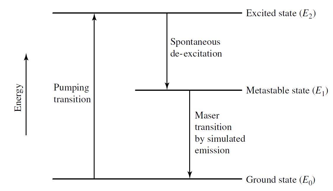
Fig. 9.11 A schematic diagram of a hypothetical three-level maser. (Carroll & Ostlie (2007))#
9.2.11. Post-Asymptotic Giant Branch#
AS the clout around the OH/IR source expands, it eventually becomes optically thin and exposes the central star, which exhibits a spectrum of an F or G supergiant. The \(1-5\,M_\odot\) stars evolve blueward, where they leave the TP-AGB and move nearly horizontally across the H-R diagram as post-AGB stars. During the final phase of mass loss, the remainder of the star’s envelope is expelled. With only a very thin layer of material remaining, the hydrogen- and helium-burning shells are extinguished causing the luminosity of the star to drop rapidly. The hot central object will cool to become a white dwarf star, which is essentially the red giant’s degenerate \({\rm CO}\) core (or \({\rm ONeMg}\) cores for more massive stars) and surrounded by a thin layer of residual hydrogen and helium.

Fig. 9.12 The AGB and post-AGB evolution of a 0.6 \(M_\odot\) star undergoing mass loss. The initial composition of the model is \(X = 0.749\), \(Y = 0.25\), and \(Z = 0.001\). (Carroll & Ostlie (2007); Data from Iben, Ap. J., 147, 624, 1967.)#
9.2.12. Planetary Nebulae#
The expanding shell of gas around a white dwarf progenitor is called a planetary nebula. These glowing gas clouds were given this name in the 19th century because they looked somewhat like giant gaseous planets when viewing through a small telescope. A planetary nebular owes its appearance to the UV light emitted by the hot, condensed central star. The UV photons are absorbed bye the surrounding gas in the nebula, which causes the atoms to become excited or ionized. When the electrons cascade back down to lower energy levels, photons are emitted whose wavelengths are in the visible.
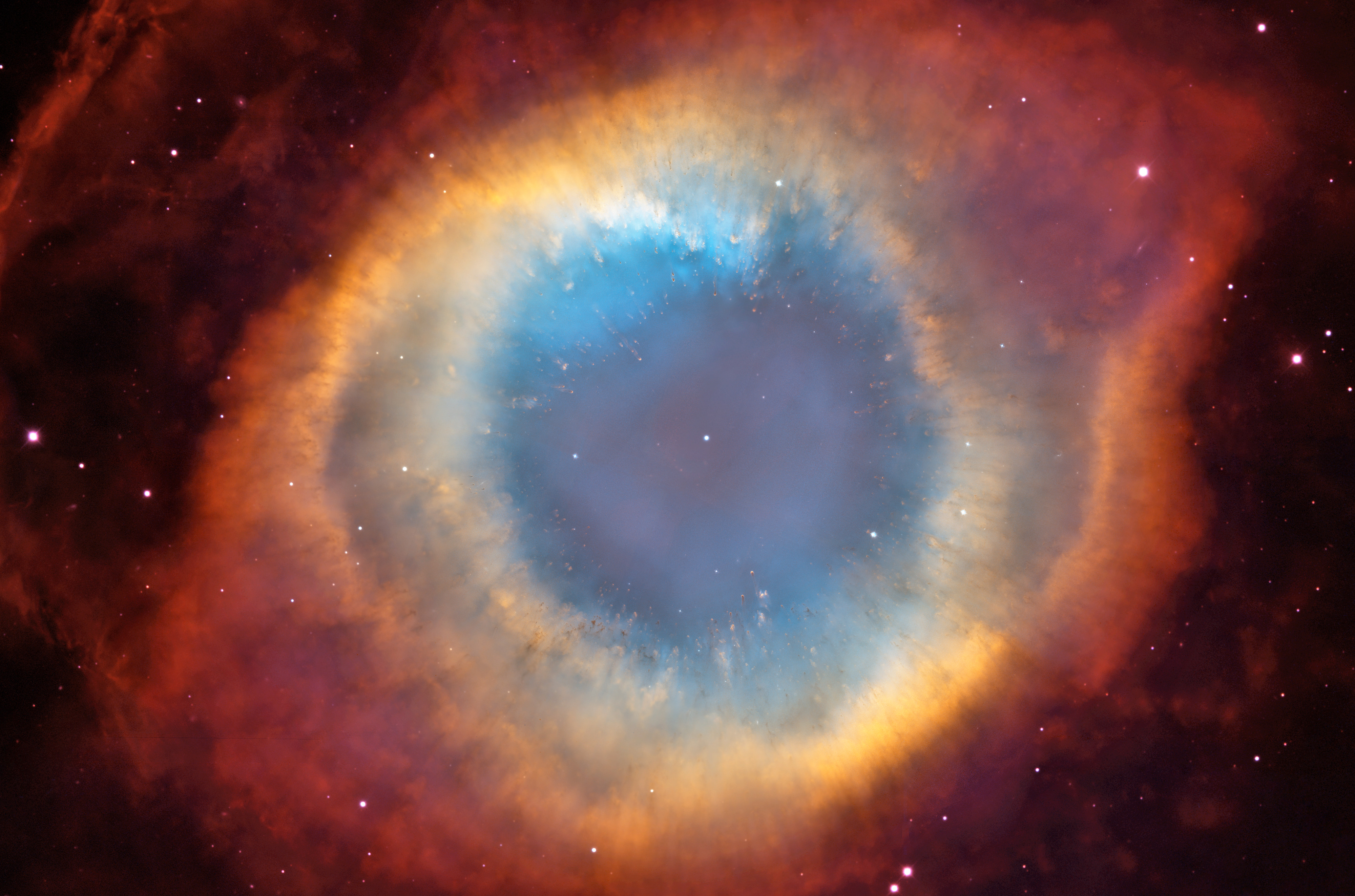
Fig. 9.13 The Helix nebula (NGC 7293) is one of the closest planetary nebulae to Earth, 213 pc away in the constellation of Aquarius. (Credit: NASA, ESA, C.R. O’Dell (Vanderbilt University), and M. Meixner, P. McCullough, and G. Bacon (STScI))#

Fig. 9.14 A close-up of “cometary knots” in the Helix nebula. (Credit: NASA, C. Robert O’Dell and Kerry P. Handron (Rice University))#
With high-resolution images, astronomers have realized that the morphologies of the planetary nebulae are often much more complex than the spherically symmetric parent TP-AGB star. The Helix nebula looks as though it has a ringlike structure because the gas is ejected preferentially along the equator of the star due to the presence of angular momentum and our viewing angle is down the star’s rotation axis. Nebula differ in structure due to the varying viewing angles, multiple ejections of material from the stellar surface, the presence of companion stars, and magnetic fields.

Fig. 9.15 NGC 6543 (the “Cat’s Eye”) is a planetary nebula in Draco, 900 pc away. (Credit: ESA, NASA, HEIC and The Hubble Heritage Team (STScI/AURA))#
The expansion velocities of planetary nebulae (as measured by Doppler-shifted spectral lines) show that the gas is typically moving away from the central star with speeds between \(10-30\,{\rm km/s}\), although much greater speeds have been measured. Combined with characteristic length scales of around 0.3 pc, their estimated ages are \({\sim}\text{10,000}\) yr. After 50,000 yr, a planetary nebula will dissipate into the ISM. Despite their short lifetime about 1500 planetary nebulae are known to exist in the Milky Way Galaxy. Given the observational biases, the estimate should be an order of magnitude bigger (15,000 planetary nebulae).
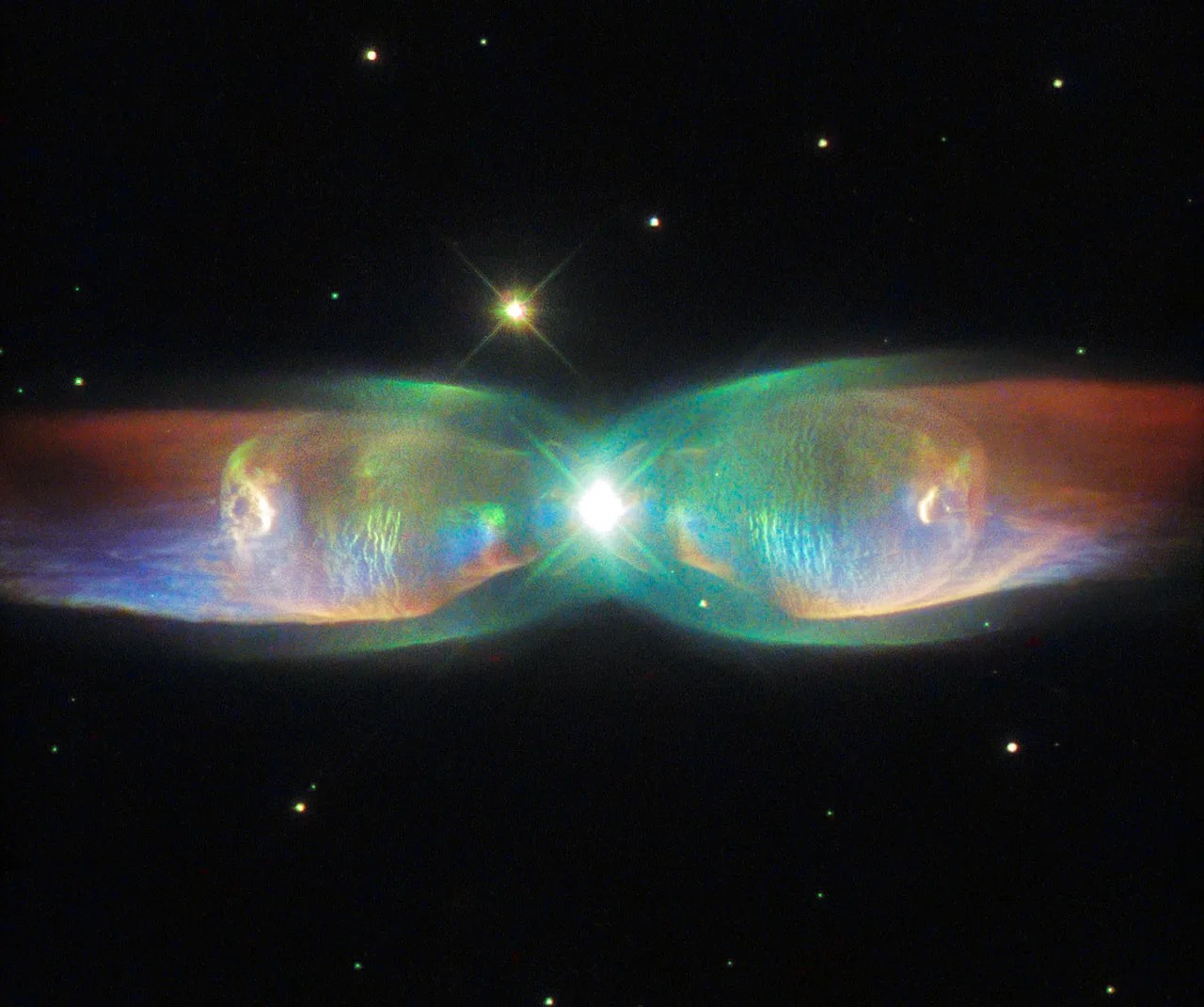
Fig. 9.16 The Twin Jet Nebula, or PN M2-9, is a striking example of a bipolar planetary nebula. (Credit: ESA, NASA, HEIC and The Hubble Heritage Team (STScI/AURA); processing Judy Schmidt)#
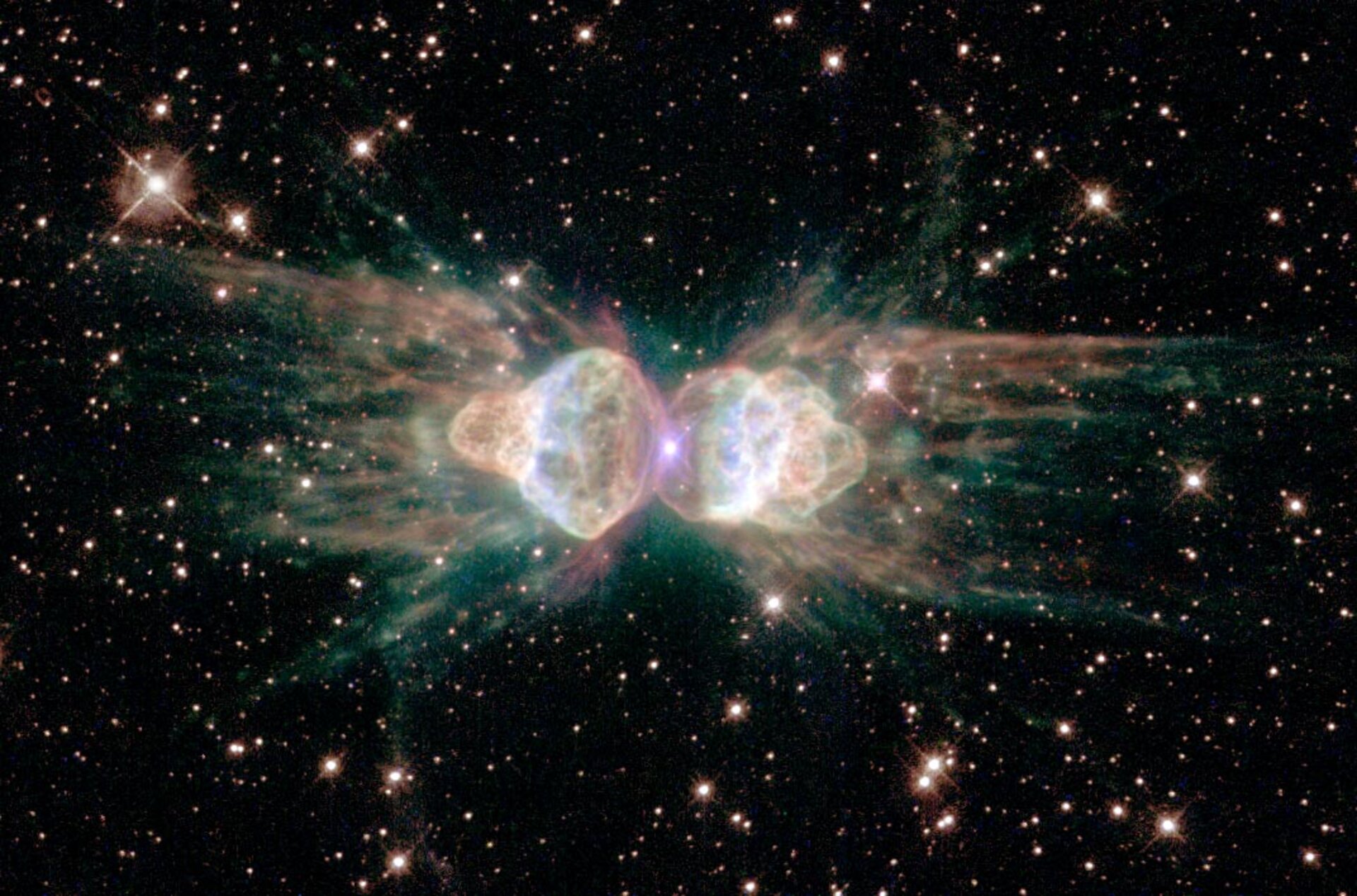
Fig. 9.17 From Earth, Menzel 3 resembles the head and thorax of a common garden ant, hence its name. (Credit: ESA, NASA, HEIC and The Hubble Heritage Team (STScI/AURA))#
9.3. Stellar Clusters#
9.3.1. Population I, II, and III Stars#
The universe began with the Big Bang about 13.7 Gyr ago. In the beginning, almost all the elements in the universe were either the hydrogen or helium produce through nucleosynthesis of the Big Bang itself. The first stars to form had no metal content \((Z=0)\), where the next generation of stars were extremely metal-poor have very small, but non-zero values of \(Z\). Successive generations of stars resulted in higher proportions of heavy elements available during their own formation, which leads to more metal-rich stars \((Z=0.03)\). Stars are classified as populations using their metal content, which is also a proxy for how long after the Big Bang they likely formed. These populations are:
Population III stars are the original stars that formed immediately after the Big Bang; \(Z=0\).
Population II stars are metal-poor; \(Z\gtrsim 0\). Population II stars can be found well above or below the disk of the Milky Way.
Population I stars are metal-rich; \(Z>0\). These stars have relative velocities (to the Sun) that are low compared to Population II stars. Furthermore, they are found predominantly in the disk of the Milky Way.
The classifications of Population II and I are originally due to their kinematically distinct groups of stars within our Galaxy. It was only later that astronomers realized that these two groups differed chemically as well.
9.3.2. Globular Clusters and Galactic (Open) Clusters#
During the collapse of a molecular cloud, stellar cluster can form that range in size from \(10-10^5\) stars. Every member of a given cluster formed
from the same cloud,
with essentially identical compositions, and
within a relatively short period of time.
Excluding effects like rotation, magnetic fields, and binary star membership, the Vogt-Russell theorem suggests that solely their initial masses explain the differences in each cluster member’s evolutionary state.
Extreme Population II cluster formed when the Milky Way Galaxy was very young, which makes them some of the oldest objects in the Galaxy. They also contain the largest number of members. Globular clusters are Population II objects and M13 (located in the constellation Hercules) is an example. Population I clusters (e.g., the Pleiades) tend to be smaller, younger, and bluer. These smaller clusters are called open clusters.

Fig. 9.18 M13, the great globular cluster in Hercules, is located approximately 7000 pc from Earth. (Credit: Adam Block, Mt. Lemmon SkyCenter, U. Arizona)#
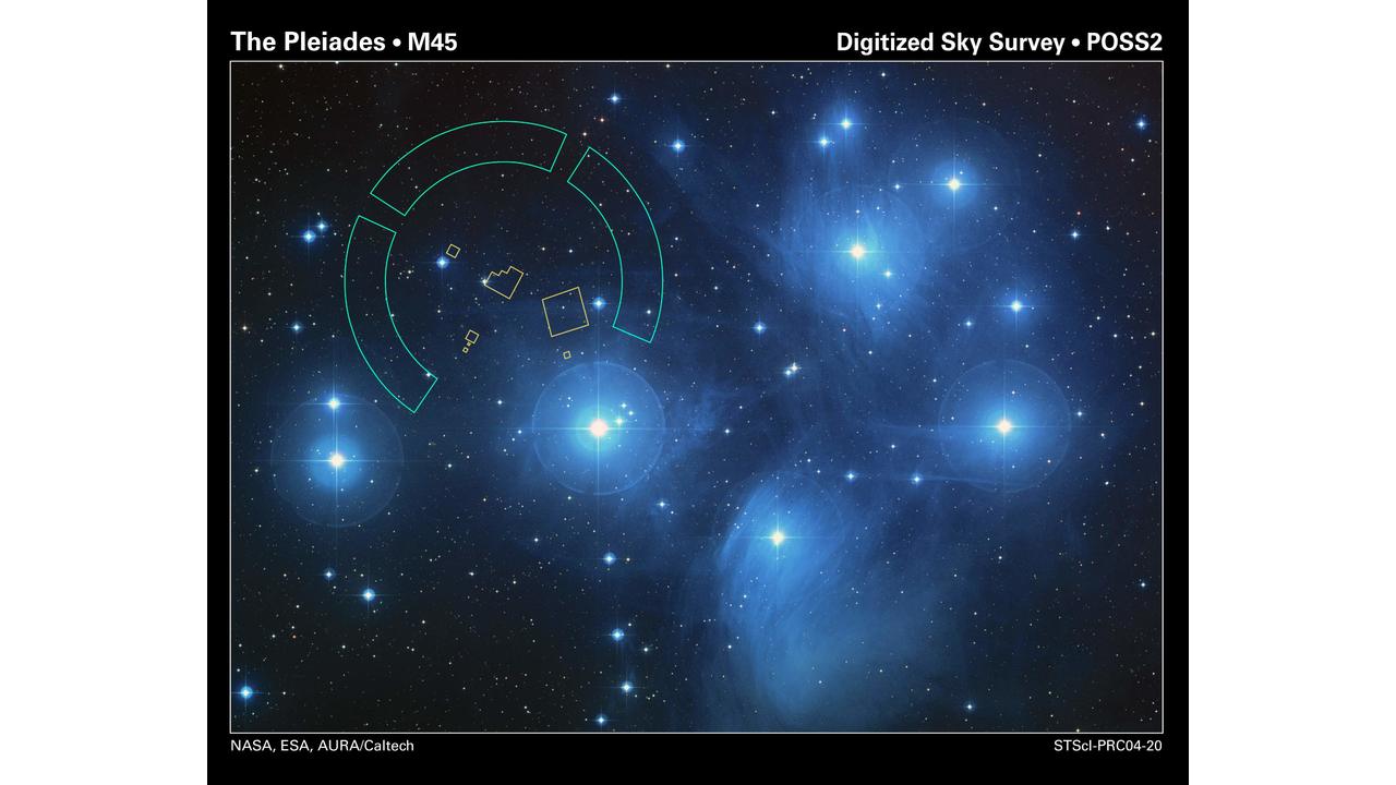
Fig. 9.19 The Pleiades is a galactic cluster found in the constellation of Taurus, at a distance of 130 pc. (Credit: ESA, NASA, Aura and CalTech)#
9.3.3. Spectroscopic Parallax#
The H-R diagrams of cluster can be constructed in a self-consistent way without knowledge of the exact distances to them. The interstellar distances within a cluster are small relative to the cluster’s distance from Earth and thus, little error is introduced by assuming that each member has essentially the same distance modulus. Plotting the apparent magnitude instead of the absolute magnitude only amounts to a vertical shift of each star in the diagram. By matching the main-sequence stars to a main-sequence calibrated in absolute magnitude allows one to determine the distance modulus (i.e., the vertical shift between the two curves). this method of distance determination is known as spectroscopic parallax, or main-sequence fitting.
9.3.4. Color-Magnitude Diagrams#
Rather than attempting to determine the effective temperature of every member of a cluster, it is much faster to determine their color indices \(B-V\). With the knowledge of apparent magnitude and the color index of each star, a color-magnitude diagram can be constructed with the apparent magnitude \(V\) along the y-axis and the color index \(B-V\) along the x-axis.

Fig. 9.20 A color–magnitude diagram for M3, an old globular cluster. (Carroll & Ostlie (2007); Figure adapted from Renzini & Fusi Pecci. Annu. Rev. Astron. Astrophys. 26, 199, 1988.)#
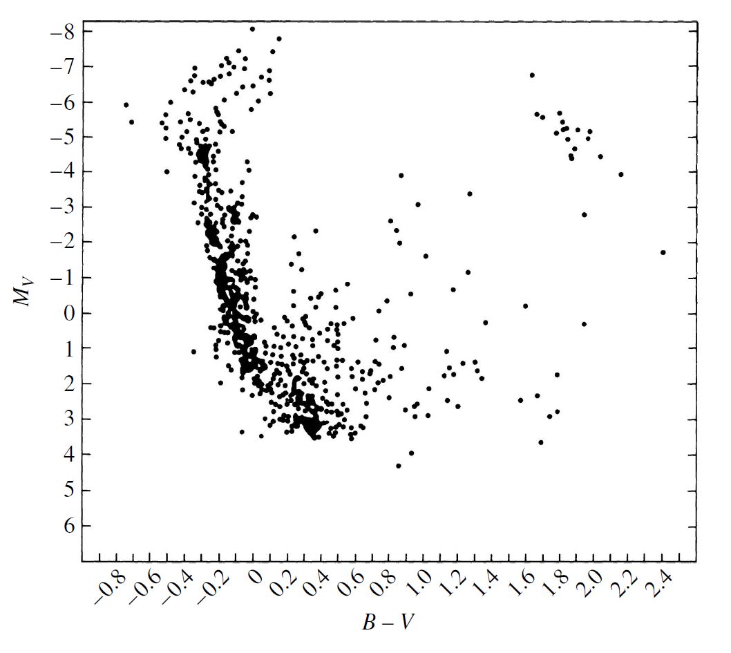
Fig. 9.21 A color–magnitude diagram for the young double galactic cluster, \(h\) (NGC 869) and \(\chi\) (NGC 884) Persei. (Carroll & Ostlie (2007); Figure adapted from Wildey, ApJS, 8. 439, 1964.)#
9.3.5. Isochrones and Cluster Ages#
Clusters offer near ideal tests of many aspects of stellar evolution theory due to their color-magnitude diagrams that are correlated with a H-R diagram. By computing the evolutionary tracks of many stars (with a range of mass) that all have the same composition, it is possible to plot the position of each evolving model on the H-R diagram when the model reaches the age of the cluster. The curve connecting these positions is known as an isochrone. The relative number of stars at each location depends on the number of star in each mass range with the cluster (i.e., the initial mass function), combined with the different evolutionary rates during each phase.
As the cluster ages, the most massive and least abundant stars will arrive on the main sequence first and evolve rapidly. Before the lowest-mass stars reach the main sequence, the most massive ones have already evolved off the main sequence into the red giant region (perhaps even undergoing supernova explosions). Core hydrogen-burning lifetimes are inversely related to mass, which means the remaining main-sequence stars mark a turn-off point. The cluster becomes redder and less luminous with time. It is also possible to estimate the age of a cluster by the location of the turn-off point or the uppermost point of its main sequence.
9.3.6. The Hertzsprung Gap#
Another consequence of varying timescales can be seen in the color-magnitude diagrams of \(h+\chi\) Persei. Apparent are red giants, low-mass main sequence stars, and a population of very red \((B-V\sim 1.75)\) giants. It is unlikely that this represents an incomplete survey, since the stars are the brightest members of the cluster. It points out the very rapid evolution that occurs just after leaving the main sequence and is known as the Hertzsprung gap. The existence of the Hertzsprung gap is due to the evolution on a Kelvin-Helmholtz timescale across the SGB following the core contraction at the Schöberg-Chandrasekhar limit. The clusters M67 and M3 do not show the existence of the Hertzsprung gap because the rapid contraction phase (below \(1.25\,M_\odot\)) related to the Schöberg-Chandrasekhar limit is less pronounced. Color-magnitude diagrams of old globular clusters with turn-off points near or less than a Solar-mass have continuous star distributions leading to the red giant region.

Fig. 9.22 A composite color–magnitude diagram for a set of Population I galactic clusters. (Carroll & Ostlie (2007))#
9.3.7. Blue Stragglers#
A group of stars, known as blue stragglers, can be found above the turn-off point of M3. It appears that their tardiness (in leaving the main sequence) is due to an unusual aspect of their evolution, where the most likely scenarios appear to be:
mass exchange with a binary star companion, or
collisions between two stars,
which extends the star’s main-sequence lifetime.
9.4. Homework#
Problem 1
Construct a table that expresses the evolutionary times between points 2 and 3, points 3 and 4, and so on, as a percentage of the lifetime of the star on the main sequence between points 1 and 2. Use the Table associated with Fig. 9.1 for a 5 \(M_\odot\) star.
(a) How long does it take a 5 \(M_\odot\) star to cross the points 3 and 5 relative to its main-sequence lifetime?
(b) How long does a 5 \(M_\odot\) star spend on between points 7 and 8 relative to its main-sequence lifetime?
(c) How long does a 5 \(M_\odot\) star spend on between points 8 and 9 relative to its main-sequence lifetime?
Problem 2
Show that the radius of the isothermal core for which the gas pressure is a maximum is given by Eq. (9.8). Recall that this solution assumes that the gas in the core is ideal and monatomic.
Problem 3
The age of the universe is 13.7 Gyr. Compare this value to the main-sequence lifetime of a 0.8 \(M_\odot\) star. Why isn’t it useful to compute the detailed post-main-sequence evolution of stars with masses much lower than the mass of the Sun?
Problem 4
Estimate the Kelvin–Helmholtz timescale for a 5 \(M_\odot\) star on the subgiant branch and compare your result with the amount of time the star spends between points 4 and 5 in Figure 9.1.
Problem 5
The Helix nebula is a planetary nebula with an angular diameter of 16’ that is located approximately 213 pc from Earth.
(a) Calculate the diameter of the nebula.
(b) Assuming that the nebula is expanding away from the central star at a constant velocity of \(20\,{\rm km/s}\), estimate its age.