3. Telescopes#
3.1. Basic Optics#
The development of optics greatly enhanced our window into the universe starting with Galileo’s innovative use of the telescope. Today we “see” with many different sets of eyes to get a fuller picture of the cosmos, discover faint objects otherwise unseen, and resolve distant objects in greater detail.
3.1.1. Refraction and Reflection#
The first “telescope” was developed by Hans Lippershey in 1608 and a year later Galileo Galilei built his own version with about \(3\times\) magnification and later improved upon the design to obtain a version with \(30\times\) magnification. These refracting telescopes consisted of lenses through which the light would pass and form an image. In 1671, Isaac Newton showed that any refracting telescope would suffer from the dispersion of light into colors and he developed the reflecting telescope that used a mirror instead of a lens to bypass the problem.
Both types of telescopes use a lens to produce an image, which makes a natural starting point. Snell’s law of refraction describes how the path of a light ray changes as it travels through a lens. When a wave travels across a boundary between two media, its path is bent (refracts) at the interface.
The amount that the ray bends is material dependent and characterized by a wavelength-dependent index of refraction \(n_\lambda = c/v_\lambda\), where \(v_\lambda\) represents the speed of light within the medium.
Alternatively, the index of refraction indicates how much the speed of light decreases within the medium (\(v_\lambda = c/n_\lambda\)) compared to vacuum.
Note that the frequency \(\nu\) of the wave remains unchanged and the refracted wavelength must change.
The incoming ray possesses an angle of incidence \(\theta_i\) and the refracted ray is bent by \(\theta_r\), where both angles are measured relative to the normal to the interface. Then Snell’s law is given by

Fig. 3.1 Refraction of light at the interface between two media. Image credit: Wikipdeia:Snell’s Law.#
Exercise 3.1
Green light (\(\lambda_{\rm air} = 540\) nm) is incident from air to glass (\(n=1.51\)). - (a) What is the wavelength of light in the glass? - (b) If \(\theta_i = 37^\circ\), what is the angle of refraction?
To determine the wavelength of light in the glass, we apply the law of refraction:
where \(n_{\rm air}\), \(n_{\rm g}, \)\lambda_{\rm air}\(, and \)\lambda_{\rm f}$ represents the index of refraction in air, index of refraction in the glass, wavelength in the air, and wavelength in the glass, respectively.
Given the angle of incidence \(\theta_i\), the angle of refraction can be determined via Snell’s law. Mathematically, this is
where \(\theta_i\) must be converted from degrees to radians and the final result converted from radians back to degrees.
import numpy as np

def refract_lambda(l,n1,n2):
    #l = lambda; wavelength in medium 1
    #n1 = index of refraction of medium 1
    #n2 = index of refraction of medium 2
    return l*(n1/n2)

def snell_law(th1,n1,n2):
    #th1 = angle in medium 1 (relative to normal) in radians
    #n1 = index of refraction of medium 1
    #n2 = index of refraction of medium 2
    return np.arcsin((n1/n2)*np.sin(th1))

lambda_air = 540
n_air = 1.00029
n_glass = 1.51
theta_i = np.radians(37)
print("The wavelength in glass is %3d nm." % (refract_lambda(lambda_air,n_air,n_glass)))
print("The angle of refraction is %2.1f deg." % np.degrees(snell_law(theta_i,n_air,n_glass)))
The wavelength in glass is 357 nm.
The angle of refraction is 23.5 deg.
Lenses are shaped from glass so that the light rays can converge or diverge due to Snell’s law. The light rays are traced where the lens is set perpendicular to the horizontal (or optical axis) to produce an axis of symmetry.
Converging lenses force the light rays to come to a point on the optical axis (opposite from the incoming rays). This unique point is called the focal point of the lens and the distance to that point from the center of the lens is called the focal length \(f\).
By changing the curvature of the lens, the light rays can instead diverge from the optical axis to make a diverging lens. As a result, the focal point lies on the same side as the incoming rays. For a converging lens , the focal length is defined as positive, where the focal length is negative for a diverging lens.
The focal length \(f_\lambda\) of a thin lens can be calculated from the index of refraction \(n_\lambda\) and the radii of curvature of each surface (\(R_1\) and \(R_2\)) assuming the surfaces are spheroidal. The sign convention for the radii is positive (convex) and negative (concave). The focal length is given by the lensmaker’s formula,
For mirrors, the focal length \(f\) is wavelength-independent since the light rays do not penetrate the surface and angle of reflection is equal to the angle of incidence (\(\theta_i = \theta_r\)). A spheroidal mirror has a focal length at half the radius of curvature (\(f=R/2\)) and can be positive/negative depending on the geometry. Converging mirrors are generally used as the primary mirror in modern telescopes, although diverging or flat mirrors may be used for more complicated optical systems.
3.1.2. The Focal Plane#
To record an image, the detector must be placed in the focal plane of the telescope, which is defined as the plane passing through the focal point and oriented perpendicular to the optical axis of the system. The image separation of two point sources on the focal plane is relate to the focal length. At the position of the focal plane, the rays from the on-axis source will converge at the focal point while the rays fro the other source will approximately meet a distance \(y\) from the focal point.
Using the geometry of a triangle with a long side \(f\) and angle \(\theta\) (incoming light rays from the source relative to the optical axis), the short side \(y\) can be determined by
The field of view for the telescope is typically small so that the angle \(\theta\) is also small. For a sufficiently small \(\theta\), the small-angle approximation (\(\tan\theta \approx \theta\)) can be used to give
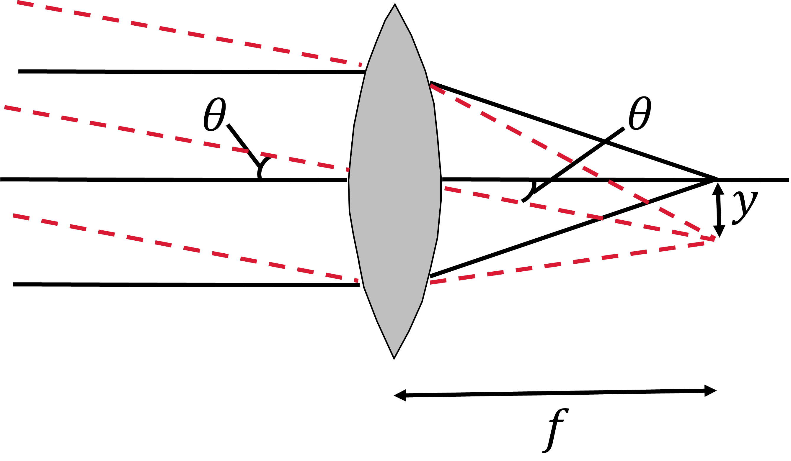
Fig. 3.2 The plate scale \(y\) determined by the focal length \(f\) of the system.#
This leads to the plate scale (\(d\theta/dy = p = 1/f\)), which connects the angular separation of the objects on the sky with the linear separation of their images at the focal plane. The plate scale is typically given in arcseconds/mm due to the history of using of photographic plates. The plate scale of JWST’s fine guidance sensor is about 0.065\(^{\prime\prime}\) per pixel.
3.1.3. Resolution and the Rayleigh Criterion#
To resolve two closely spaced objects, its not simply a matter of choosing a sufficiently long focal length. There is a fundamental limit to our ability to resolve the objects due to the diffraction produced by the advancing wavefronts from each object. This phenomenon is related to the single slit diffraction pattern produced by a slit of width \(D\).
Any ray passing through the opening (or aperture) and arriving at a specific point can be though of as being associated with another ray passing through the aperture a distance of \(D/2\) away and arriving at the same point. If the two rays are a half-wavelength (\(\lambda/2\)) out of phase, then destructive interference will occur. This leads to the relation
where \(m = 1,2,3,\ldots\) for dark fringes. If a circular aperture is used (i.e., a telescope) the symmetry produces a series of concentric rings instead of the iconic diffraction pattern. The mathematics of this pattern was solved by George Airy in 1835 and is known as the Airy disk. If we relax Eq. (3.4) so that \(m\) is no longer an integer, then it can be used to find the maxima as well.
Two sources that are sufficiently close together will have diffraction rings that overlap and it becomes impossible to resolve. The two images are said to unresolved when the central maximum of one pattern falls inside the location of the first minimum of the other, where this condition is the Rayleigh criterion. Assuming that angular separation \(\theta_{\rm min}\) is quite small and invoking the small-angle approximation, the Rayleigh criterion is given by
for a circular aperture, where \(\lambda\) is the wavelength of light and \(D\) is the diameter of the telescope’s primary mirror. Ground-based telescopes rarely approach the theoretical limit without assistance through adaptive optics due to the turbulence of the atmosphere or “seeing”. Local conditions affect the degree of twinkling observed, where observatories high above sea level (“above the weather”) provide the best observing conditions.
Exercise 3.2
A single slit of width D = 0.1 mm is illuminated by light through a visual Johnson filter and diffraction bands are observed on a screen 0.5 m from the slit. How far is the third dark band from the central bright band?
The peak wavelength of the visual Johnson filter is \(550\ {\rm nm}\), which we can use to determine the distance of the third (\(m=3\)) dark band relative to the central bright band for a single slit diffraction. From Eq. (3.4), we solve for the diffraction angle \(\theta\) as
where the final result is converted from radians to degrees. The distance to the third band is \(0.5\tan{\theta} = 0.008\ {\rm m}\), or \(8\ {\rm mm}\).
Exercise 3.3
What is the diffraction limit (in arcseconds) for JWST’s fine guidance sensor (FGS) at 5 \(\rm \mu m\)?
The diffraction is determined using the Rayleigh criterion (Eq. (3.5)), where we use the NASA specifications for the effective diameter of JWST (\(D= 6.5\ {\rm m}\)) and the peak wavelength sensitivity \((\lambda = 5\ {\rm \mu m})\) for the FGS. Substituting these values, we get
where the final result is converted from radians to arcseconds.
def single_slit_th(D,l,m):
    #D = slit width
    #l = lambda; wavelength of light; must match units with D
    #m = order of dark fringes
    return np.arcsin(m*l/D) #return theta in radians

def diff_limit(D,l):
    #D = aperture size
    #l = lambda; wavelength of light
    return (1.22*l/D)*(180/np.pi)*3600 #return theta_min in arcseconds
D_slit = 0.1*1e-3 #converted to m
V_johnson = 550*1e-9 #converted peak visual wavelength to m
th_diff = single_slit_th(D_slit,V_johnson,3)
print("The diffraction angle of the third dark band is %2.1f deg." % np.degrees(th_diff))
print("The distance from the central bright band is %1.3f m." % (0.5*np.tan(th_diff)))

D_JWST = 6.5 #diameter of primary mirror
l_FGS = 5*1e-6 #converted to m

print("The diffraction limit for JWST's FGS at 5 um is %2.2f arcsec." % diff_limit(D_JWST,l_FGS))
The diffraction angle of the third dark band is 0.9 deg.
The distance from the central bright band is 0.008 m.
The diffraction limit for JWST's FGS at 5 um is 0.19 arcsec.
3.1.4. Aberrations#
Image distortions or aberrations affect both lens and mirror systems. Refracting telescopes suffer from chromatic aberration, which is a distortion due to the wavelength-dependent focus of a lens. The lensmaker’s formula (Eq. (3.2)) depends on the radii of curvature and the index of refraction \(n\), but \(n\) also depends on the wavelength \(\lambda\). This translates into a wavelength-dependent focal length, where the focal point for red light is different than for blue light.
There can be aberrations that result from the shape of the reflecting or refracting surface. Imperfections in the grinding/polishing of lens/mirrors mean not all areas will focus a parallel set of light rays to a single point. This type of distortion is called spherical aberration and can be overcome with a corrective lens. The Hubble Space Telescope (HST) initially had imaging problems due to spherical aberration when a mistake was made while grinding the primary and left the center of the mirror too shallow by about 2 \(\mu m\). A repair mission in 1993, installed a special corrective optics package on the telescope.
A coma produces elongated images of a point sources that lie off the optical axis. An astigmatism is a defect where different parts of a lens or mirror converge an image a slightly different locations on the focal plane. Correcting for astigmatism can create other problems, such as the curvature of field that is due to the focusing of images on a curve rather than on a flat surface.
3.1.5. Brightness of an Image#
It might be assumed that the brightness of an extended (resolved) image depends on the area of the aperture. This is the case for photography, where the camera has an adjustable aperture (iris) that controls how much light enters the camera to reach the detector on the focal plane. For most astronomical applications, the aperture is fully open because the object is effectively infinitely far away (i.e., distance \(r \gg \) focal length \(f\)). Then, it can be shown that the intensity of the radiation is the same for both the object and image; independent of the area of the aperture. The exception is for bright objects (e.g., the Moon), where an adjustable iris helps prevent over-exposing the image (i.e., saturation).
The light-gathering power of telescopes is the illumination \(J\) or the number of photons per second that are focused onto a unit area of a resolved image. When comparing telescopes, the amount of light collected is proportional to the area of the aperture or the illumination \(J \propto \pi D^2/4\), where \(D\) is the diameter of the telescope’s aperture. Through the plate scale (Eq. (3.3)) we have the linear size of the image proportional to the focal length of the lens and the image area is proportional to \(f^2\). The illumination is proportional to the ratio of the aperture diameter \(D\) to the focal length \(f\) (i.e., \(J\propto D^2/f^2\)). The inverse of the ratio is ofter referred to as the focal ratio (or f-ratio),
The illumination indicates the amount of time required to collect the photons needed to form a bright image. A larger focal ratio corresponds to a slower telescope, which means that a longer exposure is necessary to reach an equivalent illumination.
Exercise 3.4
The twin telescopes of the Keck Observatory at Mauna Kea have primary mirrors 10 m in diameter with focal lengths of 17.5 m. What is the focal ratios of each telescope?
The f-ratio of a telescope is the ratio of the focal length \(f\) with the telescope’s diameter \(D\). Each of the twin Keck telescopes have a focal length of 17.5 m with a 10 m primary mirror. We calculate the f-ratio as
def F_ratio(f,D):
    #f = focal length of the telescope
    #D = diameter of the telescope aperture; must match units with f
    return f/D

print("The focal ratio of each telescope is f/%1.2f." % F_ratio(17.5,10))
The focal ratio of each telescope is f/1.75.
3.2. Optical Telescopes#
3.2.1. Refracting Telescopes#
The major optical component of a refracting telescope is the primary (or objective) lens with a focal length \(f_{\rm obj}\). The objective lens collects the light and brings the light to a focus at the focal plane, where a photographic plate or other detector can be placed at the focal plane to record the image. The eyepiece serves as a magnifying glass and would be placed a distance from the focal plane equal to its focal length \(f_{\rm eye}\). The path of rays coming from a point source lying off the optical axis (at an angle \(\theta\)) ultimately emerge from the eyepiece an an angle \(\phi\) from the optical axis.
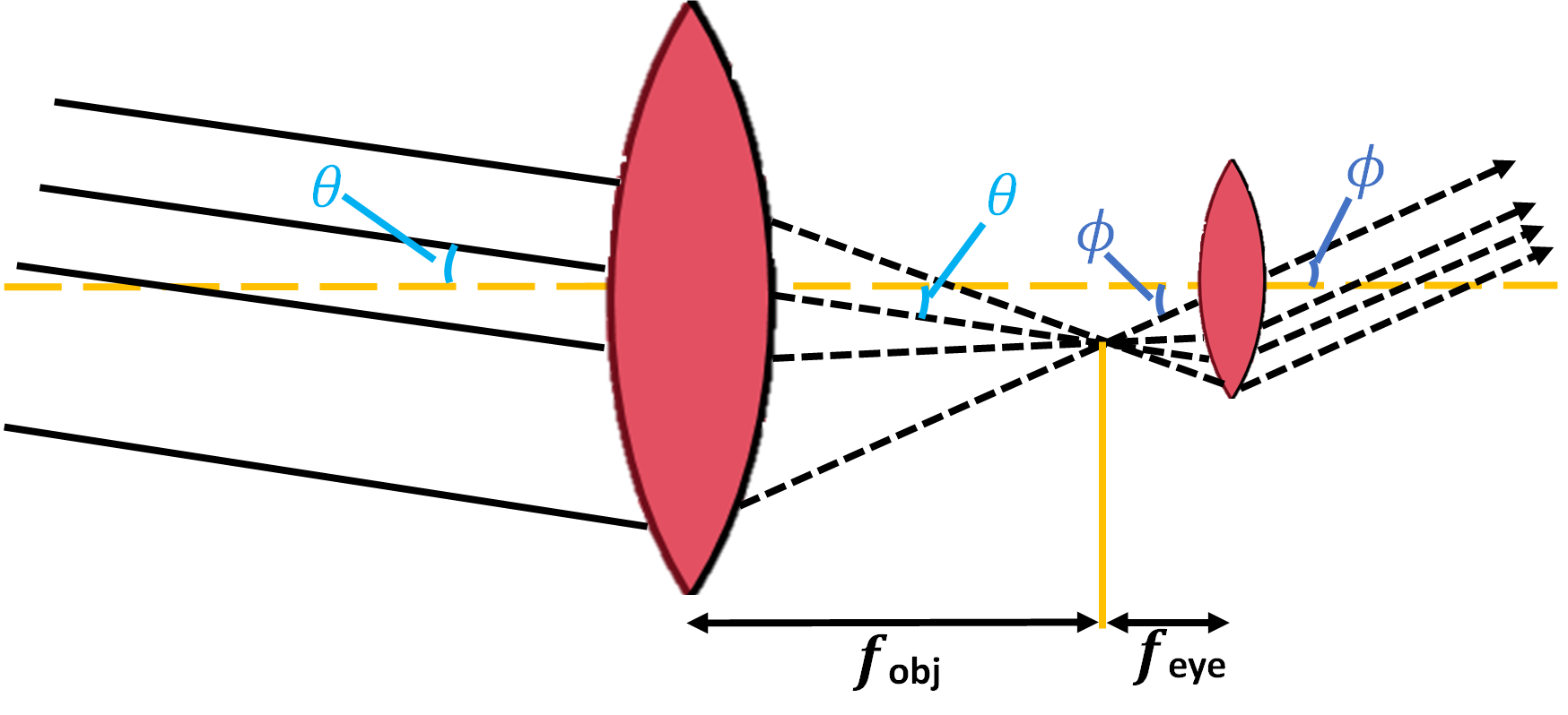
Fig. 3.3 A refracting telescope is composed of an objective lens and an eyepiece.#
The angular magnification produced by this arrangement of lenses can be shown to be
where a review is available in OpenStax:College Physics. Since the objective lens tends to be a fixed part of the telescope, several eyepieces (of different focal lengths) can be used to produce different angular magnifications. Note that viewing a large image requires a long objective in combination with a short focal length for the eyepiece.
Recall that the illumination is inversely proportional to the square of the objective’s focal length and a larger diameter objective is needed to compensate. However, there are practical limitations for to the size of a refracting telescope’s objective. The lens is supported only around its edges and the shape of the lens deforms due to gravity when the size and weight are increased. Furthermore, the type of deformation changes as the orientation of the telescope varies.
Another limitation is the construction of the lens, which can have defects. The light must pass through the entire volume of the lens and the quality must be nearly optically perfect. Defects in the desired shape of the lens must be kept to a small fraction (\(\lambda/20\)) of the wavelength (\(\lambda = 400-700\) nm for visible light). A large objective lens also has a slow thermal response, where the telescope must adjust to the temperature of the outside air after the dome is opened. Thermally driven air currents develop around the telescope, which compound the normal concerns around “seeing”. The overall shape of the telescope will change as a consequence of thermal expansion, which alters the optical alignment.
Considering all of these challenges (along with the unique problem of chromatic aberration), the vast majority of all large modern telescopes are reflectors. The largest refracting telescope in use today is at the Yerkes Observatory in Williams Bay, Wisconsin. It has a 40-in (1.02 m) objective with a focal length of 19.36 m.
3.2.2. Reflecting Telescopes#
A reflecting telescope is designed by replacing the objective lens with a mirror, which either reduces or eliminates many of the problems with refracting telescopes. The light does not pass through a mirror and thus, much less precision is required in its construction (i.e., only one surface needs to be ground with precision). The weight of the mirror can be minimized by using a lighter honeycomb structure behind the reflecting surface. As a result, parts of the mirror can be mechanically deformed to correct for thermal and/or gravitational effects as the telescope moves (i.e., adaptive optics).
Although there are many benefits in using a mirror, there are some costs. The primary mirror reflects the light back along the optical axis (i.e., law of reflection) to the focal point (i.e., prime focus). A detector can be placed at this location, but some of the incident light is blocked. Additionally, the structure supporting the detector introduces diffraction spikes in the image of the stars. Isaac Newton found a solution to the problem of the prime focus by placing a small, flat mirror in the reflected light’s path changing the location of the focal point. A Newtonian telescope design suffers a mechanical cost because the eyepiece (or detector) must be placed a significant distance from the telescope’s center of mass and would exert a significant torque on the telescope.
The secondary mirror effectively produces a shadow on the primary mirror (rendering a small area useless) and a hole can be bored into the primary mirror so that the reflected light comes through the hole. This Cassegrain design makes it possible to place a massive detector near the telescope’s center of mass and the observer can stay near the bottom of the telescope. The secondary mirror is usually convex, while the primary mirror is concave . However, a Ritchey-Chrétien has a hyperbolic primary mirror rather than a parabolic one. The Ritchey-Chrétien design has a wider field of view and eliminates off-axis optical errors (coma). Some well-known examples are the Hubble Space Telescope, the Keck telescopes and the ESO Very Large Telescope.
If the instrument package is too massive, astronomers use a series of mirrors to reflect the light down the telescope’s mount to a coudé room located below the telescope (i.e., coudé telescope). Because of the extended optical path, a very long focal length is needed and is particularly useful in spectral line studies. A modification of the Cassegrain design uses a spheroidal primary mirror (to minimize coma) combined with a “correcting” lens to help remove spherical aberration. The benefit of a Schmidt-Cassegrain telescope is a wider field of view and is important for survey studies of large regions of sky.
3.2.3. Adaptive Optics#
While large-aperture ground-based telescopes have a larger light-gathering power than small telescopes, they are still limited in resolving power due to thermal fluctuations of the atmosphere. Even the Keck telescopes at Mauna Kea cannot resolve a source any better than a 0.2 m telescope without the aide of active optics to correct the distortions in the telescope’s mirrors and adaptive optics to compensate for atmospheric turbulence. A small deformable (“rubber”) mirror is used with many piezoelectric crystals attached to the back. To counteract changes in the shape of wavefronts due to Earth’s atmosphere, the crystals make \(\mu m\)-size adjustments to the shape of the mirror several hundred times per second. To make the needed adjustments, the telescope monitors a guide star that is very near the target.
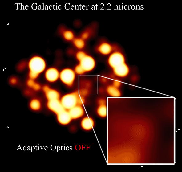
Fig. 3.4 The Galactic Center at 2.2 \(\rm \mu m\). Image credit: UCLA Galactic Group#
3.2.4. Space-based Observatories#
To overcome the imaging problems imposed by Earth’s atmosphere, observational astronomy has made leaps through observatories on satellites in space. The Hubble Space Telescope has a 2.4 m (f/24) primary using a Ritchey-Chrétien design, where long exposures of 150+ hours allow the telescope to detect objects as faint as \(m_V = +30\). On December 25, 2021 the James Webb Space Telescope (JWST) was launched on an Ariane 5 rocket. This telescope has a 6.5 m primary and will orbit at the Earth-Sun Lagrange point (L2). This location was chosen for the spacecraft to minimize thermal emissions that would affect its IR detectors.
3.2.5. Electronic Detectors#
For most of history, the human eye was the main tool of an astronomer to identify the stars for rituals, navigation, and agriculture. Photographic plates were developed at the end of the 19th century and became a mainstay for astronomers through much of the 20th century due to there persistence of vision. Today, the semiconductor device known as the charge-coupled device (CCD) revolutionized the counting of photons (through process similar to the photoelectric effect). CCDs are able to detect nearly 100% of the incident photons over a very wide range of wavelengths. CCDs also have a wide dynamic range, where they can differentiate between very bright and dim objects viewed simultaneously.
A CCD works by collecting electrons that are excited into higher energy states (conduction bands) when a detector is struck by a photon. The number of electrons collected in each pixel is proportional to the image brightness. HST’s Wide Field and Planetary Camera (WF/PC 2) has 2.5 million pixels with each pixel capable of holding up to 70,000 electrons. A very bright target (e.g., \(\alpha\) Cen AB (Brice-Olivier et al. 2015)) requires a fast shutter so that the pixels don’t saturate (i.e., overflow with electrons).
3.3. Radio Telescopes#
By the 1930s, radio was the state-of-the-art in terms of communications for the United States and Europe. Companies, such as Bell Labs, were interested in short wave (\(\lambda = 10-20\) m) transmissions for use in a trans-Atlantic radio service, where properties of the atmosphere and ionosphere could introduce static to radio voice transmissions. In 1928, Karl Jansky was assigned the task of investigating the sources of static and by 1931, he discovered that some of the static in his receiver was of “extraterrestrial origin.” Jansky concluded (correctly) that much of the measured signal originated from the plane of the Milky Way. Jansky’s work pioneered the birth of radio astronomy as a new way to view and investigate the cosmos.
Radio telescopes operate differently from their optical counterparts, where radio observations can be taken any time of day or night. But, observations from the Earth’s surface are limited to a specific range of wavelengths (i.e., those that can pass through the atmosphere). At long wavelengths, transmission is limited by the ionosphere. Water vapor interferes with radio astronomy at shorter wavelengths, which has led to building radio observatories that conduct observations at millimeter wavelengths at very high and dry sites (e.g., ALMA), to minimize the water vapor content in the line of sight. These are some of the known sources of noise to avoid and the increasing needs of human telecommunication force astronomers to build observatories in remote areas.
3.3.1. Spectral Flux Density#
A radio telescope typically uses a parabolic dish to reflect the radio energy to an antenna, where the signal is amplified and processed to produce a radio map at a particular wavelength.
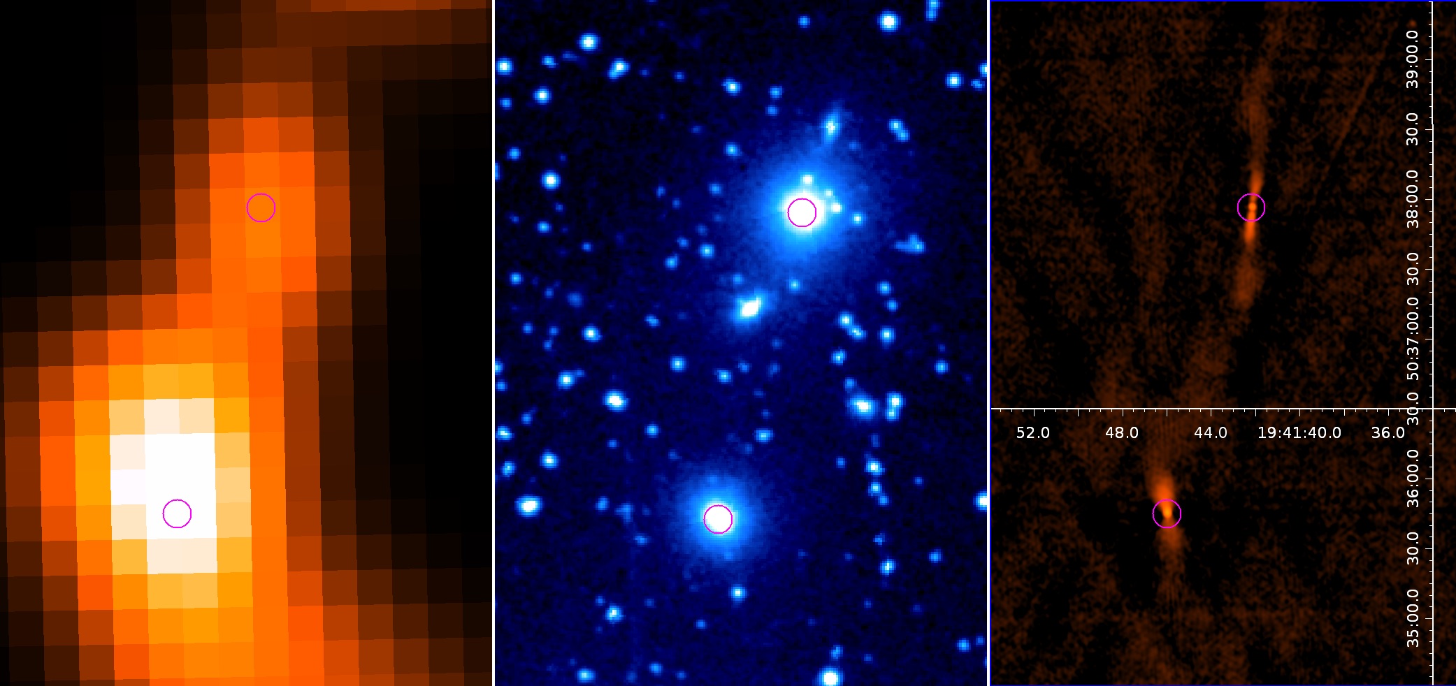
Fig. 3.5 (Left) NRAO VLA Sky Survey (NVSS); (Middle) 2nd Digitized Sky Survey Red (DSS2R*); (Right) 2017 Very Large Array Sky Survey (VLASS). Image credit: NRAO#
The strength of a radio source is measured in terms of the spectral flux density \(S(\nu)\), which is the amount of energy per second (W) per unit of frequency (Hz) per unit area (\({\rm m}^2\)). To determine the power collected by the receiver, the spectral flux must be integrated over the telescope’s collecting area and over the detector’s bandwidth (i.e., frequency interval). Mathematically the power is given as
where \(f_\nu\) is the detector efficiency at a particular frequency \(\nu\). If the detector is 100% efficient, then \(f_\nu = 1\); otherwise it is a value between 0-1. If \(S(\nu)\) is approximately constant over the bandwidth (and 100% efficient), then the integral simplifies to \(P = SA\Delta \nu\), where \(A\) is the effective area of the aperture. The unit for the spectral flux density is a jansky (Jy), where 1 Jy = \(10^{-26}\) \({\rm W}/{\rm m}^2/{\rm Hz}\). Typical measurements are on the order of mJy, where a large aperture is needed to collect enough photons to be measurable.
Exercise 3.5
The third strongest radio source in the sky is the galaxy Cygnus A, where its spectral density is 4500 Jy at 400 MHz. What is the power collected of this source over a 5 MHz frequency band with a 25 m radio telescope?
The power collected from a radio source is integrated over the frequency band observed \((\delta \nu)\) depends on the telescope’s aperature \(A\ (= 0.25 \pi D^2)\). We can calculate the power (using Eq. (3.8)) as,
assuming 100% detector efficiency, or \(f_\nu = 1\).
def radio_power(S,D_scope,freq_band):
    #S = spectral flux density (in Jy; assumed constant over the frequency band)
    #D = diameter of the telescope (in m)
    #freq_band = frequency band (in Hz)
    return (S*1e-26)*(0.25*np.pi*D_scope**2)*freq_band #returns power (in W)

source_S = 4500 #Jy
D_scope = 25 #m
delta_nu = 5*1e6 #converted to Hz

print("The power collected of the source is %1.1e W." % radio_power(source_S,D_scope,delta_nu))
The power collected of the source is 1.1e-13 W.
3.3.2. Improving Resolution: Large Apertures and Interferometry#
The resolution of a single small radio telescope poor due to Rayleigh’s criterion (Eq. (3.5)) because the wavelength \(\lambda\) is necessarily large compared to the optical regime. To obtain a comparable resolution requires a very large aperture. However, an advantage of long wavelengths is that small deviations from an ideal parabolic shape isn’t as crucial. For example, observing at 21 cm requires variations of \(\leq1\) cm (i.e., \(\lambda/20\)) in the shape of the dish to produce tolerable images.
Exercise 3.6
What diameter radio dish would be required to observe at 21 cm with a resolution equivalent to the Keck telescopes \((0.5^{\prime\prime})\)?
A telescope’s resolution depends on Rayleigh’s criterion, where we need to solve for the telescope’s aperature instead of its resolution. Rearranging Eq. (3.5), we find that
def dish_size(l,th):
    #l = lambda; wavelength in m
    #th = angular resolution; in arcseconds
    return 1.22*l/(th*np.pi/180./3600.) # returns dish size in m

l_rad = 0.21 #21 cm --> m
ang_res = 0.5 #angular resolution of Keck in arcseconds
print("A radio dish with a resolution comparable to Keck would be %2.1f km." % (dish_size(l_rad,ang_res)/1000.))
A radio dish with a resolution comparable to Keck would be 105.7 km.
For comparison, the dish at Arecibo Observatory is 305 m across and was the largest single aperture radio telescope before the construction of the Five-hundred-meter Aperture Spherical radio Telescope (FAST) in southwest China. The aperture would need to be about \(200\times\) larger to observe down to \(0.5^{\prime\prime}\).
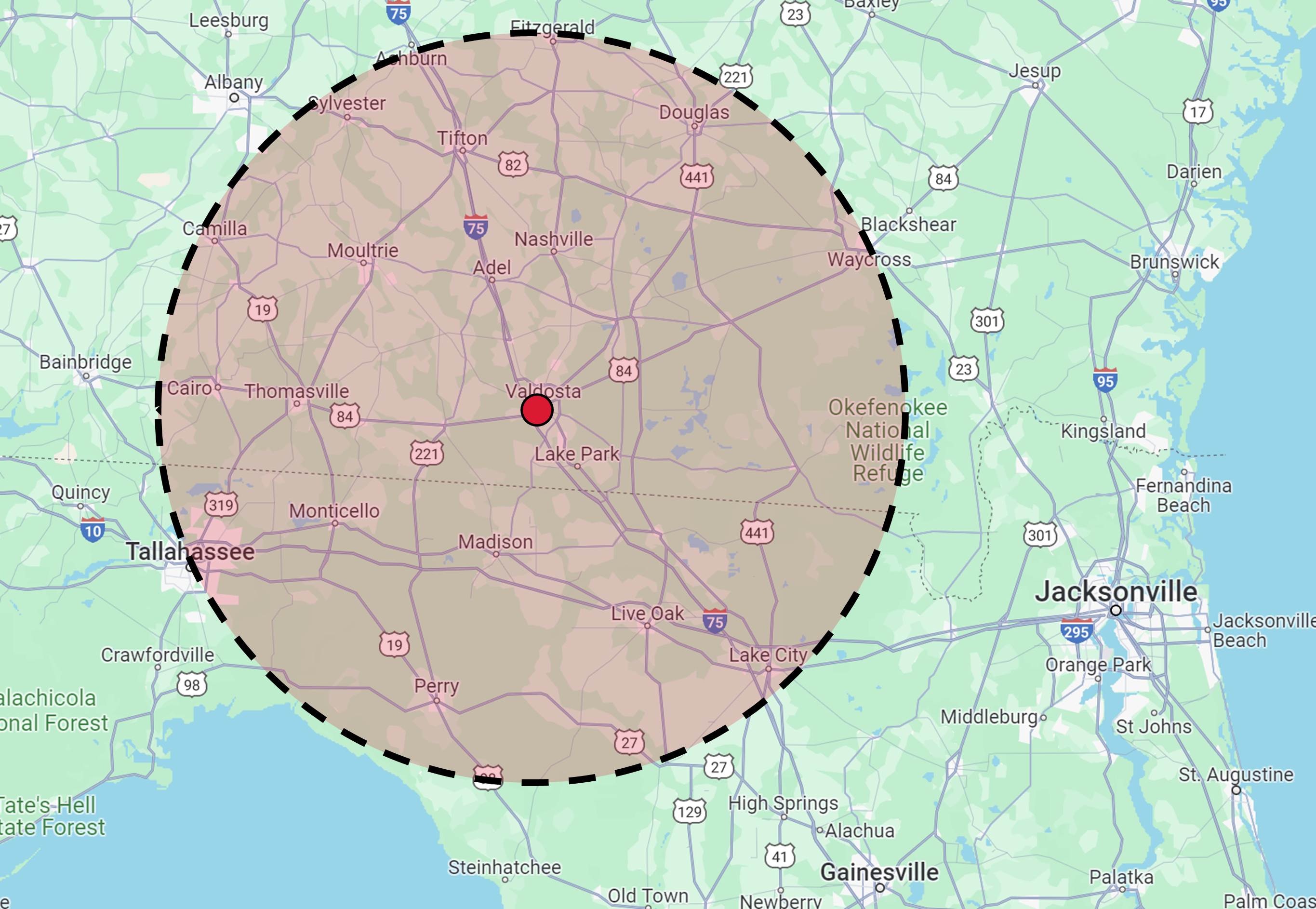
Fig. 3.6 A telescope with a single 110 km aperature would stretch from Valdosta, GA to Tallahassee, FL. Image credit: Google Maps.#
The solution to improved resolution is accomplished through a technique called interferometry, which uses multiple telescopes to mimic a larger aperture. As a result, astronomers have nevertheless been able to resolve radio images to better than \(0.001^{\prime\prime}\). For interferometry to work, astronomers utilize two radio telescopes (of modest size) separated by a baseline distance \(d\). This is similar to the Young double-slit experiment, where the baseline is analogous to the slit spacing. For the signal to arrive at both telescopes in-phase and at a maximum intensity, the extra distance traveled to one telescope must be an integral number of wavelengths \(L = n\lambda\), where \(n = 0,1,2,\ldots\). Alternatively, the signal will destructively interfere if the distance \(L = (n-1/2)\lambda\) is a odd number of half-wavelengths. The pointing angle \(\theta\) is then determined as
if the signals of the two antennas are combined and a source can be accurately located. The image resolution can be increased if two signals are received and reconstructed such that the resulting signal is coherent. Clearly, Eq. (3.9) shows this is most easily done with a longer baseline \(d\).
Very long baseline interferometry (VLBI) is possible using instruments across a whole continent or even between continents. for example, the Event Horizon Telescope (EHT) combined contemporaneous observations of M87’s galactic center to produce a direct image of a black hole’s accretion disk. It used data from radio telescopes across the world, where the exact time of data acquisition was recorded and reconstructed the image.
A single antenna has its greatest sensitivity along its pointed direction, but it can also be sensitive to radio sources at other angles. A typical antenna pattern maximizes the symmetry in dipole radiation, where there are three regions: a main lobe, back lobe and sidelobes. The longer the lobe, the more sensitive the telescope is in that direction. Note that the directionality of the beam is not perfect and components of the sidelobes contributed to a background noise. The narrowness of the main lobe is referred to as the half-power beam width (HPBW) or angular width at half its length. This width can be modulated by the addition of other telescopes to produce a particular diffraction pattern (i.e., similar to the increase in grating lines for optical diffraction) and the effect of the sidelobes can be reduced.

Fig. 3.7 Typical polar radiation plot. Most antennas show a pattern of “lobes” or maxima of radiation. In a directive antenna, shown here, the largest lobe, in the desired direction of propagation, is called the “main lobe”. The other lobes are called “sidelobes” and usually represent radiation in unwanted directions. Image credit: Wikipedia:Radiation pattern#
The Very Large Array (VLA) in Socorro, New Mexico consists of 27 radio telescopes in a movable Y configuration. The 25 m telescopes are on tracks, use receivers sensitive at a variety of frequencies, and can have a maximum configuration diameter of 27 km. It is capable of producing a high-resolution map of the sky by combining data from all of the individual telescopes. The effective collecting area is 27 times greater than a single telescope.
3.4. IR, UV, X-ray, and Gamma-ray Astronomy#
3.4.1. Atmospheric Windows in the EM Spectrum#
Optical and radio telescopes can detect a vast majority of the radiation that reaches Earth’s surface. The Earth’s atmosphere is opaque to most of the remaining electromagnetic spectrum. The primary contributor to IR absorption is water vapor, where some observatories are placed above the atmospheric water vapor to make their observations. NASA and the UK operate IR telescopes on Mauna Kea, where the humidity is quite low. The Stratospheric Observatory for Infrared Astronomy (SOFIA) uses a 2.5 m telescope mounted in a Boeing 747 with a large door in the aft fuselage and is designed for overnight flights at altitudes of about 12 km to make observations.

Fig. 3.8 Opacity of the Earth’s atmosphere as a function of wavelength. Image credit: Wikipedia:Radio window#
In addition to atmospheric absorption, IR observations are complicated by the background heat of the telescope and detector. From Wien’s law, the peak wavelength of an object near room temperature (300 K) is nearly 10 \(\mu {\rm m}\), which could be in an observer’s wavelength region of interest. Thus, steps must be taken to cool the detector to remove the signal from the background heat.
3.4.2. Observing Above the Atmosphere#
In 1983, the Infrared Astronomy Satellite (IRAS) was placed in in orbit 900 km above the Earth’s surface. It was cooled to liquid helium temperatures and its detector was sensitive to wavelengths from 12-100 \(\mu{\rm m}\). IRAS detected dust in orbit around young stars, which was an indication of the formation of planetary systems. It performed an all-sky survey in the IR, which resulted in the detection of about 350,000 sources and many of the sources (75,000) are starburst galaxies. Other new discoveries included a dust ring surrounding Vega and the first images of the Milky Way’s core.

Fig. 3.9 Nearly the entire sky, as seen in infrared wavelengths and projected at one-half degree resolution, is shown in this image, assembled from six months of data from the Infrared Astronomical Satellite (IRAS). Image credit: Wikipedia:IRAS#
From the success of IRAS, the European space Agency followed with the Infrared Space Observatory in 1995. Later, the Spitzer Space Telescope was placed into an Earth-trailing orbit in 2003 and was recently retired in 2020. The mission was only planned to last 2.5 years. The liquid helium was exhausted in 2009 and the telescope was repurposed to continue observing in its Warm Mission, which limited its observations to 3.6 and 4.5 \(\mu{\rm m}\). Spitzer had a 0.85 m (f/12) mirror constructed of beryllium and was cooled to less than 5.5 K prior to 2009.

Fig. 3.10 The Andromeda Galaxy imaged by the MIPS instrument at 24 μm using the Spitzer Space Telescope. Image credit: Wikipedia:Spitzer_Space_Telescope#
The Cosmic Background Explorer (COBE) was launched and operated from 1989-1993 investigating the microwave regime. It measured the microwave background radiation as 2.7 K, which validated the previous measurements made from the ground. COBE was followed by two more advanced spacecraft: the Wilkinson Microwave Anisotropy Probe (WMAP) operated from 2001 to 2010 and the Planck spacecraft from 2009 to 2013
Shorter wavelengths require a very precise reflecting surface and it wasn’t until the Space Age could UV, X-ray, or Gamma-ray observations could be performed. The International Ultraviolet Explorer (IUE) was operated from 1978-1996 and proved to be a remarkably productive instrument. The most famous X-ray telescope Chandra has been in operation from 1999 and operates from 6.2 - 0.1 nm (0.2 - 10 keV) with an angular resolution of approximately \(0.5^{\prime\prime}\). Because X-rays cannot be focused in the same way that longer wavelengths can, grazing incidence mirrors are used to achieve the outstanding resolving power of Chandra.
The Compton Gamma Ray Observatory (CGRO) was a space observatory designed to detect radiation with energy from 20 keV to 30 GeV. The observatory was in operation from Earth orbit from 1991-2000 and housed four main telescopes that completed the first all sky survey for energies above 100 MeV. Successors to CGRO include the ESA INTEGRAL spacecraft (launched 2002), NASA’s Swift Gamma-Ray Burst Mission (launched 2004), ASI AGILE (launched 2007) and NASA’s Fermi Gamma-ray Space Telescope (launched 2008); all remain operational as of 2019.
3.5. Homework#
Problem 1
The diffraction pattern for a single slit is given by
where \(\beta = 2\pi D\sin(\theta)/\lambda\).
(a) Plot \(I/I_o\) vs \(m\) over the range {-3,3}. Hint: Single slit diffraction has a relation that can relate \(\beta\) to \(m\), but \(m\) is treated as float for the plotting.
(b) If the slit has an aperture of 1.0 \(\mu m\), what angle \(\theta\) (in deg.) corresponds to the first minimum if the wavelength of light is 500 nm?
Problem 2
Using the Rayleigh criterion, estimate the angular resolution limit of the human eye at 440 nm. Assume the pupil diameter is 5 mm.
Problem 3
A refracting astronomical telescope has a magnifying power of 150 when adjusted for minimum eyestrain. Its eyepiece has a focal length of +1.20 cm. Determine the focal length of the objective lens.
Problem 4
The large telescope at Mt Palomar has a concave objective mirror diameter of 5.0 m and radius of curvature 46 m. What is the magnifying power of the instrument when it is used with an eyepiece of focal length 1.25 cm?
Problem 5
What would the diameter of a single radio dish need to be to have a collecting area equivalent to the 27 telescopes of the VLA?
Problem 6
How much must the pointing angle of a two-element radio interferometer be changed in order to move from one interference maximum to the next? Assume that the two telescopes are separated by the diameter of Earth and that the observation is being made at a wavelength of 21 cm. Express your answer in arcseconds.