12. The Degenerate Remnants of Stars#
12.1. The Discovery of Sirius B#
In 1838, Friedrich Wilhelm Bessel used the technique of stellar parallax to find the distance to the star 61 Cygni. The next candidate Bessel tried was Sirius, the brightest star in the sky. It’s parallax angle is \(p = 0.379^{\prime\prime}\), which corresponds to a distance of only 2.64 pc, or 8.61 ly. Sirius’ brilliance is due (in part) to its proximity to Earth. Bessel tracked Sirius’ path across the sky and found that it deviated slightly from a straight line. Using 10 years of precise observation, Bessel concluded (in 1844) that Sirius was actually a binary star system. He deduced that the binary orbital period was 50 years, where the modern value is \(50.1284 \pm 0.0043\) years (Bond et al 2017) and the position of the secondary star.

Fig. 12.1 The white dwarf, Sirius B, next to the overexposed image of Sirius A. Image Credit: Wikipedia:Sirius; NASA, ESA, H. Bond (STScI), and M. Barstow (University of Leicester)#
Bessel’s telescopes were incapable of finding the “Pup” (i.e., the unseen companion of the luminous “Dog Star”) due to the glare of Sirius. After Bessel’s death in 1846, the search for the Pup waned. In 1862, Alvan Graham Clark tested his father’s new 18-inch refractor (3 inches longer than any previous instrument) on Sirius, and he discovered the Pup at its predicted position. The dominant Sirius A was measured to be nearly \(1000\times\) brighter than the Pup (now called Sirius B). The orbits of the stars about their center of mass revealed that Sirius A and Sirius B are about \(2.3\ M_\odot\) and \(1.0\ M_\odot\), respectively. The modern values are \(2.063 \pm 0.023\ M_\odot\) and \(1.018 \pm 0.011\ M_\odot\) (Bond et al 2017).

Fig. 12.2 The orbits of Sirius A and Sirius B. Image Credit: Wikipedia:Sirius#
Clark’s discovery of Sirius B was made when the stars were most widely separated (by just \(10^{\prime\prime}\)) at apastron. The great difference in their luminosities: \(L_A = 25.4\ L_\odot\) and \(L_B=0.056\ L_\odot\) makes observations difficult when the stars are closer together on the sky. The next apastron comes 50 years later, where spectroscopists developed the tools to measure each star’s surface temperature. From the Pup’s faint appearance, astronomers expected it to be cool and red, but they discovered that it is a hot, blue-white star that emits much of its energy in the UV. Modern observations measure the surface temperature of Sirius B (the Pup) at \(25,000 \pm 200\ {\rm K}\), which is much hotter than Sirius A at \(9940\ {\rm K}\).
Exercise 12.1
Given the modern measurements, what is the size and density of Sirius B?
The size of Sirius B can be estimated using the Stefan-Boltzman law,
where the Sun’s surface temperature is \(5777\ {\rm K}\). Rearranging the above equation in terms of the stellar radius \(R\), we get
The size of Sirius B is 0.0126 \(R_\odot\) or 1.38 \(R_\oplus\), while the density is \(7.11 \times 10^8\ {\rm kg/m^3}\). Sirius B is a Solar mass star compressed into a roughly Earth-sized volume and the acceleration due to gravity is about \(1.8 \times 10^6\ {\rm m/s^2}\).
import numpy as np
from scipy.constants import G

L_SiriusB = 0.056 #luminosity in solar units
T_SiriusB = 25000 #surface temperature of Sirius B in K
T_sun = 5777 #surface temperature of the Sun in K
R_sun = 6.957e8 #radius of the Sun in m
R_Earth = 6371e3 #radius of the Earth in m

R_SiriusB = np.sqrt(L_SiriusB)*(T_sun/T_SiriusB)**2

print("The radius of Sirius B is %1.4f R_Sun, %1.2f R_Earth, or %1.2e m." % (R_SiriusB,R_SiriusB*R_sun/R_Earth,R_SiriusB*R_sun))

M_sun = 1.989e30 #mass of the Sun in kg
M_SiriusB = 1.018 #mass of Sirius B in solar units

rho_SiriusB = (M_SiriusB*M_sun)/(4./3.*np.pi*(R_SiriusB*R_sun)**3)
print("The density of Sirius B is %1.2e kg/m^3" % rho_SiriusB)

g_SiriusB = G*M_SiriusB*M_sun/(R_SiriusB*R_sun)**2
print("The acceleration due to gravity at the surface of Sirius B is %1.2e m/s^2." % g_SiriusB)
The radius of Sirius B is 0.0126 R_Sun, 1.38 R_Earth, or 8.79e+06 m.
The density of Sirius B is 7.11e+08 kg/m^3
The acceleration due to gravity at the surface of Sirius B is 1.75e+06 m/s^2.
On Earth, the pull of gravity on a teaspoon of white dwarf material would be approximately \(34,300\ {\rm N}\). This fierce gravity reveals itself in the spectrum of Sirius B, where it produces an immense pressure near the surface that results in very broad hydrogen absorption lines. Apart from these lines, its spectrum is a featureless continuum.
Astronomers initially dismissed the results, calling them “absurd”. However, the calculations are so simple and straightforward that this attitude changed. In 1922, Eddington said, “Strange objects, which persist in showing a type of spectrum entirely out of keeping with their luminosity, may ultimately teach us more than a host which radiate according to rule.” Like all sciences, astronomy advances most rapidly when confronted with exceptions to its theories.
12.2. White Dwarfs#
Obviously Sirius B is not a normal star, where it is in a class of stars that have approximately the mass of the Sun and the size of Earth called white dwarfs. As many as 1/4 of the stars in the Solar neighborhood may be white dwarfs. The average characteristics of these faint stars have been difficult to determine because a complete sample has only been obtained within 10 pc of the Sun.
12.2.1. Classes of White Dwarf Stars#
White dwarfs occupy a narrow sliver of the H-R diagram that is roughly parallel to (and below) the main sequence. Although white dwarfs are typically whiter than normal stars, the name itself is a misnomer since they come in all colors, with surface temperatures ranging from \(5000-80,000\ {\rm K}\). Their spectral type D has several subdivisions,
the largest group (about 2/3 of the total number, including Sirius B) is called DA white dwarfs and display only pressure-broadened hydrogen absorption lines in their spectra.
Hydrogen lines are absent from the DB white dwarfs (8% of the total number), which show only helium absorption lines.
No lines are shown at all in the DC white dwarfs (14% of the total number), only a continuum devoid of features.
The remaining 11% include the DQ white dwarfs that exhibit carbon features in their spectra and DZ white dwarfs that have evidence of metal lines.
12.2.2. Central Conditions in White Dwarfs#
White dwarfs are very massive for their size, where we can not estimate the central pressure and temperature using our derived values. Assuming that Sirius B represents a typical white dwarf (at least 2/3 of them) and recalling the estimate for the central pressure from hydrostatic equilibrium, we have
which is roughly \(5.5 \times 10^{21}\ {\rm N/m^2}\) or 200,000 times greater than the pressure in the Sun \((P_{c,\odot} = 2.477 \times 10^{16}\ {\rm N/m^2})\).
import numpy as np
from scipy.constants import G

M_sun = 1.989e30 #mass of the Sun in kg
T_sun = 5777 #surface temperature of the Sun in K
R_sun = 6.957e8 #radius of the Sun in m

M_SiriusB = 1.018*M_sun #mass of Sirius B in kg
L_SiriusB = 0.056 #luminosity in solar units
T_SiriusB = 25000 #surface temperature of Sirius B in K

R_SiriusB = np.sqrt(L_SiriusB)*(T_sun/T_SiriusB)**2*R_sun #radius of Sirius B in m

rho_SiriusB = M_SiriusB/(4./3.*np.pi*R_SiriusB**3)

P_c = (2./3.)*G*np.pi*rho_SiriusB**2*R_SiriusB**2
print("The central pressure in Sirius B is %1.2e N/m^2." % P_c)

P_sun = 2.477e+16 #central pressure in Sun in N/m^2
print("The central pressure in Sirius B is %1.0e times greater than the Sun." % (P_c/P_sun))
The central pressure in Sirius B is 5.47e+21 N/m^2.
The central pressure in Sirius B is 2e+05 times greater than the Sun.
A crude estimate of the central temperature can be obtained for the radiative temperature gradient as
assuming that the surface temperature \(T_{wd} \ll T_c\). We can also assume that \(\overline{\kappa} = 0.02\ {\rm m^2/kg}\) (from the Rosseland mean opacity for electron scattering with \(X=0\)), which gives
import numpy as np
from scipy.constants import G,sigma,c

M_sun = 1.989e30 #mass of the Sun in kg
T_sun = 5777 #surface temperature of the Sun in K
R_sun = 6.957e8 #radius of the Sun in m
L_sun = 3.827e26 #luminosity of the Sun in W

M_SiriusB = 1.018*M_sun #mass of Sirius B in kg
L_SiriusB = 0.056*L_sun #luminosity in solar units
T_SiriusB = 25000 #surface temperature of Sirius B in K

R_SiriusB = np.sqrt(L_SiriusB/L_sun)*(T_sun/T_SiriusB)**2*R_sun #radius of Sirius B in m
rho_SiriusB = M_SiriusB/(4./3.*np.pi*R_SiriusB**3)
kappa_es = 0.02
a_rad = 4.*sigma/c

T_c = ((3*kappa_es*rho_SiriusB/(4*a_rad*c))*(L_SiriusB/(4.*np.pi*R_SiriusB)))**0.25

print("The central temperature in Sirius B is %1.2e K." % T_c)
The central temperature in Sirius B is 5.50e+07 K.
These estimated values for a white dwarf show that hydrogen must be absent from the subsurface layers because they are high enough to start fusion and the white dwarf luminosities would be several orders of magnitude larger than observed. As a result, the interiors of white dwarfs must contain particles that are incapable of fusion at these densities and temperatures (e.g., constituents of the PP I chain).
White dwarfs are born from the cores of low- and intermediate-mass stars (i.e., those with a ZAMS mass \(\lesssim 8-9\ M_\odot\)) near the end of their lives on the AGB of the H-R diagram. Any star with a helium core mass \(\gtrsim 0.5\ M_\odot\) will undergo fusion and thus, most white dwarfs consist primarily of completely ionized carbon and oxygen nuclei (i.e., the left over \({\rm CO}\) core). As an AGB star ages, it expels its surface layers as planetary nebula, which exposes the core as a white dwarf. The distribution of DA white dwarf masses is sharply peaked at \(0.56\ M_\odot\), with some 80% lying between \(0.42-0.70\ M_\odot\). The much larger main-sequence masses must be lost on the AGB through thermal pulses and a superwind.

Fig. 12.3 DA white dwarfs on an H-R diagram. A line marks the location of the \(0.5\ M_\odot\) white dwarfs and a portion of the main sequence is at the upper right. (Carroll & Ostlie (2007); Data from Bergeron, Saffer, and Liebert, Ap. J., 394, 228, 1992)#
12.2.3. Spectra and Surface Composition#
The exceptionally strong pull of a white dwarf’s gravity is responsible for the characteristic spectrum of DA white dwarfs. In this process, heavier nuclei are pulled below the surface while the lighter hydrogen rises to the top and results in a thin outer layer of hydrogen covering a helium layer on top of the \({\rm CO}\) core. This vertical stratification takes only \(\sim100\) years in the hot stellar atmosphere.
The origin of the non-DA (e.g., DB and DC) white dwarfs is not yet clear. Efficient mass-loss may occur on the AGB associated with the thermal pulse or superwind phases, which strip the white dwarf of nearly all of its hydrogen. Alternatively, a single white dwarf may be transformed between the DA and non-DA spectral types through convective mixing. For example, the helium convection zone’s penetration into a thin hydrogen layer could change a DA into a DB white dwarf by diluting the hydrogen with additional helium.
12.2.4. Pulsating White Dwarfs#
White dwarfs with surface temperatures of \(T_e \approx 12,000\ {\rm K}\) lie within the instability strip of the H-R diagram and pulsate with periods between \(100-1000\ {\rm s}\). In 1968, Arlo Landolt discovered a class of variable white dwarf stars, which are known as ZZ Ceti variables or DAV stars. The pulsation periods correspond to the nonradial g-modes that resonate within the white dwarf’s surface layers of hydrogen and helium. These g-modes involve almost perfectly horizontal displacement and thus, the radii of these compact pulsators hardly change. Their brightness variations (\(\sim 0.1\ {\rm mag}\)) are due to temperature variations on the stellar surface.
Successful numerical calculations of pulsating white dwarf models were carried out by Don Winget (and others), where they demonstrated that the hydrogen partial ionization zone is responsible for driving oscillations in the ZZ Ceti stars. These computations also confirmed the elemental stratification of white dwarf envelopes. These numerical models predict that hotter DB white dwarfs should also exhibit g-mode oscillations driven by the helium partial ionization zone. Within a year’s time from the initial prediction, it was confirmed when the first DBV star was discovered. Some stars are described by their transition to the white dwarf stage as: DOV and PNNVs stars that have an effective temperature \(T_e \approx 10^5\ {\rm K}\). The DO spectral type marks the initial stage of the white dwarf and the PNNV stands for planetary nebula nuclei.

Fig. 12.4 Compact pulsators on the H-R diagram. (Carroll & Ostlie (2007); Figure adapted from Winget, Advances in Helio- and Asteroseismology, Christensen-Dalsgaard and Frandsen (eds.), Reidel, Dordrecht, 1988)#
12.3. The Physics of Degenerate Matter#
12.3.1. The Pauli Exclusion Principle and Electron Degeneracy#
Any system consists of quantum states that are identified by a set of quantum numbers. A box of gas particles is filled with standing de Broglie waves that are described by three quantum numbers specifying a particle’s momentum in each of three directions. If the gas particles are fermions (e.g., electrons or neutrons), then the Pauli exclusion principle allows at most one fermion in each quantum state because no two fermions can have the same set of quantum numbers.
At standard temperature and pressure (\(20\ {\rm ^\circ C}\) and 101,325 \({\rm N/m^2}\)), only one of every \(10^7\) quantum states is occupied by a gas particle, and the limitations imposed by the Pauli exclusion principle become insignificant. Ordinary gas has a thermal pressure that is related to it temperature by the ideal gas law (i.e., \(PV = NkT\)). As energy (\(PV\)) is removed from the gas and its temperature falls, an increasingly large fraction of the particles are forced into lower energy states. If the particles are fermions, only one particle is allowed in each state and thus, all the particles cannot crowd into the ground state.
As the temperature of the gas is lowered, the fermions will fill up the lowest available unoccupied state first and successively occupy the excited states with the lowest energy. Even in as the temperature approaches absolute zero (\(T\rightarrow 0\ {\rm K}\)), the motion of the fermions in excited states produces a gas pressure. At absolute zero, all the lower energy states and none of the higher energy states are occupied. In this case, the fermion gas is completely degenerate.
12.3.2. The Fermi Energy#
The maximum energy of any electron in a completely degenerate gas (at absolute zero) is known as the Fermi energy \(\varepsilon_F\). To determine this limiting energy, consider a 3D box of length L on each side. Treating the electrons as standing waves in the box, their wavelengths in each dimension are,
where there are integer quantum numbers (\(N_x\), \(N_y\), and \(N_z\)) associated with each dimension. Recalling that the de Broglie wavelength is related to the components of momentum by,

Fig. 12.5 Fraction of states of energy \(\varepsilon\) occupied by fermions. For \(T=0\), all fermions have \(\varepsilon \leq \varepsilon_F\), but for \(T>0\), some fermoins have energies in excess of the Fermi energy. (Carroll & Ostlie (2007))#
The total kinetic energy of a particle is the sum of the squares of each component of the momentum, or
In terms of all the fundamental constants, the energy is
The total number of electrons in the gas corresponds to the total number of unique quantum numbers \((N_x,\ N_y,\ \text{and}\ N_z)\) times two.
Note
The factor two arises due to the electrons being spin \(1/2\) particles, so \(m_s \pm 1/2\) implies that two electron can have the same combination of \(N_x,\ N_y,\ \text{and}\ N_z\), while still maintaining a unique set of four quantum numbers.
Each integer in a coordinate N-space corresponds to the quantum state of two electrons. With a large enough sample of electrons, the electrons will fill out up to a radius \(N\) but only for the positive octant of N-space (i.e., \(N_x>0\), \(N_y>0\), and \(N_z>0\)). this means that the total number of electrons will be
Solving for \(N\) and substituting into Eq. (12.2), we find that the Fermi energy is given by
which depends on the mass of the electron \(m_e\) and the number of electrons per unit volume \((n \equiv N_e/L^3)\). The average energy per electron at absolute zero is \(\frac{3}{5}\varepsilon_F\). The above derivation applies to any fermion, not just electrons.
12.3.3. The Condition for Degeneracy#
Some of the states with an energy less than \(\varepsilon_F\) will become vacant as fermions use their thermal energy to occupy more energetic states. Although the degeneracy will not be precisely complete when \(T>0\ {\rm K}\), the assumption of complete degeneracy is a good approximation at the densities encountered in the interior of a white dwarf. All but the most energetic particles will have an energy less than the Fermi energy
To understand the dependency of degeneracy on both temperature and density, we express the Fermi energy in terms of the density of the electron gas. For full ionization, the number of electrons per unit volume is
which depends on the number of protons \(Z\), nucleons \(A\), and the mass of the hydrogen atom \(m_H\). The Fermi energy is proportional to the \(2/3\) power of the density,
Compare the Fermi energy with the average thermal energy of an electron (\(\frac{3}{2}kT\)). In rough terms, if \(\frac{3}{2}kT < \varepsilon_F\), then an average electron wil be unable to make a transition to an unoccupied state, and the electron will be degenerate. For a degenerate gas,
or
For \(Z/A = 0.5\), the right-hand side is \(\mathcal{D} \equiv 1261\ {\rm K\ m^2/kg^{2/3}}\), so that the condition for degeneracy can be written as
The smaller the value of \(T/\rho^{2/3}\), the more degenerate the gas.
Exercise 12.2
How important is electron degeneracy at the centers of the Sun and Sirius B?
At the center of the standard solar model, \(T_c = 1.57 \times 10^7\ {\rm K}\) and \(\rho_c = 1.527 \times 10^5\ {\rm kg/m^3}\). Then
In the Sun, electron degeneracy is quite weak and plays a very minor role supplying only \(\sim 0.1\%\) of the central pressure. However, as the Sun continues to evolve, electron degeneracy will become increasingly important.
For Sirius B, the values of the density and central temperature estimated above lead to
which validates the assumption of complete degeneracy for Sirius B.
import numpy as np
from scipy.constants import G,sigma,c

rho_sun_c = 1.527e5 #central density of the Sun in kg/m^3
T_sun_c = 1.57e7 #central temperature fo the Sun in K
degen_sun = T_sun_c/rho_sun_c**(2/3)

rho_SiriusB_c = 7.11e8 #central density of Sirius B in kg/m^3
T_SiriusB_c = 5.50e7 # central temperature for Sirius B in K
degen_SiriusB = T_SiriusB_c/rho_SiriusB_c**(2/3)

print("The condition for degeneracy is %d K m^2/kg^{2/3} for the Sun." % degen_sun)
print("The condition for degeneracy is %d K m^2/kg^{2/3} for Sirius B." % degen_SiriusB)
The condition for degeneracy is 5495 K m^2/kg^{2/3} for the Sun.
The condition for degeneracy is 69 K m^2/kg^{2/3} for Sirius B.

Fig. 12.6 Degeneracy in the Sun’s center as it evolves. (Carroll & Ostlie (2007); Data from Mazzitelli and D’Antona, Ap. J., 311, 762, 1986)#
12.3.4. Electron Degeneracy Pressure#
We can estimate the electron degeneracy pressure by combining two key ideas of quantum mechanics:
The Pauli exclusion principle, which allows at most one electron in each quantum state, and
Heisenberg’s uncertainty principle in the form of, \(\Delta x\ \Delta p_x \approx \hbar\), which requires that an electron confined to small volume of space have a correspondingly high uncertainty in its momentum.
When we make the unrealistic assumption that all of the electrons have the same momentum \(p\), the pressure integral becomes
which depends on the total electron number density \(n_e\) and average speed \(v\) of the electrons.
In a completely degenerate electron gas and for a uniform number density of \(n_e\), the separation between neighboring electrons is about \(n_e^{-1/3}\). However, the electron must maintain their identities as different particles to satisfy the Pauli exclusion principle (i.e., the uncertainty in their positions cannot be larger than their physical separation). Identifying \(\Delta x \approx n_e^{-1/3}\) for the limiting case of complete degeneracy, we can use Heisenberg’s uncertainty relation to estimate the momentum of an electron. In on coordinate direction,
In a 3D gas each of the directions is equally likely, which implies that
and is just a statement of the equipartition of energy among all the coordinate directions. Therefore,
or
Using Eq. (12.4) for the electron number density with full ionization gives
For nonrelativistic electrons, the speed is
Inserting Eqs. (12.4) and (12.8) into Eq. (12.9) for for the electron degeneracy pressure results in
This is roughly a factor of two smaller than the exact expression for the pressure due to a completely degenerate, nonrelativistic electron gas \(P\),
Using \(Z/A = 0.5\) for a carbon-oxygen white dwarf, Eq. (12.11) shows that the electron degeneracy pressure available to support Sirius B is about \(1.9 \times 10^{22}\ {\rm N/m^2}\), which is within a factor of two from the central pressure estimated in Eq. (12.1). Electron degeneracy pressure is responsible for maintaining the hydrostatic equilibrium in a white dwarf.
Note
You may have noticed that Eq. (12.11) is the polytropic equation of state, \(P=K\rho^{5/3}\) with the polytropic index \(n = 3/2\). This implies that the Lane-Emden equation can be used to study these objects.
12.4. The Chandrasekhar Limit#
12.4.1. The Mass-Volume Relation#
The relation between the radius \(R_{wd}\) and mass \(M_{wd}\) of a white dwarf can be found by setting the estimate of the central pressure (Eq. (12.1)) equal to the electron degeneracy pressure (Eq. (12.11)):
Assuming a constant density for the white dwarfs leads to an estimate of the radius,
For a Solar-mass carbon-oxygen white dwarf, \(R_{wd} \approx 2.9 \times 10^6\ {\rm m}\), which is too small by roughly a factor of 2 but an acceptable estimate. A surprising implication is that \(M_{wd}R_{wd}^3 = \text{constant}\), or
The volume of a white dwarf is inversely proportional to its mass, where more massive white dwarfs are actually smaller. This mass-volume relation is a result of the electron degeneracy pressure supporting the star. The electrons must be more closely confined to generate the larger degeneracy pressure required to support a more massive star (i.e., \(\rho \propto M_{wd}^2\)).
According to the mass-volume relation, a white dwarf would eventually shrink down to zero volume in the limit of continually adding mass. However, if the density exceeds about \(10^9\ {\rm kg/m^3}\), then there is a departure from this relation. Using Eq. (12.9) to estimate the speed of electrons in Sirius B results in
which is \(0.23c\).
from scipy.constants import hbar, m_e,c

Z = 1.
A = 2.
m_H = 1.6735575e-27 #mass of hydrogen in kg
rho_SiriusB = 7.11e8 #central density of Sirius B in kg/m^3

v_e =(hbar/m_e)*((Z/A)*(rho_SiriusB/m_H))**(1./3.)
print("The average speed of electrons in Sirius B is %1.2e m/s or %1.3f c." % (v_e,v_e/c))
The average speed of electrons in Sirius B is 6.91e+07 m/s or 0.230 c.
If the mass-volume relation were correct, white dwarfs a bit more massive than Sirius B would be so mall and dense that their electrons would be superluminal (i.e., faster than the speed of light). This points to the dangers of ignoring relativity in our expressions for the electron speed and pressure. Because the electrons are moving more slowly than the nonrelativistic Eq. (12.10) would indicate, there is less electron pressure available to support the star. Thus, a massive white dwarf is smaller than predicted by the mass-volume relation. There is a limit to the amount of matter than can be supported by electron degeneracy pressure.
12.4.2. Dynamical Instability#
To appreciate the effect of relativity on the stability of a white dwarf, recall that Eq. (12.11) is a polytropic equation (\(P = K\rho^{5/3}\)). The ratio of the specific heats \(\gamma = 5/3\) in the nonrelativistic limit. This means that the white dwarf is dynamically stable. If it suffers a small perturbation, then it will return to its equilibrium structure instead of collapsing. In the extreme relativistic limit, the electron speed \(v=c\) must be used to find the degeneracy pressure, which results in
In this limit, \(\gamma = 4/3\) corresponds to dynamical instability and introduces a polytropic equation with an index \(n=3\). The smallest departure from equilibrium will cause the white dwarf to collapse as the electron degeneracy pressure fails. Approaching this limiting case leads to the collapse of the degenerate core in an aging supergiant and results in a core-collapse supernova.
12.4.3. Estimating the Chandrasekhar Limit#
An approximate value for the maximum white dwarf mass can be obtained by setting Eq. (12.14) equal to the estimate of the central pressure (Eq. (12.1)) to get
and solving for \(\rho\) to get,
Using \(\rho = M_{wd}/\frac{4}{3}\pi R_{wd}^3\) gives
and
Using \(Z/A = 0.5\) results in \(0.44\ M_\odot\) for the greatest possible mass. Note that Eq. (12.15) contains the fundamental constants \(\hbar\), \(c\), and \(G\), which represent the combined effects of quantum mechanics relativity, and Newtonian gravitation on the structure of a white dwarf. A precise derivation with the Lane-Emden equation results in a value of \(M_{Ch} \approx 1.4\ M_\odot\), which is the Chandrasekhar limit.
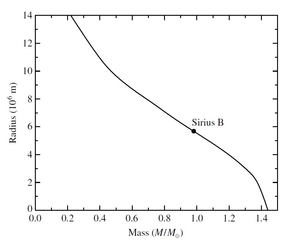
Fig. 12.7 Radii of white dwarfs of \(M_{wd}\leq M_{Ch}\) at \(T = 0\ {\rm K}\). (Carroll & Ostlie (2007))#
It is important to emphasize that the gas pressure of the ideal gas law and the expression for radiation pressure depend explicitly on temperature, where the pressure of a completely degenerate electron gas is independent of its temperature. This has the effect of decoupling the mechanical structure of the star from its thermal properties.
12.5. The Cooling of White Dwarfs#
Most stars end their lives as white dwarfs, where no fusion occurs in their interiors. White dwarfs simply cool off at an essentially constant radius as they slowly deplete their supply of thermal energy. Just as paleontologists can read the history of Earth’s life in the fossil record, astronomers try to recover the history of star formation by studying the statistics of white-dwarf temperatures.
12.5.1. Energy Transport#
“How is energy transported outward from the interior of a white dwarf?” In an ordinary star, photons travel much farther than atoms do before a collision that robs them of energy. As a result, photons are normally more efficient carriers of energy to the stellar surface. In a white dwarf, the degenerate electrons can travel long distances before losing energy in a collision with a nucleus because the vast majority of the lower-energy electron states are already occupied. Thus, energy is carried by electron conduction rather than by radiation.
This process is so efficient that hte interior of a white dwarf is nearly isothermal, with the temperature dropping significantly only in the nondegenerate surface layers. The steep temperature gradient near the surface creates convection zones that may alter the appearance of the white dwarf’s spectrum as it cools.
At the surface, a white dwarf has a luminosity \(L_{wd}\) and mass \(M_{wd}\) that contribute to a surface pressure \(P\) as a function of the temperature because the envelope is nondegenerate. The equation for this surface pressure is
which depends on the coefficient of the bound-free Kramers opacity law
Using the ideal gas law to replace the pressure results in a relation between the density and temperature,
The transition between the nondegenerate surface layers of the star and its isothermal degenerate interior of temperature \(T_c\) is described by substituting Eq. (12.17) in Eq. (12.6) by finding
and substituting into \(\mathcal{D} = T/\rho^{2/3}\) and solving \(L_{wd}\) by
where
Note that the luminosity is proportional to the interior temperature \(T_c^{7/2}\) and that is varies to the fourth power of the effective temperature according to the Stefan-Boltzmann law. Thus, the surface of a white dwarf cools more slowly than its isothermal interior as the star’s thermal energy leaks into space (i.e., \(\frac{7}{2} < 4\)).
Exercise 12.3
What is the interior temperature of a Solar-mass white dwarf with \(L_{wd} =0.03 L_\odot\)? Assume that \(X = 0,\ Y=0.9,\ \text{and}\ Z=0.1\) for the nondegenerate envelope so \(\mu \simeq 1.4\).
Using Eq. (12.18) and solving for \(T_c\), we get
Substituting into the equation for the degeneracy condition shows that the density at the base of the nondegenerate envelope is about
This result is several orders of magnitude less than the average density of a Solar-mass white dwarf (e.g., Sirius B). It also confirms that the envelope is indeed thin and contributes very little to the star’s total mass.
L_sun = 3.827e26 #luminosity of the Sun in W
L_wd = 0.03*L_sun #Luminosity of the white dwarf in W
M_wd = 1. #Solar-mass white dwarf

Z = 0.1
X = 0
mu = 1.4

T_c = ((L_wd/6.65e-3)*(1./M_wd)*(Z*(1+X)/mu))**(2/7)
print("The interior temperature of the white dwarf is %1.2e K." % T_c)

D = 1261 # degeneracy condition in K m^2/kg^(2/3)
rho = (T_c/D)**1.5

print("The density at the base of the nondegenerate envelope is %1.2e kg/m^3." % rho)
The interior temperature of the white dwarf is 2.85e+07 K.
The density at the base of the nondegenerate envelope is 3.39e+06 kg/m^3.
12.5.2. The Cooling Timescale#
A white dwarf’s thermal energy primarily resides in this kinetic energy of its nuclei, where the degenerate electrons cannot give up a significant amount of energy nearly all the lower energy state are already occupied. If we assume for simplicity that the composition is uniform, then the total number of nuclei in the white dwarf is equal to the star’s mass \(M_{wd}\) divided by the mass of a nucleus \(Am_H\). Since the average thermal energy of a nucleus is \(\frac{3}{2}kT\), the thermal energy available for radiation is
If use \(T_c = 2.8\times 10^7\ {\rm K}\) and \(A = 12\) for carbon, then Eq. (12.19) gives approximately \(6 \times 10^{40}\ {\rm J}\). A crude estimate of the characteristic timescale for cooling \(\tau_{cool}\) can be made simply by dividing the thermal energy by the luminosity. Thus
which is about \(5.2 \times 10^{15}\ {\rm s} \approx 170\ {\rm Myr}\). This is an underestimate, because the cooling timescale increases as \(T_c\) decreases.
12.5.3. The Change in Luminosity with Time#
The depletion of the internal energy provides the luminosity, so Eqs. (12.18) and (12.19) give
or
If the initial temperature of the interior is \(T_o\), then this expression may be integrated to obtain the core temperature as a function of time:
where the timescale for cooling at the initial temperature is \(\tau_o \equiv \frac{3M_{wd}k}{2Am_H C T_o^{5/2}}\). Using the same logic for Eq. (12.18) shows that the luminosity of the white dwarf declines sharply from its initial value \((L_o = C T_o^{7/2})\) and then dims much more gradually as time passes:
12.5.4. Crystallization#
As a white dwarf cools, it crystallizes in a gradual inside-out process. An upturned “knee” occurs in theoretical cooling curves at about \(L_{wd}/L_\odot \approx 10^{-4}\) when the cooling nuclei begin settling into a crystalline lattice. The regular crystal structure is maintained by the mutual electrostatic repulsion of the nuclei, where it minimizes their energy as they vibrate about their average position in the lattice.
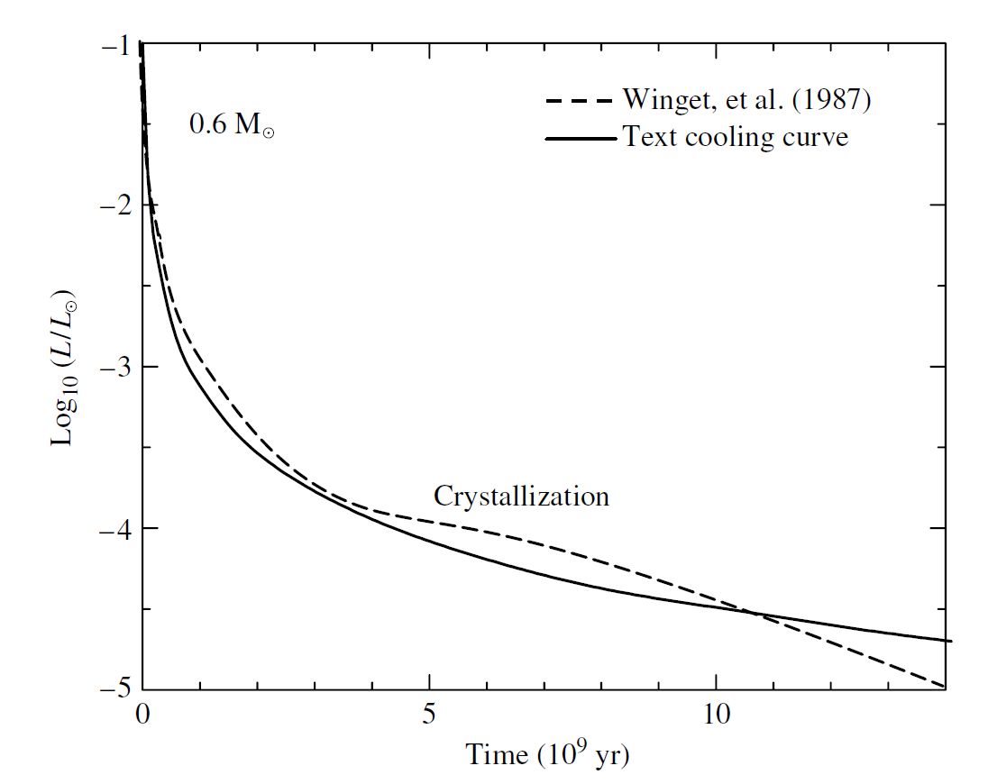
Fig. 12.8 Theoretical cooling curves for \(0.6\ M_\odot\) white dwarf models. The solid line is from Eq. (12.22), and the dashed line is from Winget et al. (1987) (Carroll & Ostlie (2007))#
As the nuclei undergo this phase change, they release their latent heat (about \(kT\) per nucleus), which slows the star’s cooling and produces the knee in the cooling curve. Later as the white dwarf’s temperature continues to drop, the crystalline lattice actually accelerates the cooling as the coherent vibration of the regularly spaced nuclei promotes further energy loss. This is reflected in the subsequent downturn in the cooling curve. The ultimate monument to the lives of most stars will be a diamond in the sky. Less poetically, it is a cold, dark, Earth-sized sphere of crystallized carbon and oxygen floating through the depths of space. Note that the body-centered cubic lattice of the white dwarf’s nuclei is more similar to metallic sodium than terrestrial diamond.
12.5.5. Comparing Theory with Observations#
It is possible to observe the cooling of a pulsating white dwarf despite the large uncertainties in the measurement of its surface temperature that result from high surface gravity and broad spectral features. As the star’s temperature declines, its period \(P\) slowly changes (approximately) according to \(dP/dt \propto T^{-1}\). Extremely precise measurements of a rapidly cooling \({\rm DOV}\) star yield \(P/|dP/dt| = 1.4 \times 10^6\ {\rm years}\), in excellent agreement with the theoretical value. Measuring period changes for the more slowly cooling \({\rm DBV}\) and \({\rm DAV}\) stars are even more difficult.
This interest in an accurate calculation of the decline in a white dwarf’s temperature reflects the motivation for using these “fossil” stars as a tool for uncovering the history of star formation in our Galaxy. Winget et al (1987) illustrate how this might be accomplished by plotting the number of observed white dwarfs per cubic parsec as a function of their brightness (either luminosity or absolute magnitude).

Fig. 12.9 Observed and theoretical distribution of white dwarf luminosities. (Carroll & Ostlie (2007); Figure adapted from Winget et al. (1987))#
There is a dramatically sudden drop in the number of white dwarfs with \(L_{wd}/L_\odot < -4.5\) (or \(M_V \gtrsim 16\)) that is inconsistent with the assumption that stars have been forming in our Galaxy throughout the infinite past. Instead, this decline is best explained if the first white dwarfs were formed and began cooling \(9.0 \pm 1.8\ {\rm Gyr}\) ago. Combining the theoretical models with observations and adding the time spent in the pre-white dwarf stages of stellar evolution implies that star formation in the disk of our Galaxy began about \(9.3 \pm 2.0\ {\rm Gyr}\) ago. This time is about 3 Gyr shorter than the age determined for the Milky Way’s globular clusters, which formed at an earlier epoch.
12.6. Neutron Stars#
Two years after James Chadwick discovered the neutron, Walter Baade and Fritz Zwicky at Mount Wilson Observatory proposed the existence of neutron stars. These two astronomers went on to suggest that “supernovae represent the transitions from ordinary stars into neutron stars, which in their final stages consist of extremely packed neutrons”. They also coined the term supernova.
12.6.1. Neutron Degeneracy#
Neutron stars are formed when the degenerate core of an aging supergiant star nears the Chandrasekhar limit and collapses. A \(1.4\ M_\odot\) neutron star would consist of \(\sim 10^{57}\) neutrons, which is (in effect) a huge nucleus with a mass number of \(A \approx 10^{57}\) that is held together by gravity and supported by neutron degeneracy pressure because neutrons are fermions that obey the Pauli exclusion principle.
Starting from hydrostatic equilibrium and the pressure of a degenerate gas, the estimated neutron star radius (analogous to Eq. (12.13) for a white dwarf) is
For the minimum mass \(M_{ns} = 1.4\ M_\odot\), this yields a value of 4.4 km. This estimate is too small by a factor of about 3, where the actual radius lies roughly between 10-15 km. There are many uncertainties involved in the construction of a model neutron star, and we will adopt a radius of 10 km for simplicity.
12.6.2. The Density of a Neutron Star#
A neutron star would have an average density of \(6.65 \times 10^{17}\ {\rm kg/m^3}\), greater than the typical density of an atomic nucleus, \(\rho_{nuc} \approx 2.3 \times 10^{17}\ {\rm kg/m^3}\). At the density of a neutron star, all of Earth’s inhabitants could be crowded into a cube measuring 1.5 cm on a side.
The pull of gravity of a neutron star is fierce, where a \(1.4\ M_\odot\) neutron star with a radius of \(10\ {\rm km}\) has a surface gravity \(g = 1.86 \times 10^{27}\ {\rm m/s^2}\), or 190 billion times stronger than Earth’s surface gravity. An object dropped from a height of meter would arrive at the star’s surface with a speed of \(1.93 \times 10^6\ {\rm m/s}\), or about 4.3 million mph.
Exercise 12.4
What is the escape velocity of a neutron star using Newtonian mechanics?
The escape velocity from Newtonian mechanics depends on the neutron star’s mass \(M_{ns}\) and radius \(R_{ns}\) through
This can also be seen by considering the ratio of the Newtonian gravitational potential energy to the rest energy of an object (with mass \(m\)) at the star’s surface:
Clearly, the effects of relativity (i.e., special and general theory of relativity) must be included for an accurate description of a neutron star.
from scipy.constants import G, c

M_sun = 1.989e30 #Mass of the Sun in kg
M_ns = 1.4*M_sun #Mass of a neutron star in kg
R_ns = 10e3 #radius of a neutron star in m

v_esc = np.sqrt(2*G*M_ns/R_ns)
print("The escape velocity from a neutron star is %1.2e m/s or %1.3f c." % (v_esc,v_esc/c))

E_ratio = G*M_ns/R_ns/c**2
print("The ratio of the Newtonian gravitational potential energy to the rest energy is %1.3f." % E_ratio)
The escape velocity from a neutron star is 1.93e+08 m/s or 0.643 c.
The ratio of the Newtonian gravitational potential energy to the rest energy is 0.207.
12.6.3. The Equation of State#
To appreciate the exotic nature of a neutron star and the difficulties in calculating the equation of state, imagine compressing the mixture of iron nuclei and degenerate electrons that comprise an iron white dwarf. We are interested in the equilibrium configuration of \(10^{57}\) nucleons, together with enough free electrons to provide zero net charge and the equilibrium arrangement is the one that involves the least energy.
At low densities the most stable nucleons are found in iron nuclei because of the minimum-energy compromise between the Coulomb force between protons and the attractive nuclear force between all of the nucleons. When \(\rho \approx 10^9\ {\rm kg/m^3}\), the electrons become relativistic. Soon thereafter, the minimum-energy arrangement of protons and neutrons changes because the energetic electrons can convert protons in the iron nuclei into neutrons by the process of electron capture,
Because the neutron mass is slightly greater than the sum of the proton and electron masses (the neutrino’s rest mass energy is negligible), the electron must supply the kinetic energy to make up the difference in energy, or \(m_nc^2 - m_pc^2 - m_ec^2 = 0.78\ {\rm MeV}\).
Exercise 12.5
What is the density required for the process of electron capture for a simple mixture of protons and relativistic degenerate electrons?
In the limiting case when the neutrino carries away no energy, we can equate the relativistic expression for the electron kinetic energy to the difference between the neutron rest energy and the combined rest energies through
or
Although Eq. (12.9) for the electron speed is strictly valid for nonrelativistic electrons, it is accurate enough to be used in this estimate. Inserting the expression for \(v\) leads to
Solving for \(\rho\) shows that the density for which electron capture begins is approximately
using \(A/Z = 1\) for hydrogen. This is in reasonable agreement with the actual value of \(\rho = 1.2 \times 10^{10}\ {\rm kg/m^3}\).
from scipy.constants import m_n, m_p, m_e, c, hbar

m_H = 1.6735575e-27 #mass of hydrogen in kg
A = Z = 1.

rho = (A*m_H)/Z*(m_e*c/hbar)**3*(1-(m_e/(m_n-m_p))**2)**1.5
print("The critical density for electron capture is %1.2e kg/m^3." % rho)
The critical density for electron capture is 2.25e+10 kg/m^3.
In the above example, we considered free protons to avoid the complications that arise when they are bound in heavy nuclei. A careful calculation should take into account the surround nuclei and relativistic degenerate electrons, as well as the complexities of nuclear physics. Such a calculation reveals that the density must exceed \(10^{12}\ {\rm kg/m^3}\) for the protons in iron-56 nuclei to capture electrons.
At still higher densities, the most stable arrangement of nucleons is one where the neutrons and protons are found in a lattice of increasingly neutron-rich nuclei so as to decrease the energy due to the Coulomb repulsion between protons. This process is called neutronization and produces sequences of nuclei, such as iron-56, nickel-62, nickel-64, nickel-66, krypton-86, \(\ldots\), krypton-118. Ordinarily, the extra neutrons would revert to protons via the standard \(\beta\)-decay process,
However, there are no vacant states available for an emitted electron to occupy, so neutrons cannot decay back into protons. When the density reaches \(4\times 10^{14}\ {\rm kg/m^3}\), the minimum-energy arrangement forces some of the neutrons to be found outside the nucleus. The appearance of these free neutrons is called neutron drip and marks the start of a three-component mixture of a lattice of neutron-rich nuclei, nonrelativistic degenerate free neutrons, and relativistic degenerate electrons.
The fluid of free neutrons has the striking property that is has no viscosity. This occurs because a spontaneous pairing of the degenerate neutrons has taken place. The resulting combination of two fermions (i.e., the neutrons) is a boson and so is not subject to the Pauli exclusion principle. Because degenerate neutrons can all crowd into the lowest energy state, the fluid of paired neutrons can lose no energy and becomes a superfluid that flows without resistance.
As the density increases further, the number of neutrons increases as the number of electrons declines. The neutron degeneracy pressure exceeds the electron degeneracy, when the density reaches roughly \(4\times 10^{15}\ {\rm kg/m^3}\). As the density approaches \(\rho_{nuc}\), the nuclei effectively dissolve as the distinction between neutrons becomes meaningless. This results in a fluid mixture of free neutrons, protons, and electrons dominated by neutron degeneracy pressure, with both neutrons and protons paired to form superfluids. The fluid of pairs of positively charged particles is also superconducting (i.e., zero electrical resistance). As the density increases further, the ratio of neutrons to protons to electrons approaches a limiting value of 8:1:1 as determined by the balance between competing processes of electron capture and \(\beta\)-decay inhibited by the presence of degenerate electrons.
12.6.4. Neutron Star Models#
After an equation of state that relates the density and pressure has been determined, a model of the star can be calculated by numerically integrating general-relativistic versions of the stellar structure equations. The first quantitative model of a neutron star was calculated by J. Robert Oppenheimer and George Volkoff. Modern calculations of a \(1.4\ M_\odot\) neutron star displays some typical features (although the details are sensitive to the equation of state).
The outer crust consists of heavy nuclei, in the form of either a fluid “ocean” or a solid lattice, and relativistic degenerate electrons. Nearest the surface, the nuclei are probably iron-56. At greater depth and density, increasingly neutron-rich nuclei are encountered until neutron drip begins at the bottom of the outer crust (where \(\rho \approx 4 \times 10^{14}\ {\rm kg/m^3}\)).
The inner crust consists of a three-part mixture of a lattice of nuclei (e.g., krypton-118), a superfluid of free neutrons, and relativistic degenerate electrons. The bottom of the inner crust occurs when \(\rho \approx \rho_{nuc}\), and the nuclei dissolve.
The interior of the neutron star consists primarily of superfluid neutrons, with a small number of superfluid, superconducting protons and relativistic degenerate electrons.
There may or may not be a solid core consisting of pions or other sub-nuclear particles. The density at the center of a \(1.4\ M_\odot\) neutron star is about \(10^{18}\ {\rm kg/m^3}\).


12.6.5. The Chandrasekhar Limit for Neutron Stars#
Like white dwarfs, neutron stars obey a mass-volume relation,
so neutron stars become smaller and more dense with increasing mass. However this mass-volume relation fails for more massive neutron stars because there is a point beyond which the neutron degeneracy pressure can no longer support the star.
There is a maximum mass for neutrons stars, analogous to the Chandrasekhar limit for white dwarfs. The value of this maximum mass is different depending on the equation of state. Detailed computer modeling of neutron stars shows that the maximum possible mass for a neutron star cannot exceed about \(2.2\ M_\odot\) if it is static, and \(2.9\ M_\odot\) if it is rotating rapidly.
If a neutron star is to remain dynamically stable and resist collapsing, it must respond to a small disturbance in its structure by rapidly adjusting its pressure to compensate. There is a limit to how quickly such an adjustment can be made because these changes are conveyed by sound waves that must move more slowly than light. If a neutron star’s mass exceeds \(2.2\ M_\odot\) or \(2.9\ M_\odot\), it cannot generate pressure quickly enough to avoid collapsing. The result is a black hole.
12.6.6. Rapid Rotation and Conservation of Angular Momentum#
Before they were observed, it was anticipated that neutron stars must rotate very rapidly. If the iron core of the pre-supernova supergiant star were rotating even slowly, then the decrease in radius would be so great that the conservation of angular momentum would guarantee the formation of a rapidly rotating neutron star.
The scale of the collapse can be determined if we assume that the progenitor core is characteristic of a white dwarf composed entirely of iron. Although the leading constants in the estimated radii for a white dwarf or neutron star are spurious (due to our approximations), the ratio of the radii is more accurate:
using \(Z/A = 26/56\) for iron-56. Applying the conservation of angular momentum to the collapsing core (assuming that \(M_{core}=M_{wd}=M_{ns}\), or no mass loss). Treating each star as a sphere with a moment of inertia \(I = CMR^2\), we have
In terms of the rotation period \(P\), this is
For the specific case of an iron core collapsing to form a neutron star, Eq. (12.13) shows that
The question of how fast the progenitor core may be rotating is difficult to answer. As a star evolves, its contracting core is not completely isolated from the surrounding envelope, where one cannot use the simple approach to conservation of angular momentum described above.
For purposes of estimation, we will take \(P_{core} = 1350\ {\rm s}\), the rotation period observed for the white dwarf 40 Eridani B. Inserting this into Eq. (12.26). results in a rotation period of about 0.005 s, or 5 ms. Neutrons stars will be rotating very rapidly when they are formed with rotation periods on the order of a few milliseconds.
12.6.7. Neutron Star Temperatures#
Neutron stars were extremely hot when they wer forged in the “fires” of a supernova, with \(T \sim 10^{11}\ {\rm K}\). During the first day, the neutron star cools by emitting neutrinos via the URCA process,
As the nucleons shuttle between being neutrons and protons, large number of neutrinos and antineutrinos are produced that fly unhindered into space and carry away energy to cool the neutron star. This process can continue only as long as the nucleons are not degenerate. It is suppressed after the protons and neutrons settle into the lowest unoccupied energy states. This degeneracy occurs about one day after the formation of the neutron star, when its internal temperature has dropped to about \(10^9\ {\rm K}\).
Other neutrino emitting processes continue to dominate the cooling for approximately the first 1000 years, after which photon emission from the stellar surface take over. The neutron star is a few hundred years old when its internal temperature has declined to \(10^8\ {\rm K }\), with a surface temperature of several million \({\rm K}\). By no the cooling has slowed considerably, and the surface temperature will hover around 1 million \({\rm K}\) for the next 10,000 years as the neutron star cools at an essentially constant radius.
It is interesting to calculate the blackbody luminosity of a \(1.4\ M_\odot\) neutron star with a surface temperature of \(T = 10^6\ {\rm K}\). From the Stefan-Boltzmann law,
Although this is comparable to the luminosity of the Sun, the radiation is primarily in the form of X-rays since according to Wien’s law
from scipy.constants import Wien
T = 1e6 #surface temperature of a neutron star

l_max = Wien/T/1e-9 #Wien's law in nm
print("The maximum wavelength for a neutron star is %1.2f nm. " % l_max)
The maximum wavelength for a neutron star is 2.90 nm.
12.7. Pulsars#
Anthony Hewish and Jocelyn Bell were using an array of 2048 radio dipole antennae into a forest that covered 4.5 acres of the English countryside to study the scintillation (“flickering”) at 81.5 MHz that is observed in radio waves from distant sources known as quasars. In July 1969, Bell found a bit of “scruff” that reappeared every ~400 feet on the rolls of her strip chart recorder. Careful measurements showed that the signal reappeared every 23 hours and 56 minutes, which indicates that the source passed over her fixed antennae array every sidereal day at the same time. Bell concluded that the source was among the stars rather than within the Solar System.

Fig. 12.12 Discovery of the first pulsar, PSR 1919+21, where “CP” stands for Cambridge Pulsar. (Carroll & Ostlie (2007); Figure from Lyne and Graham-Smith (1990))#
To better resolve the signal, she used a faster recorder and discovered that the scruff consisted of a series of regularly spaced radio pulses with a spacing between pulses of 1.337 s (i.e., the pulse period, P). Bell and Hewish considered the possibility that the signals originated from an extraterrestrial civilization since such a precise celestial clock had never before been observed. Bell found another bit of scruff coming from another part of the sky and determined that “It was highly unlikely that two lots of Little Green Men could choose the same unusual frequency and unlikely technique to signal to the same inconspicuous planet Earth!”
Hewish, Bell, and their colleagues announced the discovery of these mysterious pulsars, and several more were quickly found by other radio observatories. The Australia Telescope National Facility Catalog contains the properties of over 1500 pulsars and each is designated by a “PSR” prefix (for Pulsating Source of Radio) followed by its right ascension (\(\alpha\)) and declination (\(\delta\)). For example, Bell’s first pulsar is PSR 1919+21, which identifies its position as \(\alpha = 19{\rm h}\ 19{\rm m}\) and \(\delta = +21^\circ\).
Note
The term pulsar was coined by the science correspondent for the London Daily Telegraph. See Hewish et al. (1968) for details of the discovery of pulsars.
12.7.1. General Characteristics#
Pulsars share the following characteristics:
Most pulsars have periods between \(0.25-2\ {\rm s}\) with an average period of about \(0.795\ {\rm s}\). The pulsar with the longest known period is PSR 1841-0456 (\(P = 11.8\ {\rm s}\)). The fastest known pulsar period is \(1.39\ {\rm ms}\), which is measured for PSR J1748-2446ad, or Terzan 5ad.
Pulsars have extremely well-defined pulse periods and would make exceptionally accurate clocks. The period of PSR1937+214 has been determined to be \(P = 0.00155780644887275\ {\rm s}\), which is a measurement that challenges the accuracy of the best atomic clocks.
The periods of all pulsars increase very gradually as the pulses slow down, where the rate of increase is given by the period derivative \(\dot{P} \equiv dP/dt\). Typicaly, \(\dot{P} \approx 10^{-15}\) and the characteristic lifetime (i.e., the time it would take for the pulses to cease if \(\dot{P}\) were constant) is \(P/\dot{P} \sim 10^7\ {\rm yr}\). The change in period for PSR 1937+214 is unusually small, \(\dot{P} = 1.0151054 \times 10^{-19}\), which corresponds to a characteristic lifetime of \(1.48 \times 10^{16}\ {\rm s}\) or about 470 Myr.

Fig. 12.13 The distribution of periods for 1533 pulsars. The millisecond pulsars are clearly evident on the left (\(\log_10\ P < -2\)). The average period is about 0.795 s. (Carroll & Ostlie (2007); Data from Manchester et al. (2005), with an associated catalog).#
12.7.2. Possible Pulsar Models#
These characteristics enable astronomers to deduce the basic components of pulsars. Hewish et al. (1968) suggested that an oscillating neutron star might be involved by Gold (1968) quickly and convincingly argued instead that pulsars are rapidly rotating neutron stars.
These are three ways of obtaining rapid regular pulses in astronomy:
Binary stars. If the orbital periods of a binary star system are to fall in the range of the observed pulsar periods, then extremely compact stars must be involved (e.g., white dwarfs or neutron stars).
If two Solar-mass stars were to orbit each other every 0.79 s, then their separation would be only \(1.6 \times 10^6\ {\rm m}\) from Newton’s version of Kepler’s third law. This is much less than the \(8.8 \times 10^6\ {\rm m}\) radius of Sirius B, and the separation would be even smaller for more rapid pulsars. This eliminates even the smallest, most massive white dwarfs from consideration
Neutron stars are so small that two of them could orbit each other with a period that agrees with the pulse period. However, this possibility is ruled out by Einstein’s general theory of relativity. As the two neutron stars rapidly move through space-time, gravitational waves are generated that carry energy away from the binary system. The neutron stars slowly spiral closer together (i.e., decreasing the orbital period) according to Kepler’s third law, but there is an observed increase in the pulsar periods. This eliminates binary neutron stars as a source of the radio pulses.
Pulsating stars.
White dwarfs oscillate with periods between \(100-1000\ {\rm s}\). The periods of the nonradial g-modes are much longer than the observed pulsar periods. The period for the radial fundamental mode is a few seconds, which is too long to explain the faster pulses.
Neutron stars are about \(10^8\times\) denser than white dwarfs and according to the period-mean density relationship for stellar pulsation, the period of oscillation is proportional to \(\rho^{-1/2}\). This implies that neutron stars should vibrate approximately \(10^4\times\) more rapidly than white dwarfs. The radial fundamental mode period would be around \(10^{-4}\ {\rm s}\), where the nonradial g-modes would lie between \(10^{-2}-10^{-1}\ {\rm s}\). These periods are much too short for the slower pulsars, and this eliminates neutron star oscillations.
Rotating stars. The enormous angular momentum of a rapidly rotating compact star would guarantee its precise clock-lik behavior. To estimate how fast such objects must be spinning, we calculate its angular velocity \(\omega\) from the balance of gravity against the centripetal force. This constraint is most severe at the star’s equator, where the stellar material moves most rapidly, which causes an equatorial bulge. Ignoring this effect, the maximum angular velocity can be found bye equating the centripetal and gravitational accelerations at the equator,
\[ \omega_{\rm max}^2 R = \frac{GM}{R^2}, \]so that the minimum rotation period is \(P_{\rm min} = \frac{2\pi}{\omega_{\rm max}}\), or
(12.27)#\[\begin{align} P_{\rm min} = 2\pi \sqrt{\frac{R^3}{GM}}. \end{align}\]
For a white dwarf like Sirius B, \(P_{\rm min} \approx 7\ {\rm s}\), which is much too long. However, for a \(1.4\ M_\odot\) neutron star, \(P_{\rm min} \approx 5 \times 10^{-4}\ {\rm s}\). Because this is a minimum rotation period, it can accommodate the complete range of periods observed for pulsars.
12.7.2.1. Pulsars as Rapidly Rotating Neutron Stars#
Only one alternative has emerged from the process of elimination that pulsars are rapidly rotating neutron stars. This conclusion was strengthened by the discovery of pulsars associated with the Vela and Crab SNRs in 1968. The Crab pulsar (PSR 0531-21) has a very short pulse period of only \(0.033392412\ {\rm s}\) (latest measurement from Lyne et al. (2014)), where no white dwarf could rotate 30 times per second without disintegrating. Millisecond pulsars (\(P \lesssim 10\ {\rm ms}\)) hold the title for the fastest known pulsars. The Vela and Crab pulsars not only produce radio bursts, but alsop pulse in other regions of the EM spectrum ranging from radio to gamma rays. Young pulsars also display glitches when their periods abruptly decrease by a tiny amount, \(|\Delta P|/P \approx 10^{-6}-10^{-8}\), and these sudden spinups are separated by uneven intervals of several years.
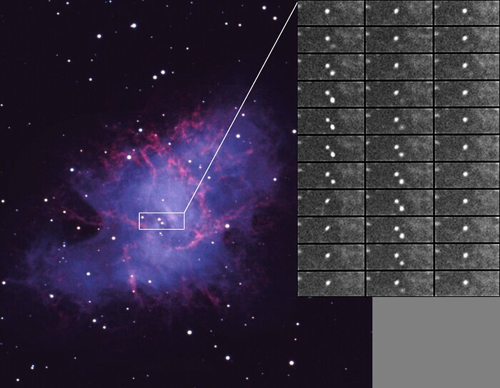
Fig. 12.14 A sequence of images showing the flashes at visible wavelengths from the Crab pulsar in the SNR. (Carroll & Ostlie (2007); Image Credit: N.A.Sharp/NOIRLab/NSF/AURA ).#

Fig. 12.15 A glitch in the Vela pulsar. (Carroll & Ostlie (2007); Figure adapted from McCulloch et al., Aust. J. Phys. 40, 725, 1987).#
12.7.2.2. Geminga#
One of th nearest pulsars is only ~90 pc away. Geminga (PSR 0633+1746) was a well known strong source of gamma rays for 17 years before it was identified as a pulsar in 1992. Geminga pulses with a period of 0.237 s in both gamma and X-rays (but not in the radio). It may display glitches and in visible light, its absolute magnitude is fainter than +23.
12.7.2.3. Evidence for a Core-Collapse Supernova Origin#
Only a few percent of pulsars are known to belong in binary systems. Pulsars also move much faster through space than do normal stars, sometimes with speeds \(\gtrsim 1000\ {\rm km/s}\). Both of these observations are consistent with a supernova origin for pulsars because a core-collapse supernova doesn’t have to be perfectly spherically symmetric. The forming pulsar could receive a kick that could eject it from a binary system. One hypothesis is that the pulsar is formed with an associated asymmetric jet, which could launch the pulsar (like a jet engine) at high speed away from its formation point.
12.7.3. Synchrotron and Curvature Radiation#
Observations of the Crab Nebula reveal its intimate connection with pulsar at its center, where the expanding nebula produces a ghostly glow surrounding gaseous filaments. If the present rate of expansion is extrapolated backward in time, the nebula converse to a point about 90 years after the supernova explosion was observed. The supernova must have been expanding more slowly in the past, which implies that the expansion is actually accelerating.
Iosif Shklovsky proposed in 1953 that the white light is synchrotron radiation produced when relativistic electrons spiral along magnetic field lines. Starting from the equation for magnetic force \(\mathbf{F}_m\) on a moving charge \(q\),
where the component of an electron’s velocity \(\mathbf{v}\) that is perpendicular to the field lines produces a circular motion around the lines and the velocity component that is parallel to the lines is not affected. The relativistic electrons accelerate and emit EM radiation as the follow the curved field lines. It is called synchrotron radiation if the circular motion dominates or curvature radiation, if the motion is primarily along the field lines.

Fig. 12.16 Synchrotron radiation emitted by a relativistic electron as it spirals around a magnetic field line. (Carroll & Ostlie (2007))#
In both cases, the energy distribution of the emitting electrons modulates the shape of the continuous spectrum, which easily distinguishes it from a spectrum of a normal blackbody. The radiation is strongly linearly polarized along the direction of the electron’s motion. Shklovsky predicted that the white light from the Crab Nebula would be strongly linearly polarized. His prediction was confirmed as the light from some emitting regions of the nebula was measured as 60% linearly polarized.
12.7.3.1. The Energy Source for the Crab’s Synchrotron Radiation#
The explanation of the white glow as synchrotron radiation raised questions because it implied that magnetic fields must permeate the Crab Nebula. According to theoretical estimates, this was a puzzle as the expansion of the nebula should have weakened the magnetic field far below \(\sim 10^{-7}\ {\rm T}\). The electrons should have radiated away all of their energy after 100 years. Continuous injection of new energetic electrons and a replenishment of the magnetic fields are necessary to produce the observed synchrotron radiation of today. The total power needed for these effects is calculated to be \(\sim 5 \times 10^{31}\ {\rm W}\), or \(>10^5\ L_\odot\).
The energy source is the rotating neutron star at the heart of the Crab Nebula that acts like a huge flywheel and stores an immense amount of rotational kinetic energy. As the star slows down, its energy supply decreases. To calculate the rate of energy loss, we write the rotational kinetic energy in terms of the period and moment of inertia of the neutron star as:
Then the rate of energy loss is
Exercise 12.6
What is the moment of inertia for the Crab pulsar assuming mass \(M = 1.4\ M_\odot\), and a radius \(R = 10\ {\rm km}\)? What is the energy loss?
Assuming that the neutron star is a uniform sphere, we have
Using the values of the rotation period and its derivative from Lyne et al. (2014), we have the pulsar period \(P = 0.033392412\ {\rm s}\) and the period’s rate of change \(\dot{P} = 4.2097160 \times 10^{-13}\). The energy loss is
This is exactly the energy needed to power the Crab Nebula. The slowing down of the neutron star flywheel has allowed the nebula to continue shining and expanding for nearly 1000 years.
The energy is not transported to the nebula by the pulse itself, where the radio luminosity of the Crab’s pulse is \(\sim 10^{24}\ {\rm W}\), or 200 million time smaller than the energy rate delivered to the nebula. The pulse process is a minor component of the total energy-loss mechanism.
import numpy as np

M_sun = 1.989e30 #Mass of the Sun in kg
M_ns = 1.4*M_sun #Mass of neutron star in kg
R_ns = 1e4 #Radius of neutron star in m
P_ns = 0.033392412 #period of the Crab pulsar in sec
Pdot_ns = 4.2097160e-13 #period change from Lyne et al. 2014

I_ns = 0.4*M_ns*R_ns**2
print("The moment of inertia for the neutron star is %1.1e kg m^2." % I_ns)

Kdot_ns = 4*np.pi**2*I_ns*Pdot_ns/P_ns**3
print("The energy loss of the pulsar is %1.1e W." % Kdot_ns)
The moment of inertia for the neutron star is 1.1e+38 kg m^2.
The energy loss of the pulsar is 5.0e+31 W.
12.7.3.2. The Structure of the Pulses#
The pulses are brief and are received over a small fraction of the pulse period (\(\sim\) 1-5%). Generally, they are received between 20 MHz and 10 GHz in the radio. AS the pulses travel through interstellar space, they are modified by electrons that they encounter along the way through their time-varying electric fields. This process slows the radio waves so that their speed is less than the speed of light in a vacuum and a greater retardation (i.e., slowing) occurs at lower frequencies. The sharp pulse emitted at the neutron star (with all the frequencies peaking at the same time) is gradually dispersed as it travels to Earth. More distant pulsars exhibit a greater pulse dispersion and these time delays can be used to measure the distances to pulsars. From these distance measurements, we find that pulsars are concentrated within the plane of our Milky Way Galaxy at distances of 100-1000s of parsecs.

Fig. 12.17 Pulses from PSR 0329+54 with a period of \(0.714\ {\rm s}\). (Carroll & Ostlie (2007); Figure adapted from the book Pulsars by Manchester & Taylor (1977))#
An integrated pulse profile is an average built up by adding together a train of 100 or more pulses, which shows to be remarkably stable. Some pulsars have more than one average pulse profile and abruptly switch back-and-forth between them. The subpulses may appear at random dimes in the “window” of the main pulse, or they may march across as drifting subpulses. For about 30% of all known pulsars, the individual pulses may simply disappear (or null), only to reappear up to 100 periods later. Drifting subpulses may even emerge from a nulling event in step with those that entered the null. The radio waves of many pulsars are strongly linearly polarized (up 100%), which indicates the presence of a strong magnetic field.

Fig. 12.18 Dispersion of the pulse from PSR 1641-45. (Carroll & Ostlie (2007); Figure from Pulsar Astronomy by Lyne & Graham-Smith (1990))#

Fig. 12.19 Sky map in Galactic coordinates showing (in green) the portions of the Galactic plane being targeted by the PALFA survey. This region corresponds to most of the Galactic plane visible with the Arecibo telescope. The dots correspond to known pulsars, their color indicates their inferred distance. Image Credit: Wikipedia:Palfa_Survey#

Fig. 12.20 The average of 500 pulses (top) and a series of 100 consecutive pulses (below) for PSR 1133+16. (Carroll & Ostlie (2007); Figure adapted from Cordes, Space Sci. Review, 24, 567, 1979)#

Fig. 12.21 Changes in the integrated pulse profile of PSR 1237+25 due to mode switching. This pulsar displays five distinct subpulses. (Carroll & Ostlie (2007); Figure adapted from Bartel et al., Ap. J., 258, 776, 1982)#

Fig. 12.22 Drifting subpulses for two pulsars; note that PSR 0031-07 also nulls. (Carroll & Ostlie (2007); Figure from Taylor et al., Ap. J., 195, 513, 1975)#
12.7.4. The Basic Pulsar Model#
The basic pulsar model consists of a rapidly rotating neutron star with a strong dipole magnetic field (i.e., north and south poles) that is incline to the rotation axis at an angle \(\theta\). To begin constructing the model, we need to obtain a measure of the pulsar’s magnetic field strength. As the pulsar rotates, the magnetic field at any point in space will change rapidly. According to Faraday’s law, this will induce an electric field at that point.

Fig. 12.23 A basic pulsar model. (Carroll & Ostlie (2007))#
Far from the star (near the light cylinder) the time-varying electric and magnetic fields form an EM wave tha carries energy away from the star, which is called the magnetic dipole radiation. The energy per second emitted by the rotating magnetic dipole is
which depends on the magnetic field strength \(B\) at the pole of the star, with a radius \(R\). The negative sign indicates that the neutron star is drained of energy, which causes its rotation period \(P\) to increase. The dependence on the pulsar period by \(1/P^4\) means that the neutron star will lose energy more quickly at shorter periods. The average pulsar period is 0.79 s and most pulsar are born spinning considerably faster than their current rates with typical initial periods of a few milliseconds.
Assuming that all of the rotational kinetic energy lost by the star is carried away by magnetic dipole radiation, we have
which can be solved for the magnetic field at the pole of the neutron star as
Exercise 12.7
What is an estimate of the magnetic field strength (at the poles) of the Crab pulsar?
For the Crab pulsar, we have measurements (Lyne et al. (2014)) of the period \(P = 0.033392412\ {\rm s}\) and its derivative \(\dot{P} = 4.209716 \times 10^{-13}\). Assuming that \(\theta = 90^\circ\) and from previous problems, we have that the radius of the pulsar \(R = 10\ {\rm km}\) and the moment of inertia \(I = 1.1 \times 10^{38}\ {\rm kg m^2}\). Then we can use these values to solve for \(B\) in
The pulsar is interacting with gas and dust in the surrounding nebula, which contributes to the slowing down the pulsar’s spin. The above value is an overestimate, where the accepted value is half as much (\(B = 4 \times 10^8\ {\rm T}\)).
Exercise 12.8
What is an estimate of the magnetic field strength (at the poles) of PSR 1937+214?
Kaspi, Taylor, & Ryba (1994) have measured the period \(P = 0.00155780646889794\ {\rm s}\) and its derivative \(\dot{P} = 1.051193 \times 10^{-19}\). Assuming a similar radius as the Crab pulsar (and moment of inertia), the magnetic field strength is
This much smaller value distinguishes the millisecond pulsars and provides another hint that these fastest pulsars may have a different origin or environment.
from scipy.constants import c, mu_0
import numpy as np

I_ns = 1.1e38 #moment of inertia of Crab pulsar in kg m^2
P_ns = 0.033392412 #pulse period in sec from Lyne et al. (2014)
dP_ns = 4.209716e-13 #derivative of the pulse period
R_ns = 1e4 #radius of the Crab pulsar

def B_ns(P,Pdot):
    #P = Period of the pulsar in sec
    #Pdot = time derivative of the pulse period
    return np.sqrt(3*mu_0*c**3*I_ns*P*Pdot)/((2.*np.pi)**1.5 * R_ns**3)

print("The magetic field strength of the Crab Pulsar is approximately %1.1e T."  % B_ns(P_ns,dP_ns))

P_ns = 0.00155780646889794 #pulse period in sec from Kaspi, Taylor, & Ryba (1994)
dP_ns = 1.051193e-19 #derivative of the pulse period

print("The magetic field strength of PSR 1937+214 is approximately %1.1e T."  % B_ns(P_ns,dP_ns))
The magetic field strength of the Crab Pulsar is approximately 8.0e+08 T.
The magetic field strength of PSR 1937+214 is approximately 8.6e+04 T.
12.7.4.1. Correlation Between Period Derivatives and Pulsar Classes#
The distribution of period derivatives for pulsars as a function of pulsar period shows that the vas majority of pulsars fall into a large grouping near \(\log_{10}\ P = -0.25\) or \(\sim 0.5\ {\rm s}\). The millisecond pulsars show a clear correlation with pulsars known to exist in binary systems. Other evident features are:
Pulsars known to emit energy at X-ray wavelengths have the longest periods and the largest period derivatives.
High-energy pulsars that emit energies from the radio to the IR (or higher frequencies) tend to have larger values of \(\dot{P}\), but otherwise typical periods.
Nearly all of the pulsars represented have \(\dot{P}>0\) (i.e., slowing down), where some of them have \(\dot{P} < 0\) (i.e., speeding up!).

Fig. 12.24 The time derivative of period \(\dot{P}\) as a function of the period \(P\). (Carroll & Ostlie (2007); Data from Manchester, Teoh, and Hobbs, A. J., 129, 1993, 2005, with an associated catalog )#
12.8. Homework#
Problem 1
Estimate the ideal gas pressure and the radiation pressure at the center of Sirius B, using \(3 \times 10^7\ {\rm K}\) for the central temperature. Compare these values with the estimated central pressure, Eq. (12.1).
Problem 2
The helium absorption lines seen in the spectra of DB white dwarfs are formed by excited \({\rm He\ I}\) atoms with one electron in the lowest (\(n = 1\)) orbital and the other in an \(n = 2\) orbital. White dwarfs of spectral type DB are not observed with temperatures below about 11,000 K.
Using what you know about spectral line formation, give a qualitative explanation why the helium lines would not be seen at lower temperatures. As a DB white dwarf cools below 12,000 K, into what spectral type does it change?
Problem 3
The most easily observed white dwarf in the sky is in the constellation of Eridanus (the River Eridanus). Three stars make up the 40 Eridani system: 40 Eri A is a 4th-magnitude star similar to the Sun; 40 Eri B is a 10th-magnitude white dwarf; and 40 Eri C is an 11th-magnitude red M5 star. This problem deals only with the latter two stars, which are separated from 40 Eri A by 400 AU.
(a) The period of the 40 Eri B and C system is 247.9 years. The system’s measured trigonometric parallax is \(0.201^{\prime\prime}\) and the true angular extent of the semimajor axis of the reduced mass is \(6.89^{\prime\prime}\). The ratio of the distances of 40 Eri B and C from the center of mass is \(a_B/a_C = 0.37\). Find the mass of 40 Eri B and C in terms of the mass of the Sun.
(b) The absolute bolometric magnitude of 40 Eri B is 9.6. Determine its luminosity in terms of the luminosity of the Sun.
(c) The effective temperature of 40 Eri B is 16,900 K. Calculate its radius, and compare your answer to the radii of the Sun, Earth, and Sirius B.
(d) Calculate the average density of 40 Eri B, and compare your result with the average density of Sirius B. Which is more dense, and why?
(e) Calculate the product of the mass and volume of both 40 Eri B and Sirius B. Is there a departure from the mass–volume relation? What might be the cause?
Problem 4
If our Moon were as dense as a neutron star, what would its diameter be?
Problem 5
Estimate the neutron degeneracy pressure at the center of a \(1.4\ M_\odot\) neutron star (take the central density to be \(1.5 \times 10^{18}\ {\rm kg/m^3}\)), and compare this with the estimated pressure at the center of Sirius B.