4. The Classification of Stellar Spectra

The science of astronomy progressed from a purely observational science of classification (prior to the 1800s) to a science interested in the fundamental inner workings of the stars (after the 1800s). As early as 1817, stars were known to be chemically different through their spectra.

4.1. The Formation of Spectral Lines

4.1.1. The Spectral Types of Stars

The initial spectral taxonomy used capital letters (from A…Z) that denoted the strength (or broadness) of the hydrogen absorption lines in a star and was developed by Edward Pickering and Williamina Fleming (Pickering’s assistant) in the 1890s at Harvard. Pickering had many assistants working with him at the time, where several of them developed different classification schemes. Antonia Maury’s scheme used the width of the spectral lines, which would have rearranged the Pickering’s B stars to come before the A stars. Building on Maury’s work, Annie Jump Cannon rearranged the sequence of spectra so that O stars came before B and A stars, added subdivisions (e.g., A0-A9), and consolidated many of the classes. As a result, the Harvard classification scheme became a temperature sequence with seven spectral types (OBAFGKM) with O stars being the hottest. Due to the reordering of letters, astronomy students developed mnemonics to remember the string of spectral types. The traditional mnemonic and some other memorable versions are:

• Oh Be A Fine Girl/uy, Kiss Me.

• Old, Bald, And Fat Generals Keep Mistresses.

• Oh Boy, An F Grade Kills Me.

• Only Boring, Astronomers Find Gratitude Knowing Mnemonics.

Can you do better?

Stars near the beginning of a given spectral type are referred to as early-type stars (e.g., A0), where those closer to the end are called late-type (e.g., A9). Cannon classified around 200,000 spectra, where the results were collected into the Henry Draper Catalogue. The catalog bears the name of Henry Draper because he was one of the first to photograph and classify a star based on its spectral lines (e.g., Vega), and Pickering supervised photographic spectroscopy at Harvard College Observatory after Draper’s death. Draper’s widow funded Pickering’s research under the Henry Draper Memorial. today many stars are referred to by their HD numbers (e.g., Betelguese is HD 39801).

Although we now know that Cannon’s classification scheme is based on surface temperatures, the physical basis of the Harvard spectral classification remained obscure to those who developed it. Vega (A0) displays very strong hydrogen absorption lines compared to the Sun (G2), but the Sun has stronger calcium absorption lines. This apparent dichotomy led to the following questions:

• Is this a result of a compositional difference between the stars?

or

• Are the different surface temperatures responsible for the relative strengths of the absorption lines?

The theoretical understanding of the quantum atom unlocked the secrets to stellar spectra. Absorption lines are created when an atom absorbs a photon with exactly the energy required for an electron to make an upward transition between energy levels. Emission lines are formed by the inverse process. The distinction between spectra of stars with different temperatures are due to the electrons occupying different atomic orbitals in the atmospheres of these stars. The details of spectral lines are complicated by the potential ionization stage of the the atoms. Note: an atom’s ionization stage is denoted by a Roman numeral (e.g., Ca II is singly ionized calcium).

Table 4.1 Harvard spectral classification.

Spectral Type	Color	Effective Temperature	Characteristics
O	Blue-white	\(\geq \text{30,000}\ {\rm K}\)	Strong \(\rm He\ II\) absorption/emission \(\rm He\ I\) absorption becoming stronger
B	Blue-white	\(\text{10,000-30,000}\ {\rm K}\)	\(\rm He\ I\) absorption strongest at B2 \(\rm H\ I\) absorption becoming stronger
A	White	\(\text{7500-10,000}\ {\rm K}\)	Balmer absorption lines strongest at A0 \(\rm Ca\ II\) absorption becoming stronger
F	Yellow-white	\(\text{6000-7500}\ {\rm K}\)	\(\rm Ca\ I\) lines strengthen as Balmer lines weaken Neutral metal absorption (\(\rm Fe\ I\), \(\rm Cr\ I\))
G	Yellow	\(\text{5200-6000}\ {\rm K}\)	Solar-type spectra \(\rm Ca\ II\), \(\rm Fe\ I\), and other neutral metals strengthen
K	Orange	\(\text{3700-5200}\ {\rm K}\)	Strong \(\rm Ca\ II\ H\ \&\ K\) lines Spectra dominated by metals
M	Red	\(\text{2400-3700}\ {\rm K}\)	Spectra dominated by molecular absorption (oxides) Neutral metals remain strong
L	Dark red	\(\text{1300-2400}\ {\rm K}\)	Stronger in IR than in visible Strong molecular absorption in metal hydrides (\(\rm FeH\)), water, carbon monoxide, and alkali metals Molecular absorption in oxides weakening
T	Infrared	\(\leq \text{1300}\ {\rm K}\)	Strong methane (\(\rm CH_4\)) bands Weakening carbon monoxide (\(\rm CO\)) bands

In Cannon’s classification scheme, the Balmer lines (hydrogen absorption) reach their maximum intensity when the effective surface temperature of the star reaches 10,000 K. The visible neutral Helium (He I) lines occur at 22,000 K (B2 stars) and singly ionized calcium (Ca II) are most intense at 5250 K (K0 stars). In astronomy, spectral lines of Ca II H and K are quoted, which are 396.8 nm and 393.3 nm, respectively. Also, astronomers use the term metal to refer to a chemical element heavier than helium because hydrogen and helium are the most abundant elements in the universe. Table 4.1 includes the traditional Harvard classification scheme and the spectral types of very cool stars (L-Type) and brown dwarfs (T-Type). Brown dwarfs are objects with too lite mass for nuclear fusion (of hydrogen) to occur in their interiors and are not considered stars. Figure 4.1 illustrates how the spectra appear for a range of spectral classes (falsely colored). Figure 4.2 demonstrates the resultant spectra after analysis and digitization.

Fig. 4.1 Montage of false color spectra for main-sequence stars. Image credit: Wikipedia

Fig. 4.2 A stack of all of the spectral images showing how the spectral features change systematically from types O5 through M5. Image credit: Jacoby, Hunter, & Christian (1984); adapted by Richard Pogge

4.1.2. The Maxwell-Boltzmann Velocity Distribution

Electronic transitions explained the existence of absorption or emission spectral lines, but there must be some underlying physical foundation for the relative strength of spectral lines. If the probability of transition was equal (independent of the orbital), then the absorption line strength of the Balmer lines should be equal. This is clearly not the case as demonstrated by Figs. 1 and 2. Then, two basic questions arise:

1. In what orbitals are electrons most likely to be found?

2. What are the relative numbers of atoms in various stages of ionization?

Answering the first question will provide insight into which spectral lines we expect to be stronger than the other spectral lines. While the second question will probe the relative strengths of the spectral lines. The answers to both question are found in statistical mechanics, which is a branch of physics that studies the statistical properties of many body systems. For example, a gas contains a huge number of particles and it would be impossible to calculate the detailed behavior of all the particles. Information about how the behavior of the system can be determined using well-defined properties, such as its internal energy (temperature), pressure, and density.

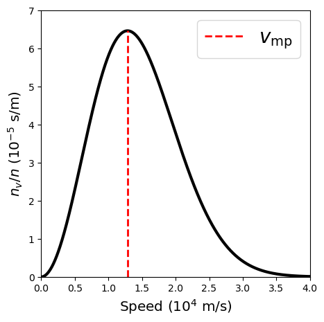
For a gas in thermal equilibrium (i.e., the gas in not rapidly changing in temperature), the Maxwell-Boltzmann velocity distribution function describes the number density of gas particles \(n\) within a given range of speed \(v\). The number of gas particles per unit volume having speeds between \(v\) and \(v+dv\) is given by

(4.1)\[n_v dv = n \left(\frac{m}{2\pi kT}\right)^{3/2} e^{-mv^2/(2kT)}4\pi v^2 dv,\]

which depends on the total number density \(n\), the particle’s mass \(m\), the Boltzmann constant \(k\), and the temperature of the gas \(T\) (in K).

The exponent of the Maxwell-Boltzmann distribution function is the ratio of a gas particle’s kinetic energy (\(\frac{1}{2}mv^2\)) to the characteristic thermal energy (\(kT\)). Particles above the thermal energy tend to either can escape so the overall distribution remains the same. This is analogous as to why the temperature of a pot of boiling water doesn’t keep increasing. The distribution peaks when the particle energies are equal at a most probable speed of

(4.2)\[\begin{align} v_{\rm mp} = \sqrt{\frac{2kT}{m}}. \end{align}\]

Exercise 4.1

What is the most probable speed for hydrogen atoms in an A0 spectral-type star?

The most probable speed depends on the temperature \(T\) of a gas and the mass \(m\) of the average particle. For an A0 spectral-type star, the effective surface temperature \(T_{e}\) is \(10^4\ {\rm K}\), while the outer atmosphere is mostly hydrogen, or \(m = m_{\rm H} = 1.67\times 10^{-27}\ {\rm kg}\). Using these factors, we calculate the most probable speed \(v_{\rm mp}\) as,

\[\begin{align*} v_{\rm mp} &= \sqrt{\frac{2kT_e}{m_{\rm H}}}, \\ &= \sqrt{\frac{2(1.38\times 10^{-23})(10^4)}{1.67 \times 10^{-27}}} = 1.29 \times 10^4\;{\rm m/s}. \end{align*}\]

import numpy as np
import matplotlib.pyplot as plt 
from scipy.constants import k, m_p

def Maxwell_Boltzmann(v,dv):
    #v = velocity
    #dv = velocity interval
    factor = m_H/(2*k*T_eq)
    MB = (factor/np.pi)**1.5*np.exp(-factor*v**2)*(4*np.pi*v**2)
    return MB

T_eq = 10000 #K; surface temperature of an A0 star
#k = 1.380649e-23 #J/K; Boltzmann constant
m_H = m_p #1.67e-27 #kg; mass of hydrogen 

v_rng = np.arange(0,4e4,2) #velocity range in m/s
nv_n = np.zeros(len(v_rng))
for i in range(0,len(v_rng)-1):
    nv_n[i] = Maxwell_Boltzmann(v_rng[i],2)

v_mp = v_rng[np.argmax(nv_n)]
fs = 'x-large'
fig = plt.figure(figsize=(5,5),dpi=100)
ax = fig.add_subplot(111)

ax.plot(v_rng/1e4,nv_n/1e-5,'k-',lw=3)
ax.axvline(v_mp/1e4,0,np.max(nv_n)/7e-5,linestyle='--',color='r',lw=2,label='$v_{\\rm mp}$')

ax.legend(loc='best',fontsize=20)
ax.set_ylim(0,7)
ax.set_xlim(0,4)

ax.set_ylabel("$n_v/n$ ($10^{-5}$ s/m)",fontsize=fs)
ax.set_xlabel("Speed ($10^4$ m/s)",fontsize=fs)


print("The most probable speed for hydrogen atoms in an A0 star is %1.2e m/s." % v_mp)

The most probable speed for hydrogen atoms in an A0 star is 1.28e+04 m/s.

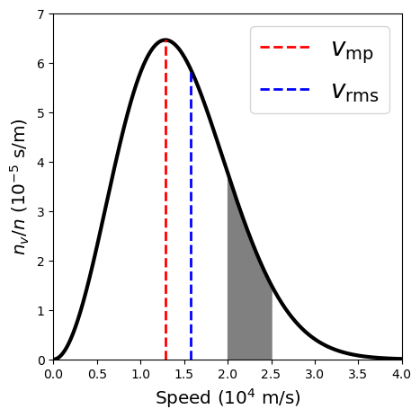
The high-speed exponential “tail” of the distribution function results in a somewhat higher root-mean-square speed of

(4.3)\[\begin{align} v_{\rm rms} = \sqrt{\frac{3kT}{m}}. \end{align}\]

The area under the curve of the Maxwell-Boltzmann distribution is the fraction of gas particles within a range of speeds or,

(4.4)\[\begin{split}N/N_{\rm total} &= \frac{1}{n}\int_{v_1}^{v_2} n_v dv, \\ &= \left(\frac{m}{2\pi kT}\right)^{3/2} \int_{v_1}^{v_2} e^{-mv^2/(2kT)} 4\pi v^2 dv.\end{split}\]

Equation (4.4) has a closed-form solution when \(v_1 = 0\) and \(v_2\rightarrow \infty\), it must be evaluated numerically in other cases.

Exercise 4.2

What is the root-mean-square speed of the hydrogen atoms in an A0 star?

The root-mean-square (\(v_{\rm rms}\)) speed of gas particle is similar to the most probable speed, where they are related by a factor of \(\sqrt{3/2}\). Therefore, we calculate \(v_{\rm rms}\) using this factor to get,

\[\begin{align*} v_{\rm rms} &= \sqrt{\frac{3kT}{m}} = \sqrt{\frac{3}{2}}v_{\rm rms}, \\ & = 1.57 \times 10^4\ {\rm m/s}. \end{align*}\]

Exercise 4.3

What is the fraction of gas particles with speeds between 20-25 km/s?

The fraction of gas particles between a speed \(v_1\) and \(v_2\) is determined by integrating the Maxwell-Boltzmann distribution (Eq. (4.4)). The indefinite integral of Eq. (4.4) introduces the error function \(\rm erf(z)\) (see the result in Wolfram Alpha). Therefore, we employ Simpson’s rule to evaluate the integral. The result of this numerical method (see the python code below) is

\[\begin{align*} N/N_{\rm total} = 0.128,\ \text{or } 12.8\%. \end{align*}\]

import numpy as np

v_rms = np.sqrt((3*k*T_eq)/m_H) #using Eqn 3
vrms_idx = np.where(np.abs(v_rms-v_rng)<1)[0]
vrng_idx = np.where(np.logical_and(v_rng>=2e4,v_rng<=2.5e4))[0]

def Simpsons_rule(a,b,N,func):
    #width of each interval
    h = (b-a)/float(N-1)
    tot_sum = 0

    for i in range(1,N):
        x_left = a + (i-1)*h
        x_right = a + i*h
        x_mid = x_left + h/2
        tot_sum += (h/6.)*(func(x_left,h)+4*func(x_mid,h)+func(x_right,h))
    return tot_sum

frac_rng = Simpsons_rule(2e4,2.5e4,10,Maxwell_Boltzmann)

fs = 'x-large'
fig = plt.figure(figsize=(5,5),dpi=100)
ax = fig.add_subplot(111)

ax.plot(v_rng/1e4,nv_n/1e-5,'k-',lw=3)
ax.axvline(v_mp/1e4,0,np.max(nv_n)/7e-5,linestyle='--',color='r',lw=2,label='$v_{\\rm mp}$')
ax.axvline(v_rms/1e4,0,float(nv_n[vrms_idx])/7e-5,linestyle='--',color='b',lw=2,label='$v_{\\rm rms}$')

ax.fill_between(v_rng[vrng_idx]/1e4,0,nv_n[vrng_idx]/1e-5,color='gray')

ax.legend(loc='best',fontsize=20)

ax.set_ylim(0,7)
ax.set_xlim(0,4)

ax.set_ylabel("$n_v/n$ ($10^{-5}$ s/m)",fontsize=fs)
ax.set_xlabel("Speed ($10^4$ m/s)",fontsize=fs)

print("The v_rms for the hydrogen atoms is %1.2e m/s." % v_rms)
print("The fraction of gas particles between 20-25 km/s is %1.3f or %2.1f%%." % (frac_rng,frac_rng*100))

The v_rms for the hydrogen atoms is 1.57e+04 m/s.
The fraction of gas particles between 20-25 km/s is 0.128 or 12.8%.

The Maxwell-Boltzmann distribution function describes the kinetic energy of gas particles within a star’s atmosphere at an effective temperature \(T_e\) and allows us to derive the most probable speed \(v_{mp}\) of the particles. Recall our first question was to determine the most likely orbitals for the electrons. While this cannot be answered fully yet, the next step will estimate the relative likelihood of a possible energy level through the Boltzmann equation.

4.1.3. The Boltzmann Equation

Collisions between gas particles cause some particles to gain and lose energy and thus, produce a definite distribution in the speeds of gas particles. Statistical mechanics shows that orbitals of higher energy are less likely to be occupied by electrons. Suppose there are two states of Energy \(E_a\) and \(E_b\) that are represented by a set of quantum numbers \(s_a\) and \(s_b\), respectively.

Note

If the first state \(E_a\) is the ground state of hydrogen (\(E_a = -13.6\) eV), then its quantum state is \(s_a = \{1,0,0,+1/2\}\); in general, the individual elements are the quantum numbers, \(\{n,\ell,m_\ell,m_s\}\). See Table 4.2 for a listing of the quantum numbers of for the ground (\(n=1\)) and 1st excited (\(n=2\)) states.

Table 4.2 Quantum Numbers for the Hydrogen Atom.

\(n\)	\(\ell\)	\(m_\ell\)	\(m_s\)
1	0	0	+1/2
1	0	0	-1/2
2	0	0	+1/2
2	0	0	-1/2
2	1	1	+1/2
2	1	1	-1/2
2	1	0	+1/2
2	1	0	-1/2
2	1	-1	+1/2
2	1	-1	-1/2

There exists some probability \(P(s_x)\) that the system is in a state \(s_x\). Then the ratio of the probability between orbital states represents the likelihood for which electrons may be found. Using the states \(s_a\) and \(s_b\), the ratio of probability is given by

(4.5)\[\begin{align} \frac{P(s_b)}{P(s_a)} = \frac{e^{-E_b/(kT)}}{e^{-E_a/(kT)}} = e^{-(E_b-E_a)/(kT)}, \end{align}\]

Note

An alternate form of the Boltzmann constant is \(8.617333262145 \times 10^{-5}\) eV/K, which is useful for solving problems when the energy is given in eV.

where \(T\) is the common temperature of the two systems and \(e^{-E_x/(kT)}\) represents the Boltzmann factor for a state \(s_x\). Suppose that \(E_b > E_a\) and the temperature is decreasing (\(T\rightarrow 0\)), then the factor in the exponential \(-(E_b-E_a)/(kT) \rightarrow -\infty\) and so the ratio of probability \(P(s_b)/P(s_a) \rightarrow 0\). This means that there isn’t any thermal energy available to excite the electron to a higher energy level. Conversely, if there is an infinite amount of energy (i.e., \(T\rightarrow \infty\)), then it is certain that an excitation will occur because \(P(s_b)/P(s_a) \rightarrow 1\).

It is often the case that then energy levels of the system may be degenerate, where more than one quantum state can have the same energy. For example, two electrons in the ground state of hydrogen with opposite spins will have the same energy because \(E_n\) doesn’t depend on the quantum number \(m_s\). Table 4.2 shows two states for the ground (\(n=1\)) state and eight states for the 1st excited (\(n=2\)) state so that the number of degenerate states \(g_n = 2n^2\). When taking averages, we must account for the degenerate states using a separate factor \(g_x\), which is the statistical weight of the energy level. The ratio of the probability between two degenerate states is given by

(4.6)\[\frac{P(s_b)}{P(s_a)} = \frac{g_b e^{-E_b/(kT)}}{g_a e^{-E_a/(kT)}} = \frac{g_b}{g_a} e^{-(E_b-E_a)/(kT)} = \frac{N_b}{N_a},\]

which is typically indistinguishable from the ratio of the number of atoms \(N_b/N_a\) because stellar atmospheres contain a vast number of atoms. Equation (4.6) is also called the Boltzmann equation.

Exercise 4.4

At what temperature will equal numbers of atoms have electrons in the ground and 1st excited states?

The ratio of the number of atoms between the 1st excited and ground states is \(N_2/N_1\). If these are in equal amounts, then the ratio is equal to unity. To account for the degeneracy between states, we recall that \(g_2 = 8\) and \(g_1 = 2\). Finally, we can use the Boltzmann equation, along with the energy equation for hydrogen \(E_n = 13.6/n^2\) eV to get,

\[\begin{align*} 1= \frac{8}{2}e^{-[(-13.6/4 \;{\rm eV})-(-13.6 \;{\rm eV})]/(kT)}. \end{align*}\]

Solving for the exponential, we get

\[\begin{align*} 4^{-1} = e^{-10.2\;{\rm eV}/(kT)} \end{align*}\]

and taking the logarithm of both sides to get

\[\begin{align*} \frac{10.2\;{\rm eV}}{kT} = \ln(4). \end{align*}\]

Solving for the temperature yields,

\[\begin{align*} T = \frac{10.2\;{\rm eV}}{8.6173333\times 10^{-5}\;{\rm eV/K}\cdot\ln(4)} = 85,400\;{\rm K}. \end{align*}\]

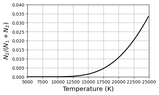
Extremely high temperatures are required for a significant number of hydrogen atoms to have electrons in the 1st excited state, where we have shown what it takes to get equal amounts. Exploring all the possible ratios \(N_2/N_{\rm tot}\) (or \(1/(1+N_1/N_2)\)) as a function of temperature \(T\) reveals that only a small fraction (\(\leq3.5\)%) of electrons will be in the 1st excited state even if the temperature reaches 25,000 K. We observe Balmer lines within stars at a much lower temperature (9520 K). There must be another piece to this puzzle and it is found in the Saha equation.

def Boltzmann_Eq_H12(T):
    #return the fraction of particles in the 1st excited 
    #state relative to the ground state of hydrogen (N_2/N_1)
    return 4*np.exp(-10.2/(k_boltz*T))

k_boltz = 8.6173333e-5 #eV/K
fs = 'x-large'

fig = plt.figure(figsize=(5,3),dpi=100)
ax = fig.add_subplot(111)

T_rng = np.arange(5000,2.5e4,100)
N2_Ntot = 1./(1+1/Boltzmann_Eq_H12(T_rng))
ax.plot(T_rng,N2_Ntot,'k-',lw=2)
ax.grid(True)

ax.set_xlabel("Temperature (K)",fontsize=fs)
ax.set_ylabel("$N_2/(N_1+N_2)$", fontsize=fs)

ax.set_xlim(5000,2.5e4)
#ax.set_yscale('log')
ax.set_ylim(0.0,0.04);

4.1.4. The Saha Equation

The Maxwell-Boltzmann equation does not provide a complete picture, which lies in also considering the relative number of atoms in different stages of ionization. Ionization energy is the requisite energy to remove an electron from an atom and thus, increasing its ionization stage by one (i.e., stage i to stage i+1). The ionization energy of hydrogen is 13.6 eV or the energy needed to convert it from H I to H II. However, not all electron transitions start from the ground state. An average must be taken over the orbital energies to allow for the possible partitioning of the atom’s electrons among its orbitals. The average is obtained using the partition function Z, which is the weighted sum of the number of ways the atom can arrange its electrons with the same energy. More energetic configurations receive less weight from the Boltzmann factor when the sum is taken. Let \(E_j\) be the energy of the jth energy level and \(g_j\) is the degeneracy of that level, then the partition function \(Z\) is

(4.7)\[Z = \sum_{j=1}^\infty g_j e^{-(E_j-E_1)/(kT)},\]

and is measured relative to the ground state energy \(E_1\). If we use the partition functions of two ionization stages (\(Z_i\) and \(Z_{i+1}\)), then the ratio of atoms in each stage is

(4.8)\[\frac{N_{i+1}}{N_i} = \frac{2Z_{i+1}}{n_eZ_i}\left(\frac{2\pi m_e kT}{h^2} \right)^{3/2} e^{-\chi_i/(kT)}, \]

where \(m_e\) is the mass of the electron, \(n_e\) is the number of free electrons per unit volume, and \(\chi_i\) is the ionization energy. The factor of 2 in front of the partition function \(Z_{i+1}\) reflects the two possible spins of the free electron, \(m_s = \pm 1/2\). Sometimes the pressure of the free electrons \(P_e\) is used in place of the electron number density using the ideal gas law (\(P_e = n_e kT\)). The electron pressure ranges from \(0.1-100 \;{\rm N/m^2}\) in the atmospheres of cooler and hotter stars, respectively.

Note

Equation (4.8) is known as the Saha equation, after the Indian astrophysicist Meghnad Saha.

4.1.5. Combining The Boltzmann and Saha Equations

The Boltzmann equation describes what is possible, where the Saha equation describes what is probable. Therefore, what we observe should be a combination of effects from both equations. Consider the degree of ionization in a stellar atmosphere consisting of pure hydrogen and that the electron pressure is a constant \(P_e = 20\;{\rm N/m^2}\). Hydrogen has only two states: neutral hydrogen (H I) and ionized hydrogen (H II). The fraction of atoms that are ionized depends on the ratio of the number ionized atoms \(N_{\rm II}\) and the total number of atoms \(N_{\rm tot}=N_{\rm I} + N_{\rm II}\). Ionized hydrogen is just a proton and thus, has no degeneracy and the partition function \(Z_{\rm II} = 1\). The partition function for the remaining neutral hydrogen (H I) is simply \(Z_{\rm I} \approx g_1 = 2(1)^2 = 2\). The temperatures of stellar atmospheres range from 5000 K - 25,000 K and the previous example (using the Boltzmann equation) showed that most electrons for the hydrogen atoms are in the ground state (\(n=1\)). For neutral hydrogen, equation 7 becomes

(4.9)\[\begin{align} Z_{\rm I} = g_1 e^{-(E_1-E_1)/(kT)} + g_2 e^{-(E_2-E_1)/(kT)} = g_1 + g_2 e^{-(E_2-E_1)/(kT)} , \end{align}\]

where the second term \(g_2 e^{-(E_2-E_1)/(kT)} \rightarrow 0\) because \(kT = 0.4-2.2\) eV for the appropriate temperature range and \(e^{-(E_2-E_1)/(kT)} \ll 1\). The ratio \(N_{\rm II}/N_{\rm tot}\) can be rewritten as

(4.10)\[\begin{align} \frac{N_{\rm II}}{N_{\rm tot}} = \frac{N_{\rm II}/N_{\rm I}}{1 + N_{\rm II}/N_{\rm I}}. \end{align}\]

Then the Saha equation can be used to determine the ratio \(N_{\rm II}/N_{\rm I}\). Using the ionization energy \(\chi_{\rm I} = 13.6\) eV for hydrogen, the ideal gas law, and substituting the values for \(Z_{\rm I}\) and \(Z_{\rm II}\) into Equation (4.6), the ratio \(N_{\rm II}/N_{\rm I}\) is given as

(4.11)\[N_{\rm II}/N_{\rm I} = \frac{kT}{P_e}\left(\frac{2\pi m_e kT}{h^2} \right)^{3/2} e^{-13.6\;{\rm eV}/(kT)}.\]

In the end, we want to know the fraction of ionized hydrogen atoms \(N_2/N_{\rm tot}\) present for a given temperature. The Boltzmann equation (Eqn. (4.6)) provides the fraction of atoms in a higher energy state and the Saha equation (Eqn. (4.11)) can be used to determine the fraction of atoms that are not ionized.

Note

If the atoms are ionized, then they can’t have the electron in a higher energy level.

Assuming that nearly all the atoms are in either the ground state or the first excited state, we can employ the approximation for ratio in the number of non-ionized (neutral) particles to the total number of particles, \(N_{\rm I}/(N_1 + N_2) \approx 1\), and write

(4.12)\[\frac{N_2}{N_{\rm total}} = \frac{N_2}{N_1+N_2} \frac{N_{\rm I}}{N_{\rm I}+N_{\rm II}} = \frac{N_2/N_1}{1 + N_2/N_1} \frac{1}{1+N_{\rm II}/N_{\rm I}}\]

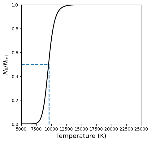
• Plot the fraction of ionized hydrogen as a function of temperature.

• Plot the fraction of hydrogen in the first excited state as a function of temperature.

def Saha_Eq_H12(P_e,T):
    #return the fraction of ionized particles (N_II/N_I) for a pure hydrogen gas
    kT = k_boltz*T
    Z_I = 2. + 8.*np.exp(-10.2/kT)
    return (2*kT/P_e)*(Z_II/Z_I)*(2.*np.pi*m_e*kT/h**2)**1.5*np.exp(-chi_I/kT)

k_boltz = 1.38064852e-23 #J/K
P_e = 20
#Convert to Joules because P_e is in N/m^2
chi_I = 13.6*1.60218e-19 #convert eV to J
m_e = 9.10938356e-31 #kg; mass of electron; https://en.wikipedia.org/wiki/Electron
h = 6.62607004e-34 #J/s Planck constant
Z_II = 1. 
fs = 'x-large'

fig = plt.figure(figsize=(5,5),dpi=100)
ax = fig.add_subplot(111)
T_rng = np.arange(5000,2.5e4,100)
NII_NI = Saha_Eq_H12(P_e,T_rng)
NII_Ntot = NII_NI/(1.+NII_NI)
ax.plot(T_rng,NII_Ntot,'k-',lw=2)

fifty_pct = np.where(np.abs(NII_Ntot-0.5)<0.025)[0]
if len(fifty_pct)>0:
    ax.axhline(0.5,0,float(T_rng[fifty_pct]-5000)/2e4,linestyle='--',lw=2)
    ax.axvline(T_rng[fifty_pct],0,0.5,linestyle='--',lw=2)
    print("Fifty percent ionization occurs at T ~ %4d K." % T_rng[fifty_pct])

ax.set_xlim(5000,25000)
ax.set_ylim(0,1)


ax.set_xlabel("Temperature (K)",fontsize=fs)
ax.set_ylabel("$N_{\\rm II}/N_{\\rm tot}$",fontsize=fs);

Fifty percent ionization occurs at T ~ 9600 K.

def Boltzmann_Eq_H12(T):
    #return the fraction of particles in the 1st excited 
    #state relative to the ground state of hydrogen (N_2/N_1)
    k_boltz = 8.6173333e-5 #eV/K
    return 4*np.exp(-10.2/(k_boltz*T))

N2_N1 = Boltzmann_Eq_H12(T_rng)
N2_Ntotal = N2_N1/(1.+N2_N1)*(1./(1.+NII_NI))/1e-6
T_max = np.argmax(N2_Ntotal)

fig = plt.figure(figsize=(5,5),dpi=100)
ax = fig.add_subplot(111)

ax.plot(T_rng,N2_Ntotal,'k-',lw=2)
ax.axvline(T_rng[T_max],0,np.max(N2_Ntotal)/9.,linestyle='--',lw=2)
print("The peak occurs at T ~ %4d K." % T_rng[T_max])

ax.set_xlim(5000,25000)
ax.set_ylim(0,9)

ax.set_xlabel("Temperature (K)",fontsize=fs)
ax.set_ylabel("$N_2/N_{\\rm total}$ ($10^{-6}$)",fontsize=fs);

The peak occurs at T ~ 9900 K.

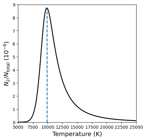
The peak at 9900 K is in good agreement with the observations. The diminishing strength of the Balmer lines at higher temperatures is due to the rapid ionization of hydrogen above 10,000 K. The narrow region inside of a star with a temperature \({\sim}\)10,000 K is called a hydrogen partial ionziation zone.

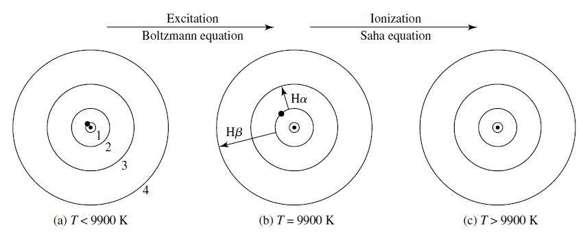
Fig. 4.3 The electron’s position in the hydrogen atom at different temperatures. (a) The electron is in the ground state. (b) The is excited from \(n=2\) to a higher energy level (i.e., Balmer lines). (c) The atom is ionized. Image credit: Carroll & Ostlie (2007)

Stellar atmospheres contain other elements (although predominantly composed of hydrogen) and the peak can range from about 7500 - 10,500 K depending on the electron pressure. There is typically 1 helium atom for every 10 hydrogen atoms and the presence of helium (with its extra electrons) provides more opportunities for hydrogen to recombine. A higher temperature is needed to obtain the same level of ionization once helium is added. The Saha equation can be applied only to a gas in thermodynamic equilibrium, where the Maxwell-Boltzmann velocity distribution is an accurate representation of the system. The gas density must be low (~1 \({\rm kg/m^3}\)) or the presence of neighboring ions will distort an atom’s orbitals and lower its ionization energy.

4.1.6. Application to the Sun

The Sun’s surface is a thin layer of its atmosphere called the photosphere, which a characteristic temperature \(T_e = 5777\) K, an electron pressure of about \(1.5\;{\rm N/m^2}\), and about 500,000 hydrogen atoms for each calcium atom. The Boltzmann and Saha equations provide the relative strengths of absorption due to the Balmer lines and the calcium (Ca II H and K) lines. Starting with the Balmer lines, we can use the Saha equation (Eqn. (4.11)) to determine the ratio of ionized to neutral hydrogen.

print("The ratio of ionized to neutral hydrogen is: %1.2e" % Saha_Eq_H12(1.5,5777))

The ratio of ionized to neutral hydrogen is: 7.70e-05

Thus, there is only one ionized hydrogen (H II) for every ~13,000 neutral hydrogen (H I) atoms. The Boltzmann equation (Eqn. (4.6)) reveals how many hydrogen atoms (with electrons) are in the first excited state.

print("The number of ratio of hydrogen atoms in the first excited state relative to the ground state is %1.2e" % Boltzmann_Eq_H12(5777))

The number of ratio of hydrogen atoms in the first excited state relative to the ground state is 5.05e-09

Combining the Boltzmann and Saha equations (Eqn. (4.12)) we get that the result is that only one of every ~200 million hydrogen atoms is in the first excited state and capable of producing Balmer lines.

NII_NI = Saha_Eq_H12(1.5,5777)
N2_N1 = Boltzmann_Eq_H12(5777)
N2_Ntotal = N2_N1/(1.+N2_N1)*(1./(1.+NII_NI))

print(N2_Ntotal)

5.05454248777915e-09

Turning to the calcium atoms, we need to modify our functions to the ionization energy of Ca I (\(\chi_I = 6.11\) eV) and use tabulated values for the partition functions \(Z_1 = 1.32\) and \(Z_2 = 2.30\) (Aller (1963)).

Note

The Saha equation is sensitive to the ionization energy because \(\chi/(kT)\) appears as an exponent and \(kT \approx 0.5\;{\rm eV} \ll \chi\). Thus a small difference in the ionization energy produces a change of many powers of \(e\) in the Saha equation.

def Saha_Eq_Ca12(P_e,T,Z_I,Z_II):
    #return the fraction of ionized particles (N_II/N_I) for a pure hydrogen gas
    k_boltz = 1.38064852e-23 #J/K
    kT = k_boltz*T
    return (2*kT/P_e)*(Z_II/Z_I)*(2.*np.pi*m_e*kT/h**2)**1.5*np.exp(-chi_I/kT)

chi_I = 6.11*1.60218e-19 #J; ionization energy of Ca I
print("The ratio of ionized to neutral calcium is: %3d" % Saha_Eq_Ca12(1.5,5777,1.32,2.30))

The ratio of ionized to neutral calcium is: 918

Practically all of the calcium atoms are ionized, where there are ~900 Ca II atoms to every one Ca I. We can now use the Boltzmann equation to estimate the fraction of non-ionized calcium atoms that are also in the ground state. The first excited state of Ca II is \(E_2 - E_1 = 3.12\) eV above the ground state, where the degeneracies for these states are \(g_1 = 2\) and \(g_2 = 4\).

def Boltzmann_Eq_Ca12(T):
    #return the fraction of particles in the 1st excited 
    #state relative to the ground state of hydrogen (N_2/N_1)
    k_boltz = 8.6173333e-5 #eV/K
    E2_E1 = 3.12 #eV
    g_1, g_2 = 2., 4.
    return (g_2/g_1)*np.exp(-E2_E1/(k_boltz*T))

print("The number of ratio of calcium atoms in the first excited state relative to the ground state is %1.2e" % Boltzmann_Eq_Ca12(5777))

The number of ratio of calcium atoms in the first excited state relative to the ground state is 3.79e-03

Out of every ~265 Ca II ions, all but one are in the ground state and thus, capable of producing the CA II K line. This implies that nearly all of the calcium atoms are singly ionized (Ca II) and in the ground state.

\[ \left[\frac{N_1}{N_{\rm total}}\right]_{\rm Ca\;II} \approx \left[\frac{N_1}{N_1+N_2}\right]_{\rm Ca\;II} \left[\frac{N_{\rm II}}{N_{\rm total}}\right]_{\rm Ca} = \left(\frac{1}{1+0.00379}\right) \left(\frac{918}{1+918}\right) = 0.995 \]

N1_Ntot = (1./(1+0.00379))*(918./919.)
print(np.round(N1_Ntot,3))

0.995

The difference in strength between the Ca II H and K lines with the Balmer lines is due to relative abundance of atoms that are capable of producing the electron transitions. There are ~500,000 hydrogen atoms for every calcium atom, but only a small fraction of those hydrogen atoms are capable of producing Balmer lines (i.e., un-ionized and in the first excited state). By multiplying the number of hydrogen atoms relative to calcium by the fraction capable of producing the Balmer lines (from the Boltzmann Eq), we get

\[ \frac{500,000\;{\rm H}}{1\;{\rm Ca}} \times (5.06 \times 10^{-9}) \approx 0.00253\;\frac{{\rm H}}{\rm Ca} = \frac{1\;{\rm H}}{395\;{\rm Ca}}, \]

which shows that there are ~400 times more Ca II ions (with electrons in the ground state) than neutral hydrogen atoms (with electrons in the 1st excited state). The strength of the H and K lines is not due to a greater abundance of calcium in the Sun, rather the strength reflects the sensitivity for the excitation and ionization of atomic states. Figure 4.4 shows how the spectral line strength varies with stellar spectral type.

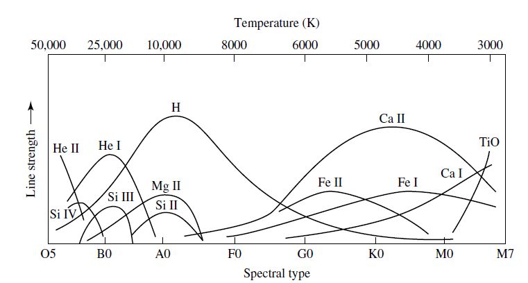
Fig. 4.4 The dependance of spectral line strengths on stellar spectral type (or surface temperature). Image credit: Carroll & Ostlie (2007)

In the early 20th century, it was the scientific consensus that if the Earth’s crust should be raised to the temperature of the Sun’s atmosphere, then it would give a very similar absorption spectrum. The observations of the time had only uncovered that many of the same elements of Earth’s crust were also in the Sun. Cecilia Payne-Gaposchkin showed in her 1925 PhD thesis the connection between the spectral types and ionization states. It was unclear at the time whether her interpretation would prove correct. But after a few years, others confirmed her results and then the importance of her work was realized.

4.2. The Hertzsprung-Russell Diagram

Early in the 20th century, the bigger picture of how to categorize began to come into focus, where the O stars tended to be brighter and hotter than the M stars. The study of binary stars uncovered an empirical mass-luminosity relationship, which showed that O stars are more massive than M stars. Astronomers proposed a theory of stellar evolution supposing that stars begin their lives as bright O stars and cool off/lose mass over time to become the fainter M stars. This idea remains in the terms early and late when discussing the range of stars between spectral types, but has otherwise been superseded by modern theories.

Note

Stellar evolution describes the change in the structure and composition of an individual star as it ages. This usage of the term differs from that in biology, which describes the changes that occur over generations.

4.2.1. An Enormous Range in Stellar Radii

One prediction of the idea of stellar cooling is there should be a relation between a star’s absolute magnitude and its spectral type. Ejnar Hertzsprung searched catalogs of stars and tabulated stars whose absolute magnitude and spectral types had been accurately determined. He confirmed the expected correlation between stellar luminosity and spectral type, but he also uncovered an anomaly within types G or later. These stars showed a range of magnitudes within the same spectral classification. Using the Stefan-Boltzmann law (\(L\propto R^2 T_e^4\)), the radii of stars (compared to the Sun) could be determined as

(4.13)\[\frac{R}{R_\odot} = \left(\frac{T_\odot}{T_e}\right)^2 \sqrt{\frac{L}{L\odot}},\]

where the subscript \(\odot\) refers to Solar values of the effective temperature \(T_e\), luminosity \(L\), and radius \(R\). If two stars have the same temperature (or spectral type), then the more luminous star must be larger. Hertzsprung termed the brighter stars: giants.

During the same time, Henry Norris Russell identified the same relationship (independently) using the term giants for brighter stars and dwarf for their dim counterparts. In 1913, Russell published a diagram that illustrates the relationship between the absolute brightness (on the vertical axis with the brightest stars on the top) and the spectral type (on the horizontal axis with the hottest stars on the left). The successor to this diagram is the Hertzsprung-Russell (H-R) diagram. After 200+ stars were plotted, a pattern emerged where the stars star from the upper-left (bright O stars) and stretch as a band down to the lower right (dim M stars). This band of stars contains 80%-90% of all stars in the H-R diagram and is called the main sequence. A few stars would sit at the lower left that were white-hot (like the A stars), but dim (like the smaller M dwarfs) and are called white dwarfs. Figure 5 shows a modern version of the H-R diagram comprised of ~23,000 stars.

Note

Astronomers use the standard plural for dwarf (e.g., dwarfs), where this is not to be confused by the non-standard plural dwarves introduced by J. R. R. Tolkien.

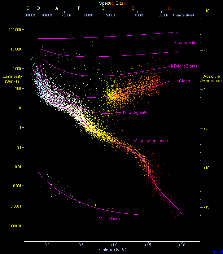
Fig. 4.5 An observational Hertzsprung–Russell diagram with 22,000 stars plotted from the Hipparcos Catalogue and 1,000 from the Gliese Catalogue of nearby stars. Image credit: Wikipedia by Richard Powell.

The Sun (G2) is found on the main sequence of the H-R diagram, which has both axes scaled logarithmically to accommodate the huge span of stellar luminosities and temperatures. The main sequence is not a straight line, but a curve with a finite width due to changes in the star’s temperature and luminosity that occur over its main sequence lifetime. The giants occupy the region above the main sequence, where the brightest stars are supergiants and can occupy a range in spectral type (e.g., blue or red supergiants). After converting spectral type to surface temperature and absolute magnitude to luminosity, Eqn. (4.13) can be used to determine the radius of a star. If two stars have the same surface temperature, but one stars is 100 times brighter than the other, then the radius of the brighter star is \(\sqrt{100}=10\) times larger. A logarithmically scaled H-R diagram allows for lines of constant radius since the Stefan-Boltzmann law is represented as a power law.

The existence of a simple relation between the luminosity and temperature for main=sequence stars is a valuable clue that the star’s mass plays an important role in determining when a star lies on the main sequence. The H-R diagram spans from the most massive O stars (\(60\; M_\odot\)) to the least massive M stars (\(0.08\;M_\odot\)). Knowing both the mass and radius of stars allows for the calculation of the average density of the stars. Surprisingly, main-sequence stars have roughly the same density as water and moving up the main sequence, the more massive, larger, early type stars have a lower average density.

Exercise 4.5

What is the average density of the Sun?

The average density of the Sun is calculated given the Sun’s mass (\(M_\odot = 1.9891 \times 10^{30}\ {\rm kg}\)) and radius (\(R_\odot = 6.95508 \times 10^8\ {\rm m}\)) using the equation for density \(\bar{\rho} = {\rm M/V}\). The average density of the Sun is

\[\begin{align*} \bar{\rho}_\odot = \frac{1.9891 \times 10^{30}\ {\rm kg}}{\frac{4}{3}\pi \left( 6.95508 \times 10^8\ {\rm m}\right)^3} = 1410\ {\rm kg/m^3}. \end{align*}\]

Exercise 4.6

How do the stars Sirius A and Betelgeuse compare to the Sun in terms of average density?

Having calculated the average density of the Sun in the previous problem, we can use measurments of other stars in solar units to determine the relative average density of those stars. The average density of Sirius A and Betelguese are

\[\begin{align*} \rho_{\rm Sirius\ A} &= \frac{2.063\ M_\odot}{\frac{4}{3}\pi \left(1.711\ R_\odot \right)^3} = \frac{2.063}{1.711^3} \bar{\rho}_\odot, \\ & = 0.412\bar{\rho}_\odot = 581.3\ {\rm kg/m^3}, \\ \\ &\quad \text{and} \\ \\ \rho_{\rm Betelgeuese} &= \frac{16.5\ M_\odot}{\frac{4}{3}\pi \left(1021\ R_\odot \right)^3}= \frac{16.5}{1021^3} \bar{\rho}_\odot, \\ & = 1.55 \times 10^{-8} \bar{\rho}_\odot = 2.188 \times 10^{-5}\ {\rm kg/m^3}. \end{align*}\]

def avg_stellar_density(M,R):
    #M = stellar mass in M_sun
    #R = stellar radius in R_sun
    rho = M/R**3
    rho_SI = (M*M_sun)/(4./3.*np.pi*(R*R_sun)**3)
    return rho, rho_SI

M_sun = 1.9891e30 #kg; conversion factor for M_sun --> kg
R_sun = 6.95508e8 #m; conversion factor for R_sun --> m

rho_sun, rho_sun_SI = avg_stellar_density(1,1)
print("The average stellar density of the Sun is %1.1f rho_odot or %1.2e kg/m^3." % (rho_sun,rho_sun_SI))

rho_Sirius, rho_Sirius_SI = avg_stellar_density(2.063,1.711)
print("The average stellar density of Sirius A is %1.3f rho_odot or %1.3e kg/m^3." % (rho_Sirius,rho_Sirius_SI))

rho_Betelgeuse, rho_Betelgeuse_SI = avg_stellar_density(16.5,1021) #adopting lowest mass estimate and maximum radius
print("The average stellar density of Betelgeuse is %1.3e rho_odot or %1.3e kg/m^3." % (rho_Betelgeuse,rho_Betelgeuse_SI))

The average stellar density of the Sun is 1.0 rho_odot or 1.41e+03 kg/m^3.
The average stellar density of Sirius A is 0.412 rho_odot or 5.813e+02 kg/m^3.
The average stellar density of Betelgeuse is 1.550e-08 rho_odot or 2.188e-05 kg/m^3.

Table 4.3 provides the the average stellar density \(\bar{\rho}\) of the Sun, Sirius A, and Betelgeuse. The Sun is 41% more dense (on average) than water (\(\rho_{\rm water} = 1000\;{\rm kg/m^3}\)), while Sirius A and Betelgeuse are less dense than water. This implies that more massive stars would float in water!

Table 4.3 Average Stellar Density of the Sun, Sirius A, and Betelgeuse.

Star	\(M\) (\(M_\odot\))	\(R\) (\(R_\odot\))	\(\bar{\rho}\) (\(\rho_\odot\))	\(\bar{\rho}\;{\rm kg/m^3}\)
Sun	\(1.0\)	\(1.0\)	\(1.0\)	\(1410\)
Sirius A	\(2.063 \)	\(1.711\)	\(0.412\)	\(581.3\)
Betelgeuse	\(16.5\)	\(1021\)	\(1.55 \times 10^{-8}\)	\(2.19 \times 10^{-5}\)

4.2.2. Morgan-Keenan Luminosity Classes

Using the spectra cataloged by Antonia Maury, Hertzsprung found a difference in the spectra of giant and main-sequence stars of the same spectral type. There are subtle differences in the relative strengths of spectral lines for stars of similar effective temperatures and different luminosities. In 1943, William W. Morgan, Phillip C. Keenan, and Edith Kellman published the Atlas of Stellar Spectra, which consists of 55 prints of spectra that clearly display the effect of temperature and luminosity. The MKK Atlas established the 2D Morgan-Keenan (M-K) system of spectral classification.

A luminosity class is appended to a star’s Harvard spectral type and designated by a Roman numeral (see Table 4.4). The supergiant stars use the Roman numeral “I” (also divided into subclasses Ia and Ib), where main-sequence stars use the Roman numeral “V”. The strengths of two closely spaced lines are measured and their ratio is often used to place a star in the appropriate luminosity class. In general, narrower lines are usually produced by more luminous stars with the same spectral type. The series of Roman numerals extends below the main sequence, where the subdwarfs (VI or “sd”) are slightly to the left of the main sequence because they are deficient in metals. The M-K system is not applied to white dwarfs, which are instead classified by the letter D.

The 2D M-K classification scheme enables astronomers to locate a star’s position on the H-R diagram based entirely on the appearance of its spectrum. Using a star’s absolute magnitude M (see the magnitude scale) from the vertical axis of the H-R diagram, the distance to the star can be calculated from its apparent magnitude m. This method of distance determination is called the spectroscopic parallax and is responsible for many of the measured stellar distances. The accuracy of spectroscopic parallax is limited because there is not a perfect correlation between the absolute magnitude and luminosity class. A specific luminosity class has an intrinsic scatter of about \(\pm 1\) magnitude, which corresponds to a brightness difference of \(10^{1/5}\) or 1.6.

Note

Since the technique of parallax is not involved, the term spectroscopic parallax is a misnomer. Although, the name does give a connotation of distance determination.

Table 4.4 Morgan-Keenan Luminosity Classes.

Class	Type of Star
Ia-O	Extreme, luminous supergiants
Ia	Luminous supergiants
Ib	Less luminous supergiants
II	Bright giants
III	Normal giants
IV	Subgiants
V	Main-sequence (dwarf) stars
VI, sd	Subdwarfs
D	White dwarfs

4.3. Homework

Problem 1

For a gas of neutral hydrogen atoms, at what temperature is the number of atoms in the 1st excited state only 1% of the number of atoms in the ground state? What is the temperature for 10%?

Problem 2

The partition function (Eqn. (4.7)) actually diverges for \(n\rightarrow \infty\). Why can we ignore these large \(n\) terms?

Problem 3

Assuming an stellar atmosphere composed of pure helium (which is actually a white dwarf), you want to find the temperature at the middle of the He I partial ionization zone, where half of the He I atoms have been ionized. The ionization energies of neutral helium and singly ionized helium are \(\chi_{\rm I} = 24.6\) eV and \(\chi_{\rm II} = 54.4\) eV, respectively. The partition functions are \(Z_{\rm I} = 1\), \(Z_{\rm II} = 2\), and \(Z_{\rm III} = 1\). Use \(P_e = 20\;{\rm N/m^2}\) for the electron pressure.

(a) Use Eqn. (4.8) (with a substitution for the electron pressure \(P_e\)) to find \(N_{\rm II}/N_{\rm I}\) and \(N_{\rm III}/N_{\rm II}\) for temperatures 5000 K, 15,000 K, and 25,000 K. How do they compare?

(b) Show that \(N_{\rm II}/N_{\rm total} = N_{\rm II}/(N_{\rm I}+N_{\rm II}+N_{\rm III})\) can be expressed in terms of the ratios \(N_{\rm II}/N_{\rm I}\) and \(N_{\rm III}/N_{\rm II}\).

(c) Make a graph of \(N_{\rm II}/N_{\rm total}\) for a range of temperatures 5000 K to 25,000 K. What is the temperature at the middle of the He I partial ionization zone?

Problem 4

Use the Saha equation to determine the fraction of hydrogen atoms that are ionized, \(N_{\rm II}/N_{\rm total}\) at the center of the Sun. Here the temperature is \(15.7 \times 10^6\) K and the number density of electrons is about \(n_e = 6.1 \times 10^{31}\;{\rm m^{-3}}\). Does your result agree with the fact that practically all of the Sun’s hydrogen is ionized at the Sun’s center? What is the reason for any discrepancy?

Problem 5

A white dwarf star typically has a radius that is only 1% of the Sun’s. Determine the average density of a Solar-mass white dwarf.

Problem 6

Fomalhaut A has an apparent visual magnitude of \(V = 1.16\) and has a surface temperature of 8590 K (or \(B-V = 0.09\)). Use the H-R diagram to determine the distance to this star.