The Fate of Massive Stars

11. The Fate of Massive Stars#

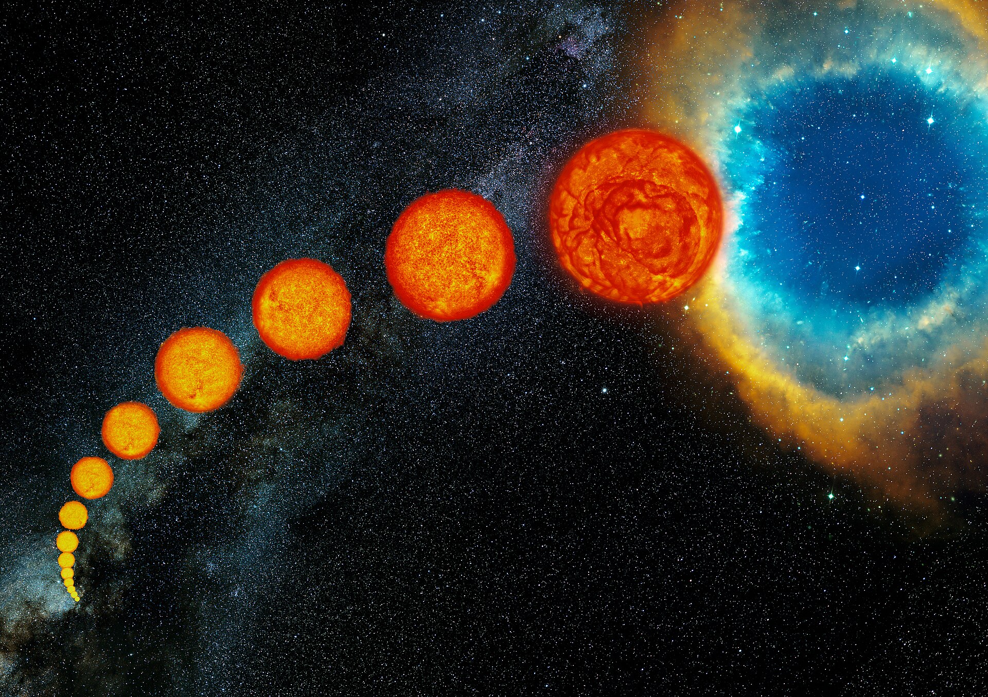
11.1. Post-Main-Sequence Evolution of Massive Stars#

Since at least 1600, astronomers have observed $\eta$ Carinae, where its apparent magnitude was reported to be either 2 or 4. In the early 1800s, it may have become significantly more active. In 1837, $\eta$ Car suddenly brightened, fluctuating in magnitude between $0-1$ and made it the second brightest object in the sky (only Sirius was brighter). This brightening event is remarkable because the star is approximately 2300 pc from Earth, where Sirius is only 2.64 pc away.

After 1856, $\eta$ Car began to fade and dropped in magnitude to 8 by 1870. Since 1895, $\eta$ Car has been relatively quiet and it has brightened slightly to a magnitude 6 over the past ~150 years. In a similar fashion, P Cygni was too faint to see with the naked eye before 1600, but suddenly brightened to a magnitude 3. Following this event, P Cyg faded for a time and reappeared in 1655 becoming nearly as bright as it was in 1600. Since 1700, P Cyg has been a magnitude 5 star, although it may have brighten slightly over the past several centuries.

11.1.1. Luminous Blue Variables#

A small number of other stars in our own galaxy (some farther away) behave like $\eta$ Car and P Cyg. For example S Doradus (located in the Large Magellanic Cloud) is the best known extragalactic example. Similar stars were discovered by Edwin Hubble and Allan Sandage, where this class of star are referred to as S Doradus variables, Hubble-Sandage variables, and luminous blue variables (LBVs).

An extreme example of an LBV is $\eta$ Car, where it is known as the “homunculus” for its bipolar structure and equatorial disk. From Doppler measurements, the lobes of $\eta$ Car expand outward at $650\ {\rm km/s}$ and a range of velocities are recorded along any particular line-of-sight. The expanding lobes are hollow, while the material in the shells contain molecules of ${\rm H_2}$, ${\rm CH}$, and ${\rm OH}$. It appears that the homunculus is significantly depleted in ${\rm C}$ and ${\rm O}$, while enriched in ${\rm He}$ and ${\rm N}$. This suggests that the ejected material has been processed by the CNO cycle. The present mass loss rate of $\eta$ Car is $\sim 10^{-3}\ M_\odot/{\rm yr}$, but it has probably ejected $1-3\ M_\odot$ during the 20 years following the Great Eruption of 1837.

During the Great Eruption, $\eta$ Car’s luminosity could have been $4\times$ brighter than its present quiescent luminosity ($\sim 5\times10^6\ {\rm L_\odot}$). The central star’s effective temperature is roughly 30,000 K. As of 2007, the apparent magnitude in the visual was $m_V \sim 6$, but now (2018) it has brightened to $m_V \sim 4.3$. Most of $\eta$ Car’s luminosity is initially emitted in the UV, which explains its high effective temperature. Much of the UV is scattered, absorbed, and re-emitted by dust grains into the IR.

As a class, LBV’s tend to have high effective temperatures (15,000-30,000 K), with luminosities greater than $10^6\ {\rm L_\odot}$. As a result, LBVs are in the upper left-hand portion of the H-R diagram. LBVs are clearly evolved, post-main-sequence stars given the composition of their atmospheres and ejecta. LBVs also cluster in an instability region of the H-R diagram, which suggests that their behavior is transient.

A variety of mechanisms were proposed to explain the variability and dramatic mass loss of LBVs. the upper end of the main sequence is very near the Eddington luminosity limit where the force due to the radiation pressure may equal of exceed the gravitational force on the outer surface layers of a star. The derived expression for the Eddington luminosity limit is

\[ L_{{\rm ED}} = \frac{4\pi Gc}{\kappa}M, \]

which depends on the opacity $\kappa$ and stellar mass $M$. The “classical” Eddington limit assumes that the opacity is solely due to the scattering of free electrons, which is constant $\sigma_T$ for a completely ionized gas. A “modified” Eddington limit was proposed by Humphreys & Davidson (1994), where some temperature-dependent factor of opacity modifies the overall opacity as the star evolves to the right in the H-R diagram. As the temperature decreases and the opacity increases, the Eddington luminosity would drop below the actual luminosity of the star. This implies that the radiation pressure dominates over gravity, which drives mass loss from the envelope.

A second suggestion is that atmospheric pulsation instabilities may develop, like Cepheids, RR Lyrae, long-period variable stars. Also intriguing is the apparent high rotation velocity of some LBVs. Rapid rotation would result in decreasing the “effective” gravity at the equator due to centrifugal effects and allow for gases to be driven away from the surface at the equator. The disk around $\eta$ Car may have formed from a high spin during the lesser eruption between 1887-1895.

LBVs could also be members of binary star systems as similar behaviors can be induced by the binary companion. Interestingly, $\eta$ Car exhibits a 5.54 yr periodicity in the equivalent widths (of some) of its spectral lines, which hints at the presence of a binary companion. Although it is unclear how a binary companion can cause all of the effects observed. It may turn out that more than one of the discussed mechanisms could influence the behavior of the LBVs or the principal mechanism has yet to be identified.

11.1.2. Wolf-Rayet Stars#

Closely related to LBVs are the Wolf-Rayet (WR) stars, which were first discovered by Charles Wolf and Georges Rayet while working at the Paris Observatory in 1867. Using a visual-wavelength spectrometer to conduct a survey of stars in Cygnus, they observed three stars (within one degree of each other) that exhibited strong, very broad emission lines rather than the typical absorption lines observed in other stars. Today 220+ WR stars have been identified in the Milky Way, although the total number of WRs is estimated to be 1000-2000 on the basis of sampling statistics.

Along with strong emission lines, WR stars are very hot, with effective temperatures of $25,000-100,000\ {\rm K}$. WRs are also losing mass ($>10^{-5}\ M_\odot/{\rm yr}$) with wind speeds from $800-3000\ {\rm km/s}$. There is strong evidence that many (perhaps all) WR stars are rapid rotators with equatorial speeds of $\sim 300\ {\rm km/s}$. LBVs are all very massive stars ($85\ M_\odot$), but WRs can have progenitor masses as low as $20\ M_\odot$. Also, WRs do not demonstrate the dramatic variability that is characteristic of LBVs.

As mentioned previously, the unusual spectra really sets WR stars apart from other stars. The spectra also reveal a spectra that we today recognize as three classes: WN, WC, and WO.

WNs are dominated by emission lines of helium and nitrogen, although emission from carbon, oxygen, and hydrogen is detectable in some cases.
WCs exhibit emission lines of helium and carbon, with a distinct absence of nitrogen and hydrogen lines.
WOs are much rarer than either WNs or WCs. They have spectra containing prominent oxygen lines, with some contribution from highly ionized species.

WN and WC stars are further subclassified based on the degree of ionization in their atmospheres. They are also classified as “early” (E) or “late” (L). For example, for the WN stars:

WN2 stars show spectral lines of ${\rm He\ II}$, ${\rm N\ IV}$, and ${\rm O\ VI}$.
WN9 stars contain spectra of low-ionization species, such as ${\rm He\ I}$ and ${\rm N\ III}$.
WNE stars are Wolf-Rayet stars of ionization classes WN2-WN5.
WNL stars are ionization classes WN6-WN11.

and for the WC stars:

WC4 stars have higher ionization levels (${\rm He\ II,\ O\, IV,\ C\ VI}$)
WC9 stars exhibit lower ionization levels, such as ${\rm He\ I}$ and ${\rm C\ II}$
WCEs range from WC4-WC6
WCLs range from WC7-WC9

A trend in composition from WN $\rightarrow$ WC $\rightarrow$ WO was eventually recognized as a direct consequence of the stellar mass loss. WNs have lost virtually all of their hydrogen-dominated envelopes, which reveals the material synthesized by nuclear reactions in the core. Core convection brings material to the surface that has been processed by the CNO cycle. Additional mass loss results in the ejection of the CNO processed material, which exposes the helium-burning material generated by the triple alpha process. If the star survives long enough, mass loss will eventually strip away all but the oxygen component of the triple-alpha ash.

In addition to LBVs and WRs, the upper portion of the H-R diagram also contains blue supergiants (BSG), red supergiants, and Of stars (O supergiants with pronounced emission lines).

11.1.3. A General Evolutionary Scheme for Massive Stars#

A general evolution path for massive stars has been outline, where the scheme was originally suggested by Peter Conti and subsequently modified. In each case the star ends its life in a supernova (SN) explosion. Note that the masses listed below oar only approximate (Massey (2003)).

\[\begin{split}\begin{align*} M > 85\ M_\odot &: {\rm O} \rightarrow {\rm Of} \rightarrow {\rm LBV} \rightarrow {\rm WN} \rightarrow {\rm WC} \rightarrow {\rm SN} \\ 40\ M_\odot < M < 85\ M_\odot &: {\rm O} \rightarrow {\rm Of} \rightarrow {\rm WN} \rightarrow {\rm WC} \rightarrow {\rm SN} \\ 25\ M_\odot < M < 40\ M_\odot &: {\rm O} \rightarrow {\rm RSG} \rightarrow {\rm WN} \rightarrow {\rm WC} \rightarrow {\rm SN} \\ 20\ M_\odot < M < 25\ M_\odot &: {\rm O} \rightarrow {\rm RSG} \rightarrow {\rm WN} \rightarrow {\rm SN} \\ 10\ M_\odot < M < 20\ M_\odot &: {\rm O} \rightarrow {\rm RSG} \rightarrow {\rm BSG} \rightarrow {\rm SN} \\ \end{align*} \end{split}\]

This qualitative evolutionary scheme is supported by detailed numerical evolutionary models of massive star formation. Evolutionary tracks for stars of solar composition are calculated for the range from $9-120\ M_\odot$. The models can be modified if the include the effects of the equatorial rotation, which have appreciable effects on driving internal mixing and enhancing mass loss as part of the stellar evolution.

11.1.4. The Humphreys-Davidson Luminosity Limit#

The massive-star evolutionary tracks indicate that the most massive stars never evolve to the red supergiant (RSG) portion of the H-R diagram. This is consistent with observations. Humphreys and Davidson first pointed out the there is an upper-luminosity cut-off in the H-R diagram that includes a diagonal component running from highest luminosities and effective temperatures to lower values in both parameters. When full redward evolutionary tracks develop for stars below $\sim 40\ M_\odot$, the Humphreys-Davidson luminosity limit continues at constant luminosity.

Very massive stars are extremely rare (only one $100\ M_\odot$ star exists for every one million solar mass stars), but they play a major role in the dynamics and chemical evolution of the ISM. The tremendous amount of kinetic energy deposited in the ISM through the stellar winds of massive stars has an impact on the kinematics of the ISM. When very massive stars form, they have the ability to quench (stop) star formation in neighboring regions. The UV light from massive stars can also ionize gas clouds around them. The highly enriched gases of massive stellar winds increase the metal content of the ISM, resulting in the formation of increasingly metal-rich stars.

https://github.com/saturnaxis/ModernAstro/blob/main/Chapter_15/Figure_3.jpg?raw=true? — Fig. 11.3 The evolution of massive stars with $Z=0.02$. The solid lines are evolutionary tracks with initial rotation velocities of $300\ {\rm km/s}$ and the dotted lines are tracks for stars without rotation. (Carroll & Ostlie (2007); Figure from Meynet & Maeder, Astron. Astrophys., 404, 975, 2003.)#

11.2. The Classification of Supernovae#

In 1006, an extremely bright star suddenly appeared in the constellation Lupus, which reached an estimated visual magnitude of $m_V = -9$ and it was reportedly bright enough to read by at night (compared to a full Moon, $m_V = -12.5$, which is $\sim 25\times$ brighter). The event was recorded by astrologers across Europe, China, Japan, Egypt, and Iraq. Based on their writings, the bright star appeared bout April 30, 1006 and faded from view roughly one year later. Today, this event is called Supernova 1006 (SN 1006).

Note

A very small number of supernovae have been recorded from historical writings more than 2000 years ago. When a supernova date or year is given, it is most likely referring to A.D. or CE.

Other similar events have been recorded through human history, although they are rare. Only 48 years after the 1006 event, a “guest star” appeared in the constellation Taurus. Yang Wei-T’e, a court astrologer during China’s Sung dynasty, recorded the event and noted that after more than a year it gradually became invisible. The star was also noted by the Japanese, Koreans, and Arabs (appearing in an Arabic medical textbook). The Europeans may have witnessed the event as well, but the evidence is unclear. Like the previous event, the amazing star was visible during daylight (like the Moon is at times). Modern astronomers have identified a rapidly expanding cloud, which is the reported location of the ancient “guest star” and is known as the Crab supernova remnant.

Another star suddenly appeared in the heavens about 500 years later that was witnessed by Tycho Brahe in 1572. The strange occurrence was clearly in contrast to the Western belief that the heavens were unchanging. Johannes Kepler also witnessed a supernova explosion in 1604, where these two events are now known as Tycho’s supernova and Kepler’s supernova.

Kepler’s supernova was the last observed supernova to occur in the Milky Way. On February 24, 1987 at 23 UT, Ian Shelton detected SN 1987A just southwest of a massive molecular cloud region in the Large Magellanic Cloud (LMC) known as 30 Doradus; the observation was made with a 10-inch astrograph (Newtonian reflector) at Las Campanas Observatory in Chile. The LMC is a dwarf galaxy and only 50 kpc from Earth. It was quickly realized that the progenitor of the supernova was a blue supergiant (BSG) star. Nicholas Sanduleak had cataloged the star Sk -69 202 while investigating hot stars in the Magellanic Clouds.

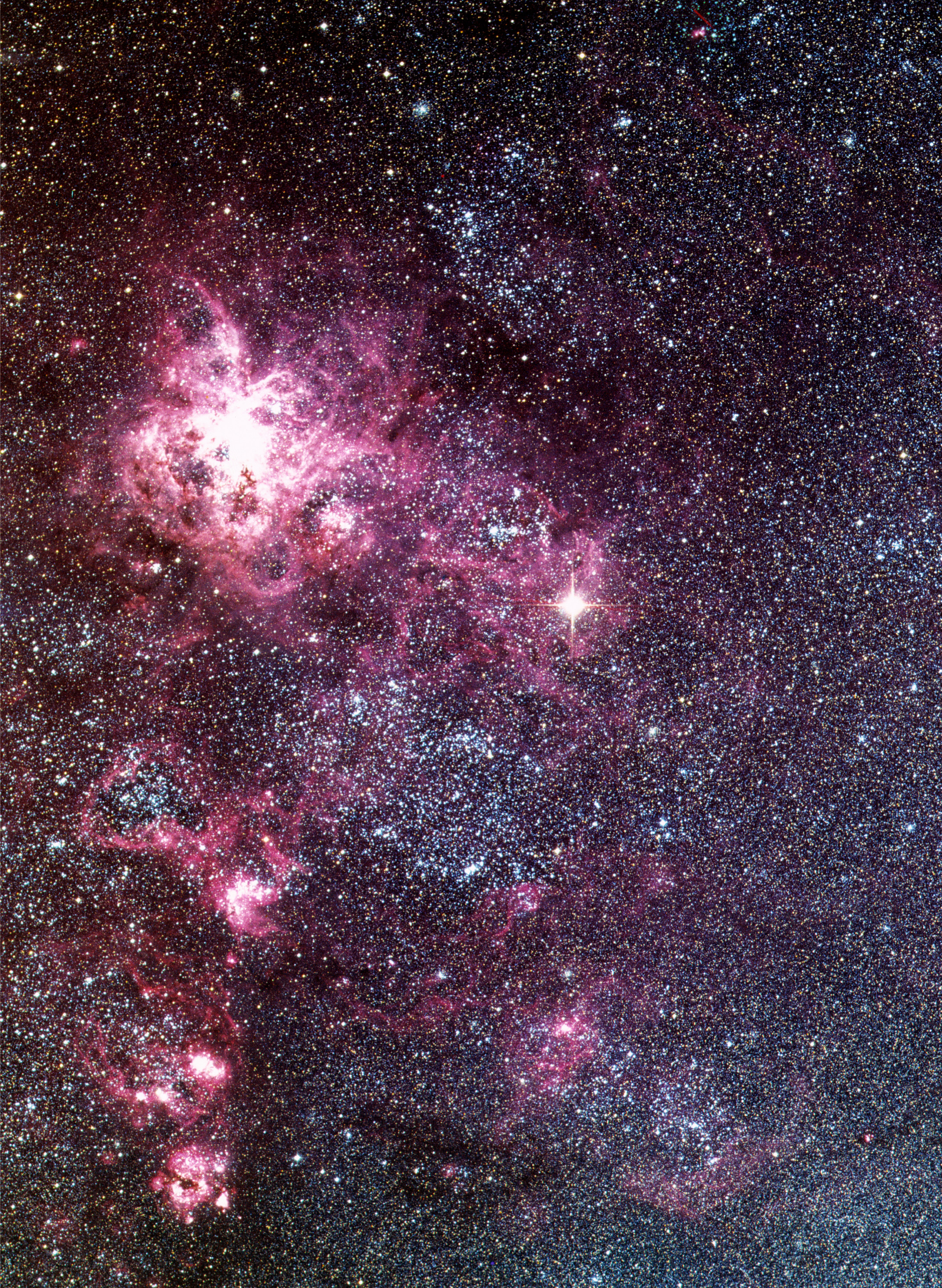
https://cdn.eso.org/images/large/eso0708a.jpg — Fig. 11.5 A portion of the Large Magellanic Cloud showing SN 1987A. (Carroll & Ostlie (2007); Image Credit: ESO)#

11.2.1. Classes of Supernovae#

Today, astronomers routinely observe supernovae in other galaxies, where the “A” in SN 1987A represents the first supernova reported that year. However, supernovae are exceedingly rare events, which typically occur about once very 100 years in any one galaxy. There are many galaxies to study and over time, it has been realized that there are several distinct classes of supernovae with different classes of underlying progenitors and mechanisms.

Type I supernovae were identified as those without any hydrogen lines in their spectra. Given that hydrogen is the most abundant element, this was an indication of something unusual. These supernovae are further subdivided according to their spectra.
- Type Ia show a strong ${\rm Si\ II}$ line at 615 nm.
- Type Ib or Ic are classified by the respective presence or absence of strong helium lines.
Type II supernovae contain strong hydrogen lines, in contrast to the Type I supernovae.
- Type II-L show a linear decrease in the apparent magnitude $m_B$ after the maximum.
- Type II-P show a plateau between 30-80 days in the apparent magnitude $m_B$ after the maximum. Type II-P supernovae occur approximately 10 times more often than Type II-L supernovae.

The lack of hydrogen lines in Type I supernovae indicates that the progenitor stars were stripped of their hydrogen envelopes. The differences in the spectral signatures between each Type I (a, b, or c) indicate that different physical mechanisms are at work. Type Ia are found in all types of galaxies, including ellipticals that show very little evidence of recent star formation (e.g., ${\rm H\ II}$ regions). Short-lived, massive stars are probably involved with Types Ib and Ic (to expose or get rid of the excess helium), but not with Type Ia.

Supernova Spectra

https://github.com/saturnaxis/ModernAstro/blob/main/Chapter_15/Figure_6.jpg?raw=true? — Fig. 11.6 Representative spectra of the four types of supernovae: Type Ia, Ib, Ic, and II. Brightness is in arbitrary flux units. (Carroll & Ostlie (2007); Image Credit: Thomas Matheson, NOAO)#

Type Ia in Blue

https://github.com/saturnaxis/ModernAstro/blob/main/Chapter_15/Figure_7.jpg?raw=true? — Fig. 11.7 Composite light curve for Type I supernova at blue wavelengths. (Carroll & Ostlie (2007); Figure adapted from Doggett & Branch, Astron. J. 90, 2303, 1985)#

The typical peak brightness of a Type Ia is $M_B = -18.4$, while the light curves of Types Ib and Ic are fainter by 1.5-2 magnitudes (in blue light). All Type I supernovae show similar rates of decline of their brightness after the maximum with a decline of $0.065 \pm 0.007$ magnitude per day at 20 days. After about 50 days the dimming slows and becomes constant, where a Type Ia declines 50% faster $(0.015\ {\rm mag/day})$ than the other Type Is $(0.010\ {\rm mag/day})$. It is believed that SN 1006, Tycho (SN 1572), and Kepler (Sn 1604) were all Type I.

Observationally, Type II supernovae are characterized by a rapid rise in luminosity and reach a maximum brightness that is typically 1.5 magnitudes dimmer than a Type Ia. The peak light output is followed by a steady decrease, which drops 6-8 magnitudes in a year. Their spectra also exhibit lines associate with hydrogen and heavier elements. P Cygni profiles are common in many lines, which indicates rapid expansion. The Crab supernova (SN 1054) and SN 1987A were Type II.

Nature loves to confound our clean classification schemes, where SN 1993J (in M81) initially displayed strong hydrogen emission lines and follows the Type II scheme. Within a month the hydrogen lines were replaced by helium and its appearance changed to a Type Ib. This suggests that Type Ib and Type II supernovae are related in some way.

Supernova Light Curve Shapes

https://github.com/saturnaxis/ModernAstro/blob/main/Chapter_15/Figure_8.jpg?raw=true? — Fig. 11.8 The characteristic shapes of Type II-P and Type II-L light curves. These are composite light curves based on observations of many supernovae. (Carroll & Ostlie (2007); Figure adapted from Doggett & Branch, Astron. J. 90, 2303, 1985)#

Supernova Classification

https://github.com/saturnaxis/ModernAstro/blob/main/Chapter_15/Figure_9.jpg?raw=true? — Fig. 11.9 The classification of supernovae based on their spectra at maximum light and the existence or absence of a plateau in the Type II light curve. (Carroll & Ostlie (2007))#

11.3. Core-Collapse Supernovae#

The sheer amount of energy released in a supernova event is staggering, where a typical Type II releases $10^{46}\ {\rm J}$, with about 1% of that appearing as kinetic energy of the ejected material and less than 0.01% being released as the photons that produce the spectacular visual display. The remainder of the energy is radiated in the form of neutrinos.

Exercise 11.1

How much iron could ultimately be produced through a typical Type II supernova explosion?

A typical Type II supernova releases $10^{46}\ {\rm J}$. Converting this energy into a rest mass through $E= mc^2$, we get

\[ m = \frac{E}{c^2} = 10^{46}\ \frac{\rm J}{c^2} = 1 \times 10^{29}\ {\rm kg} = 0.06 M_\odot. \]

The binding energy of an iron-56 nucleus $({\rm ^{56}_{26} Fe})$ is 492.26 MeV and the mass of the nucleus is $55.934939\ {\rm u}$. If all the energy of a Type II went into the formation of iron nuclei, it would be necessary to form

\[ N = \left( \frac{10^{46}\ {\rm J}}{492.26\ {\rm MeV/nucleus}} \right) \left( \frac{1\ {\rm MeV}}{1.6 \times 10^{-13}\ {\rm J}} \right) = 1.3 \times 10^{56}\ {\rm nuclei}, \]

which corresponds to a mass of iron of

\[ m = \left(1.3 \times 10^{56}\ {\rm nuclei}\right)\left(55.934939\ {\rm u} \right) \left(1.66 \times 10^{-27}\ {\rm kg/u} \right) = 1.2 \times 10^{31}\ {\rm kg} = 5.9\ M_\odot. \]

Actually, iron is not formed as a result of releasing the energy involved in a supernova explosion, where the energy source is not nuclear. However, iron is critically involved in the process.

from scipy.constants import c, e

M_Sun = 1.989e30 #solar mass in kg
MeV = 1e6*e #MeV in Joules

Type_II_Energy = 1e46 #energy released in a Type II in J
rest_mass = Type_II_Energy/c**2

print("The rest mass of a Type II is %1.0e or %1.2f M_Sun." % (rest_mass,rest_mass/M_Sun))

N_Fe = Type_II_Energy/492.26/MeV 
print("The number of iron nuclei produced from 10^46 J of energy is %1.1e nuclei" % N_Fe)

m_Fe = N_Fe*55.934939*1.66e-27
print("The total mass of iron produced from 10^46 J of energy is %1.1e kg or %1.1f M_Sun." % (m_Fe,m_Fe/M_Sun))

The rest mass of a Type II is 1e+29 or 0.06 M_Sun.
The number of iron nuclei produced from 10^46 J of energy is 1.3e+56 nuclei
The total mass of iron produced from 10^46 J of energy is 1.2e+31 kg or 5.9 M_Sun.

11.3.1. Core-Collapse Supernova Mechanism#

The post-main-sequence evolution of stars more massive than about $8\ M_\odot$ is different. Hydrogen is converted into helium on the main sequence and is followed by helium burning that leads to a carbon-oxygen core. The very high temperature in the core of a massive star means that carbon and oxygen can burn as well. The end result is that rather than the star ending its life through the formation of a planetary nebula, a catastrophic supernova explosion occurs instead.

The details of supernovae are continually being worked out, but the story of how they are produced is becoming clearer. The three types (Type Ib, Ic, and II) are closely related and involve the collapse of a massive, evolved stellar core. Collectively, these supernovae are known as core-collapse supernovae.

As the helium-burning shell continues to add ash to the carbon-oxygen core (and as the core contracts), it eventually ignites in carbon burning and generates a variety of by-products (e.g., ${\rm ^{16}_8 O}$, ${\rm ^{23}_{11} Na}$, ${\rm ^{23}_{12} Mg}$, and ${\rm ^{24}_{12} Mg}$). This leads to a succession of nuclear reaction sequences that depend sensitively on the stellar mass.

Assuming that reach reaction sequence develops an equilibrium, an “onion-like” shell structure develops in the stellar interior. Following carbon burning, the oxygen in the ${\rm Ne-O}$ core will ignite, which produces a new core composition dominated by silicon-28. Finally at temperatures near $3 \times 10^9\ {\rm K}$, silicon burning can commence through a series of reactions, such as

\[\begin{split}\begin{align*} {\rm ^{28}_{14} Si} + {\rm ^4_2 He} &\rightleftharpoons {\rm ^{32}_{16} S} + \gamma \\ {\rm ^{32}_{16} S} + {\rm ^4_2 He} &\rightleftharpoons {\rm ^{36}_{18} Ar} + \gamma \\ & \vdots \\ {\rm ^{52}_{24} Cr} + {\rm ^4_2 He} &\rightleftharpoons {\rm ^{56}_{28} Ni} + \gamma. \end{align*} \end{split}\]

Silicon burning produces a host of nuclei centered near the iron-56 peak of the binding energy per nucleon curve. The most abundant end products are probably iron-54, iron-56, and nickel-56. Any further reactions that produce more massive nuclei (than iron-56) are endothermic and cannot contribute to the luminosity of the star. Grouping all the products together, silicon burning produces an iron core.

https://github.com/saturnaxis/ModernAstro/blob/main/Chapter_15/Figure_10.jpg?raw=true? — Fig. 11.10 The onion-like interior of a massive star that has evoled through core silicon burning. This drawing is not to scale. (Carroll & Ostlie (2007))#

Carbon, oxygen, and silicon burning produce nuclei with masses progressively nearer the iron peak of the binding energy curve, which means that less and less energy is generated per unit mass of fuel. The timescale for each succeeding reaction sequence becomes shorter. For a $20\ M_\odot$ star

the main-sequence lifetime (core hydrogen burning) is roughly $10^7$ years , where
helium burning requires $10^6\ {\rm yr}$,
carbon burning lasts $300\ {\rm yr}$,
oxygen burning takes around $200\ {\rm days}$, and
silicon burning is complete in only $2\ {\rm days}$.

At the very high temperature now present in the core, the photons possess enough energy to destroy heavy nuclei, which is known as photodisintegration (note the reverse arrows in the silicon burning sequence). Particularly important are the reactions that photodisintegrate iron-56 and helium-4:

\[\begin{split} \begin{align*} {\rm ^{56}_{26} Fe} + \gamma &\rightarrow 13\ {\rm ^4_2 He} + 4n \\ {\rm ^4_2 He} + \gamma &\rightarrow 2 p^+ + 4n. \end{align*} \end{split}\]

When the mass of the contracting iron core has become large enough (and the temperature sufficiently high), photodisintegration can undo what the star has been trying to do for its entire life in a very short period of time, namely produce elements more massive than hydrogen and helium. This process of stripping iron down to individual protons and neutrons is highly endothermic (i.e., thermal energy is removed from the gas that otherwise would be supporting the core of the star). The core masses for which this process occurs vary from $1.3\ M_\odot$ for a $10\ M_\odot$ ZAMS star to $2.5\ M_\odot$ for a $50\ M_\odot$ star.

Under the extreme conditions (e.g., $T_c \sim 8\times 10^9\ {\rm K}$ and $\rho_c \sim 10^{13}\ {\rm kg/m^3}$ for a $15\ M_\odot$ star), the free electrons that supported the star through degeneracy pressure are captured by heavy nuclei and the protons produced by photodisintegration; for instance,

\[ p^+ + e^- \rightarrow n + \nu_e. \]

The amount of energy that escapes the star in the form of neutrinos becomes enormous. The photon luminosity of a $20\ M_\odot$ stellar model is $4.4 \times 10^{31}\ {\rm W}$, while the neutrino luminosity is $3.1 \times 10^{38}\ {\rm W}$.

Through the photodisintegration of iron (combined with the electron capture by protons and heavy nuclei) most of the core’s support is suddenly gone (i.e., no electron degeneracy pressure) and the core begins to collapse extremely rapidly. The collapse is homologous in the inner portion of the core and collapse velocity scales with the distance away from the stellar center.

At the radius where the velocity exceeds the local sound speed, the collapse can no longer remain homologous and the inner core decouples from the now supersonic outer core, which is left behind and nearly in free-fall. During the collapse, speeds in the outer core can reach almost $70,000\ {\rm km/s}$ and within about on second an Earth-sized volume can be compressed down to a radius of $50\ {\rm km}$.

Exercise 11.2

If an Earth-sized mass collapses to a radius of $50\ {\rm km}$, a tremendous amount of gravitational potential energy would be released. Can this energy be responsible for the energy of a core-collapse supernova?

From the virial theorem, the potential energy of a spherically symmetric star of constant density is

\[ U = - \frac{3}{5} \frac{GM^2}{R}. \]

Equating the potential energy U released during the collapse to the energy from a Type II supernova, $E_{II} = 10^{46}\ {\rm J}$, and given that the final radius $R_f$ is 50 km, the amount of mass required to produce the supernova would be

\[ M \simeq \sqrt{\frac{5}{3}\frac{E_{II}R_f}{G}} \simeq 4 \times 10^{30}\ {\rm kg} \simeq 1.8\ M_\odot. \]

This value is within the range $1.3-2.5\ M_\odot$ given earlier.

from scipy.constants import G
import numpy as np

M_Sun = 1.989e30 #Solar mass in kg
E_II = 1e46 #energy released from a Type II supernova in J
R_f = 50e3 #final radius in km-->m

M_req = np.sqrt(5*E_II*R_f/(3*G))
print("The amount of mass required is %1.0e kg or %1.1f M_Sun." % (M_req,M_req/M_Sun))

The amount of mass required is 4e+30 kg or 1.8 M_Sun.

Mechanical information will propagate through the star only at the sound speed and the core collapse proceeds so quickly, which means there is not enough time for the outer layers to react about what has happened inside. The outer layers (including the oxygen, carbon, and helium shells) and outer envelope are left in the precarious position of begin almost suspended above the catastrophically collapsing core.

The homologous collapse of the inner core continues until the density reaches about $8\times 10^{17}\ {\rm kg/m^3}$ (i.e., roughly $3\times# the density of an atomic nucleus). Then, the nuclear material in the inner core stiffens because the strong force (usually attractive) suddenly becomes repulsive. This is a consequence of the Pauli exclusion principle applied to neutrons. The result is that the inner core rebounds, which sends pressure waves outward into the infalling material from the outer core. When the pressure waves reach the sound speed, they build into a shock wave that begins to move outward.

The shock wave encounters the infalling outer iron core and the high temperatures rob the shock of much of its energy through photodisintegration. For every $0.1\ M_\odot$ of iron that is photodisintegrated (i.e., broken into protons and neutrons), the shock loses $1.7 \times 10^{44}\ {\rm J}$.

Computer simulations indicate that the shock stalls due to this energy loss and becomes nearly stationary, with infalling material accreting onto it (i.e., an accretion shock, somewhat akin to protostellar collapse). Below the shock a neutrinosphere develops from the photodisintegration and electron capture. The overlying material is now so dense that even neutrinos cannot easily penetrate it, where some of the neutrino energy $(\sim 5\%)$ will be deposited in the matter just behind the shock. This additional energy heats the material and allows the shock to resume its march to the surface. If this does not happen quickly enough, the initially outflowing material will fall back onto the core and the explosion does not occur.

The success of the core-collapse supernova models seems to hinge very sensitively on the details of 3D simulations, which allow for hot, rising plumes of gas to mix with colder, infalling gas. Additional challenges arise in the details of convection, the need to treat neutrino physics properly, and the very high resolution required for the calculations. It may also be necessary to include a proper treatment of sound waves, differential rotation, and magnetic fields to describe all of the observed details of a supernova explosion.

Assuming the our scenario is essentially correct and that the shock can continue it march to the surface, the shock will drive the envelope and the remainder of the nuclear-processed matter in front of it. The total kinetic energy in the expanding material is $\sim 10^{44}\ {\rm J}$, or roughly 1% of the energy liberated in neutrinos. When the material becomes optically thin at a radius of about 100 AU, or roughly $10^{13}\ {\rm m}$, a tremendous optical display results in the release of $\sim 10^{42}\ {\rm J}$ of photon energy with a peak luminosity of nearly $10^9\ L_\odot$, or $10^{36}\ {\rm W}$, which is capable of competing with the brightness of an entire galaxy.

The catastrophic collapse of an iron core, the generation of a shock wave, and the ensuing ejection of the star’s envelope are believed to be the general mechanism that creates a core-collapse supernova. The details that result in a Type II, Type Ib, or Type Ic supernova have to do with the composition and mass of the envelope at the time of the core collapse and the amount of radioactive material synthesized in the ejecta.

Type II supernovae are more common and are usually red supergiant (RSG) stars in the extreme upper-right-hand corner of the H-R diagram at the time they undergo the catastrophic core collapse. Type Ib and Type Ic have lost various amounts of their envelopes prior to detonation and could be the products of exploded Wolf-Rayet stars. Type Ib and Type Ic may correspond to the detonation of WN and WC Wolf-Rayets.

11.3.2. Stellar Remnants of a Core-Collapse Supernova#

If the initial stellar mass (on the main sequence) was not too large ($M_{\rm ZAMS}< 25\ M_\odot$), the remnant of a core-collapse supernova will stabilize and become a neutron star, or essentially a gigantic atomic nucleus, that is supported by degenerate neutron pressure. If the initial stellar mass is much larger, then the pressure of neutron degeneracy cannot support the remnant against the pull of gravity and the final collapse will produce a black hole, which is an object whose mass has collapsed to a singularity of infinite density.

The creation of these exotic objects is accompanied by a tremendous production of neutrinos, where the majority escape into space with a total energy of approximately $3\times 10^{46}\ {\rm J}$ (i.e., the binding energy of a neutron star). This represents roughly $100\times$ more energy than the Sun produces over its entire main-sequence lifetime.

11.3.3. The Light Curves and the Radioactive Decay of the Ejecta#

A Type II-P supernova is the most common typ of core-collapse supernova. The source of the plateau in its light curves is due to the energy deposited by the shock into the hydrogen-rich envelope. The shock ionizes the gas, where it enters a stage of prolonged recombination and releases the energy at a nearly constant temperature of about $5000\ {\rm K}$.

The plateau may also be supported by the energy deposited in the envelope by the radioactive decay of nickel-56 that was produced by the shock front during its march through the star; the half-live $\tau_{1/2}$ of nickel-56 is 6.1 days. The explosive nucleosynthesis of the supernova shock should have produced a significant amounts of other radioactive isotopes as well, such as cobalt-57 ($\tau_{1/2} = 271\ {\rm days}$), sodium-22 ($\tau_{1/2} = 2.6\ {\rm yr}$), and titanium-44 ($\tau_{1/2} \simeq 47\ {\rm yr}$). Each of the isotopes may contribute to the overall light curve, causing the slope of the curve to change.

The nickel-56 decays into cobalt-56 through the weak interaction of beta-decay

\[ {\rm ^{56}_{28}Ni} \rightarrow {\rm ^{56}_{27}Co} + e^+ + \nu_e + \gamma. \]

The energy released by the decay is deposited into the optically thick expanding shell, which is then radiated away from the supernova remnant’s photosphere. This “props up” the light curve for a time, extending the observed plateau. Eventually the expanding gas cloud will become optically thin and expose the central product of the explosion (i.e., the neutron star or black hole).

The product of the nickel-56 decay, cobalt-56, is itself radioactive with a longer half-life of 77.7 days

\[ {\rm ^{56}_{27}Co} \rightarrow {\rm ^{56}_{26}Fe} + e^+ + \nu_e + \gamma. \]

As the luminosity of the supernova diminishes over time, it should be possible to detect the contribution to the light from cobalt-56. Type II-L supernovae had progenitor stars with significantly reduced hydrogen envelopes, which implies that the signature of radioactive decay becomes evident almost immediately after the supernova explosion.

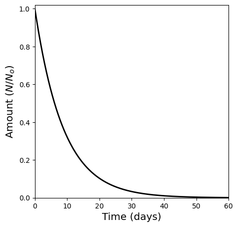
Radioactive decay is a statistical process, where the rate of decay must be proportional to the number of atoms remaining in the sample, or

\[ \frac{dN}{dt} = -\lambda N, \tag{1} \]

where $\lambda$ is the decay constant. Through separation of variables, Eqn. 1 can be integrated to give

\[ N(t) = N_o e^{-\lambda t}, \tag{2} \]

which depends on the original number of radioactive atoms $N_o$ and the half-life $\tau_{1/2}$ by

\[ \lambda = \frac{\ln\ 2}{\tau_{1/2}}. \]

import numpy as np
import matplotlib.pyplot as plt

fs = 'x-large'

tau_Ni = 6.1 #half-life of nickel-56 in days
lam_Ni = np.log(2)/tau_Ni
t = np.arange(0,60,0.1)

fig = plt.figure(figsize=(5,5))
ax = fig.add_subplot(111)

ax.plot(t,np.exp(-lam_Ni*t),'k-',lw=2)

ax.set_xlabel("Time (days)",fontsize=fs)
ax.set_ylabel("Amount ($N/N_o$)",fontsize=fs)
ax.set_ylim(0,1.02)
ax.set_xlim(0,60);

../_images/a3bc2f9be4c51cb37d42c5e41f9af4d04c51091eeec58d9d63e27b4ae96b9028.png

The deposition rate of the decay energy in to the supernova remnant must be proportional to $dN/dt$, the slope of the bolometric light curve is given by

\[ \frac{d\ \log_{10}\ L}{dt} = -0.434 \lambda, \tag{3} \]

or

\[ \frac{dM_{\rm bol}}{dt} = 1.086 \lambda. \tag{4} \]

Recall the extinction magnitude for the ISM. By measuring the slope of the light curve, we can determine $\lambda$ and verify the presence of large quantities of a specific radioactive isotope, like cobalt-56.

The most carefully studied supernova to date has been SN 1987A. As soon as it was discovered, astronomers realized that SN 1987A was unusual when compared with more distant Type II supernovae observations. It had a rather slow rise to the maximum light (taking 80 days), which peaked only at an absolute bolometric magnitude of $-15.5$, whereas a typical Type II peaks at $M_{\rm bol} = -18$.

https://github.com/saturnaxis/ModernAstro/blob/main/Chapter_15/Figure_12.jpg?raw=true? — Fig. 11.11 The bolometric light curve of 1987A through the first 1444 days after the explosion. The dashed lines show the contributions expected from the radioactive isotopes produced by the shock wave. (Carroll & Ostlie (2007); Figure adapted from Suntzeff et al. Ap. J. Lett., 384, L33 1992)#

Nickel-56 was produced by the shock and it totals $0.075\ M_\odot$ of material. The timescale for the decay energy to be radiated away is quite long and the decay energy produces a bump on the light curve near the maximum rather than forming a plateau. By the time the resulting cobalt-56 begins to decay, the decrease in luminosity of the remnant tracks closely with the cobalt-56. The next important radioactive isotope, cobalt-57, plays an important role in the development of the light curve of SN 1987A.

SN 1987A allowed astronomers to directly measure the X-ray and gamma-ray emission lines produced by radioactive decay for the first time. In particular, the 847 keV and 1238 keV lines of cobalt-56 were detected by a number of experiments, which confirmed the presence of the isotope.

11.3.4. The Subluminous Nature of SN 1987A#

The mystery of the subluminous nature of SN 1987a was solved after identifying its progenitor star, which was a spectral class B3 I blue supergiant, Sk -69 202. Since the progenitor was a BSG instead of a RSG (as is usually assumed), the star was more dense. Before the thermal energy produced by the shock could diffuse out and escape, it was converted into the mechanical energy required to lift the envelope of the star out of the deeper potential well of the blue supergiant. Measurements of ${\rm H\alpha}$ lines indicate that some of the outer hydrogen envelope was ejected at speeds of nearly $30,000\ {\rm km/s}$, or $0.1c$.

The available observations of Sk -69 202 tied with the theoretical evolutionary models suggest that the progenitor of SN 1987A had a mass of roughly $20\ M_\odot$ when it was on the main sequence and it lost a few solar masses ($\sim 1.4-1.6\ M_\odot$) before its iron core collapsed. Although it was apparently a RSG for $\sim 10^5-10^6\ {\rm yr}$, where it evolved to the BSG just 40,000 years before the explosion. Supporting this hypothesis is the observation that hydrogen was more abundant in the stellar envelope than helium, which suggests that the star had not suffered an extensive amount of mass loss.

11.3.5. Supernova Remnants#

There are now many examples of supernova remnants (SNR), such as the Crab Nebula that is located in Taurus. Nearly 1000 years since the SN 154 explosion, the Crab is still expanding a $\sim 1450\ {\rm km/s}$ and it has a luminosity of 80,000 $L_\odot$. Much of the emitted radiation is in the form of highly polarized synchrotron radiation, which indicates the presence of relativistic electrons that are spiraling around magnetic field lines. The ongoing source of the electrons and the continued high luminosity so long after the explosion were major puzzles until the discovery of a pulsar (i.e., a rapidly spinning neutron star) at the center of the Crab SNR. The Cygnus Loop nebula is another example of a SNR, where it is located 800 pc away and is 15,000 years old. The remnant shows shock fronts several AU wide as the debris from the supernova explosion encounters material in the ISM.

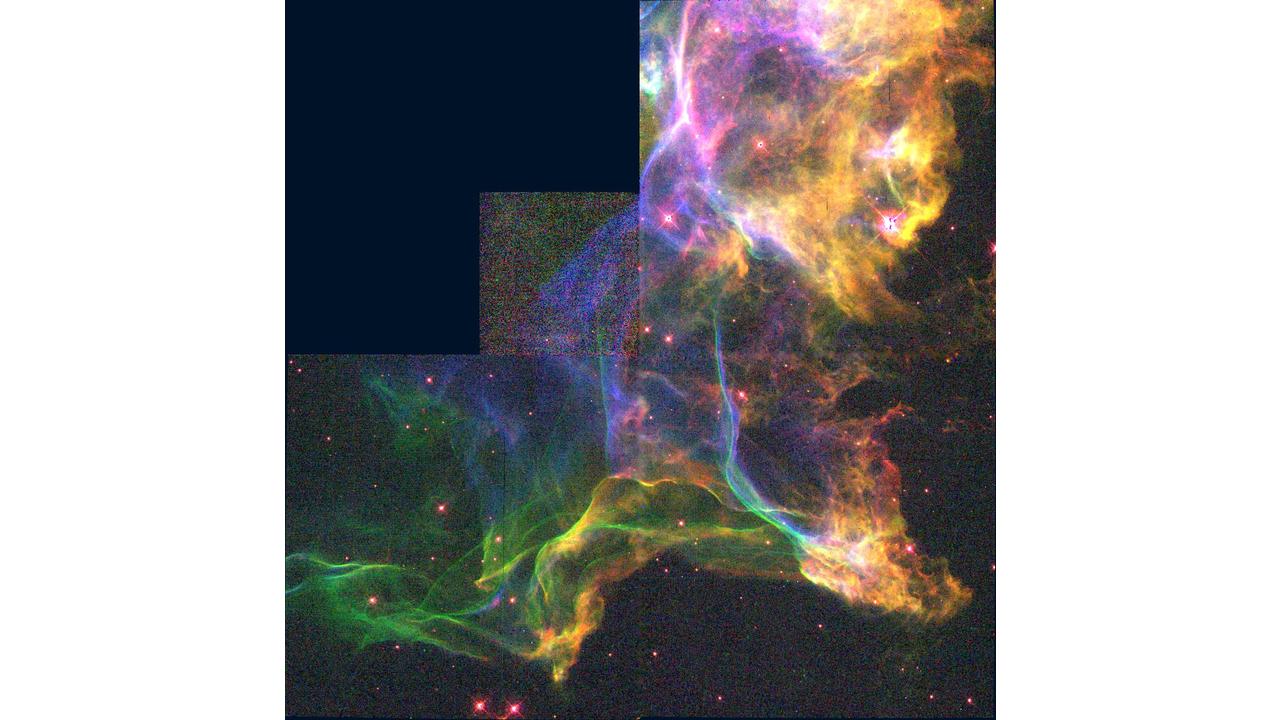
https://stsci-opo.org/STScI-01EVTAVVP6E5KE1VWK9FTDY9QV.jpg — Fig. 11.12 An HST WF/PC 2 image of a portion of the Cygnus Loop, 800 pc away. (Carroll & Ostlie (2007); Image Credit: J. Hester/Arizona State University and NASA)#

Mass loss prior to the supernova explosion of SN 1987A could not have been excessive, the progenitor did lose some mass that results in a very unusual structure around the expanding SNR. The Hubble Space Telescope has recorded three rings around SN 1987A, where the innermost ring measures 0.42 pc across and lies in a plane that contains the center of the SNR. It glows in the visible, which is a consequence of ${\rm O\ III}$ emission that is energized by the supernova’s radiation and appears elongated because it is inclined relative to our line of sight. The material making up the central ring was ejected by stellar winds 20,000 years before the explosion of SN 1987A.

https://apod.nasa.gov/apod/image/1202/sn1987a_hst_960.jpg — Fig. 11.13 Rings around SN 1987A detected by the Hubble Space Telescope in 2011. The diameter of the inner ring is 0.42 pc. (Carroll & Ostlie (2007); Image Credit: ESA/STScI, and NASA)#

The two larger rings lie in front of and behind the star (i.e., not in planes containing the central explosion). One explanation is that SK -69 202 had a nearby companion object (possibly a neutron star or black hole). As the companion source wobbles, narrow jets of radiation from the source would “paint” the rings in an hourglass-shaped bipolar distribution. In support of this hypothesis, researcher may have identified the source of these beams, which is about 0.1 pc from the center of the supernova explosion. Opponents of this model suggest that the explanation is too complicated, where it requires two sources of high-energy radiation: one to explain the central ring and another to explain larger ones. Alternatively the larger rings could be the product of a hot, fast stellar wind from the BSG progenitor overtaking the slower, cooler wind given off by the star when it was a RSG.

In the summer of 1990, fluctuating radio emission was detected from the supernova. Apparently the shock wave collided with clumps of material lost from SK -69 202 prior to the supernova explostion. The shock front from the expanding supernova remnant began to collide with the slower-moving stellar wind comprising the inner ring in 1996. Bright clumps in the inner ring developed over the next several years.

Mass loss prior to the supernova explosion of SN 1987A could not have been excessive, the progenitor did lose some mass that results in a very unusual structure around the expanding SNR. The Hubble Space Telescope has recorded three rings around SN 1987A, where the innermost ring measures 0.42 pc across and lies in a plane that contains the center of the SNR. It glows in the visible, which is a consequence of ${\rm O\ III}$ emission that is energized by the supernova’s radiation and appears elongated because it is inclined relative to our line of sight. The material making up the central ring was ejected by stellar winds 20,000 years before the explosion of SN 1987A.

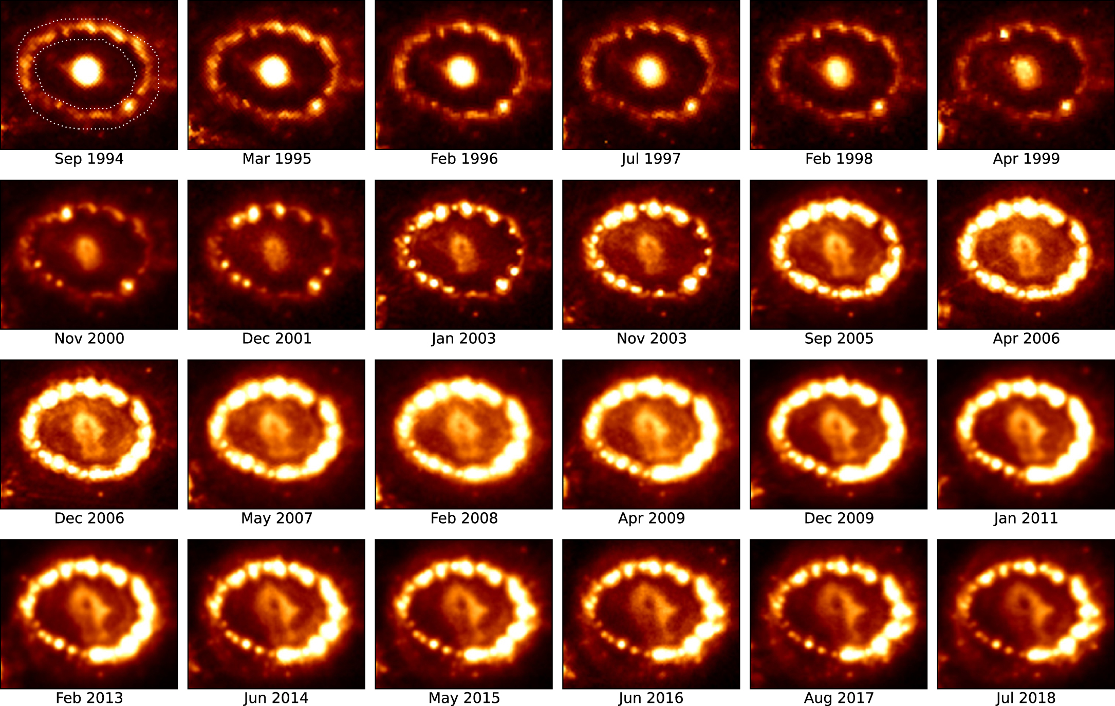
../_images/SN1987A_Rband.jpg — Fig. 11.14 Selection of images showing the evolution of SN 1987A in the R band. A mask which reduces the brightness of the ER by a factor of 14 has been applied to the images (shown by the dotted lines in the top left panel). Figure adapted from Larsson et al 2019 ApJ 886 147.#

11.3.6. The Detection of Neutrinos from SN 1987A#

One of the most exciting early observations of SN 1987A waw based on its nuetrinos, which represented the first time the neutrinos were detected from an astronomical source other than the Sun. The measurement confirmed the basic theory of core-collapse supernovae and provided near direct evidence for the formation of a neutron star out of the collapsed iron core.

The arrival of the neutrino burst wes recored over a duration of 12.5 seconds that was three hours before the arrival of the photons. Twelve events were recorded at Japan’s Kamiokande II Cerenkov detector and contemporaneously, eight events were detected by the IMB Cenrenkov detector near Fairport, OH. The neutrions began their trip ahead of the photons assuming the the exploding star became optically thin to neutrions before the shock wave reached the surface and the neutrionos traveled faster than the shock while still inside the star. Also the neutrinos must have been very near the speed of light to not be overtaken by the photons. There was not a significant dispersion in the neutrino energy, which suggests that the rest mass of the electron neutrions must be quite small. Based on data from SN 1987A, the electron neutrino mass was less than 16 eV, which is consistent with lab experiments that place the upper limit at 2.2 eV.

11.3.7. The Search for a Compact Remnant of SN 1987A#

Page et al. (2020) report a suspected detection of a compact in the remnant of SN 1987A. The purported detection comes from an IR excess due to the decay ${\rm ^{44}Ti}$, accretion luminosity from a neutron star or black hole, magnetospheric emission or a wind originating from the spin down of a pulsar, or to thermal emission from an embedded, cooling neutron star. The upper limit on the luminosity in the visible is less than $8\times 10^{26}\ {\rm W}$, which is equivalent to the optical energy output of an F6 main-sequence star. UV spectra lead to an upper limit of $L_{\rm UV} \leq 1.7 \times 10^{27}\ {\rm W}$, and Chandra has set an upper limit on the X-ray luminosity of $L_{\rm X} \leq 5.5 \times 10^{26}\ {\rm W}$ between 2-10 keV.

11.3.8. Chemical Abundance Ratios in the Universe#

A critical component in the evaluating the success of stellar evolution theory is the ability ot explain the observed elemental abundance ratios. The abundant element in the universe is hydrogen, followed by helium (reduced by a factor of 10). Current cosmological models produce all the hydrogen in the Big Bang that started the universe, which makes hydrogen primordial. Much of the present-day helium was also produced in the Big Bang, while the remainder of the elements are produced from fusion processes in stellar interiors.

https://github.com/saturnaxis/ModernAstro/blob/main/Chapter_15/Figure_16.jpg?raw=true? — Fig. 11.15 The relative abundances of elements in the Sun’s photosphere. All abundances are normalized relative to $10^{12}$ hydrogen atoms. (Carroll & Ostlie (2007); Data from Grevesse and Sauval, Space Sci. Rev., 85, 161, 1998.)#

Lithium, beryllium, and boron are less abundant than hydrogen and helium, but more so than what we would expect; they are depleted relative to the other elements. There are two reasons for this:

These elements are not (prominent) end products of nuclear reaction chains, and
They can be destroyed by collisions with protons.

For lithium this occurs at temperatures greater than $2.7 \times 10^6\ {\rm K}$, while beryllium requires a temperature greater than $3.5 \times 10^6\ {\rm K}$.

Surface convection is responsible for transporting the lithium, beryllium, and born from the surface to the interior. Comparing the elemental abundance of meteorites, we find that the relative abundances of beryllium are comparable, but the Sun’s surface abundance of lithium is reduced by a factor of about 100. This suggests that lithium has been destroyed in the Sun since its formation, but the beryllium has not been appreciably depleted.

Apparently the base of the solar convection zone extends deep enough to allow the lithium to burn, but not the beryllium. Combining stellar structure theory, the mixing-length theory of convection, and an analysis of solar oscillations, indicates that the base of the convection zone extends dow to only $2.3 \times 10^6\ {\rm K}$, which is not far enough to burn lithium adequately. Perhaps the momenta of the descending convective bubbles overshoot the bottom of the convective zone, causing lithium to be transported deeper than the standard models suggest. This disagreement is called the solar lithium problem and is an active area of research.

There are larger abundances for carbon, nitrogen, oxygen, neon, and so on because they are the end products of nuclear reaction chains at various stages of the star’s evolution. Core-collapse supernovae are responsible for significant quantities of oxygen, while Type Ia supernovae are responsible for most of the iron observed in the cosmos.

11.3.9. s-Process and r-Process Nucleosynthesis#

When nuclei with progressively higher values of $Z$ form via stellar nucleosynthesis, it becomes difficult for other charged particles (e.g., protons, alpha particles, etc.) to react with them. As $Z$ increases, so does the height of the Coulomb potential barrier. The same limitation does not exist for neutrons that collide with these nuclei. Nuclear reactions involving neutrons can occur even at relatively low temperatures. The reactions with neutrons have the form,

\[ {\rm ^A_ZX} + n \rightarrow {\rm ^{A+1}_ZX} + \gamma, \]

which result in more massive nuclei that can be stable or unstable against beta decay:

\[ {\rm ^{A+1}_ZX} \rightarrow {\rm ^{A+1}_{Z+1}X} + e^- + \overline{\nu}_e + \gamma. \]

If the beta-decay half-life:

is short compared to the timescale for neutron capture, then the capture reaction is a slow process, or a s-process reaction. Slow process reactions tend to yield stable nuclei, either directly or secondarily via beta decay.
is long compared with the timescale for neutron capture, then the capture is a rapid process, or a r-process reaction, which results in a neutron-rich nuclei.

These reactions appear at different times, where the s-process reactions occur during the normal phases of stellar evolution and the r-process reactions occur during a supernova (when a large flux of neutrinos exists). Neither process plays a significant role in energy production, but they do account for the abundance ratios of nuclei with $A>60$.

11.4. Homework#

Problem 1

During the Great Eruption of $\eta$ Car, the apparent visual magnitude reached a characteristic value of $m_V \sim 0$. Assume that the interstellar extinction to $\eta$ Car is 1.7 magnitudes and that the bolometric correction is essentially zero.

(a) Estimate the luminosity of $\eta$ Car during the Great Eruption.

(b) Determine the total amount of photon energy liberated during the twenty years of the Great Eruption.

(c) If $3\ M_\odot$ of material was ejected at a speed of $650\ {\rm km/s}$, how much energy went into the kinetic energy of the ejecta?

Problem 2

The angular extent of one of the lobes of $\eta$ Car is approximately $8.5^{\prime\prime}$. Assuming a constant expansion of the lobes of $650\ {\rm km/s}$, estimate how long it has been since the Great Eruption that produced the lobes. Is this likely to be an overestimate or an underestimate? Justify your answer.

Problem 3

Taking the distance to the Crab to be 2000 pc, and assuming that the absolute bolometric magnitude at maximum brightness was characteristic of a Type II supernova, estimate its peak apparent magnitude. Compare this to the maximum brightness of the planet Venus ($m\simeq -4$), which is sometimes visible in the daytime.

Problem 4

If the linear decline of a supernova light curve is powered by the radioactive decay of the ejecta, find the rate of decline (in ${\rm mag/day}$) produced by the decay of cobalt-56 into iron-56, with a half-life of 77.7 days.

Problem 5

The neutrino flux from SN 1987A was estimated to be $1.3 × 10^{14}\ {\rm m^{−2}}$ at the location of Earth. If the average energy per neutrino was approximately 4.2 MeV, estimate the amount of energy released via neutrinos during the supernova explosion.