7. The Interiors of Stars#
7.1. Hydrostatic Equilibrium#
7.1.1. Determining the Internal Structures of Stars#
Astronomers must generate computer models to deduce the detailed internal structure of stars, where these models mus be consistent with the known physical laws and agree with observable surface features. Much of the theoretical foundation was understood in the first half of the 20th Century, it wasn’t until the 1960s that computers were advanced enough to carry out all the calculations. Although computer modeling is a success, there are numerous questions that remain unanswered.
The theoretical study of stellar structure shows that stars are dynamic objects that typically change over very slow timescales (compared to us mortals), but some events can be very rapid and dramatic. Consider the observed energy output of the Sun, which is \(3.839 \times 10^{26}\) J of energy emitted per second. This energy output would be sufficient to melt a column of ice with a square mile area and 1 AU thick in only 0.3 seconds (assuming 100% absorption efficiency). Stars have a finite supply of energy, where they must eventually use up their fuel and die. Stellar evolution is the result of a constant fight against the relentless pull of gravity.
7.1.2. The Derivation of the Hydrostatic Equilibrium Equation#
The gravitational force is always attractive (as opposed to the electrostatic force that has opposite charges). Therefore, an opposing force (e.g., supplied by pressure) must exist in a star to avoid collapse. Just like the ocean, the pressure within a star varies with depth.
Consider a cylinder of mass \(dm\) whose base is located a distance \(r\) from the center of a spherical star.
The top and bottom of the cylinder each have an area \(A\) and the cylinder’s height is \(dr\).
Assume that the only forces acting on the cylinder are gravity and the force due to pressure, which is always normal (radially) to the top and bottom cylinder surface.
These forces also vary with the cylinder’s distance from the center of the star.
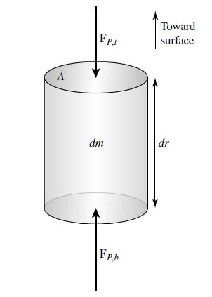
Fig. 7.1 In a static star the gravitational force on a mass element is exactly canceled by the outward force due to a pressure gradient in the star. Image credit: Carroll & Ostlie (2007).#
Using Newton’s second law \(\mathbf{F} = m\mathbf{a}\), we have the net force along the central axis of the cylinder:
where the gravitational force \(F_g\) and pressure force on the top of the cylinder \(F_{p,top}\) are directed inward (i.e., \(F<0\)), while the pressure force on the bottom \(F_{p,bot}\) of the cylinder is directed upward (i.e., \(F_{p,bot}>0\)). The pressure forces on the curved side of the cylinder will cancel due to symmetry and have been explicitly excluded from the expression.
The pressure force at the top and bottom of the cylinder are at different depths, and we can write a differential pressure force \(-dF_p = F_{p,bot}+F_{p,top}\). Then the equation from Newton’s second law can be rewritten as:
The gravitational force on a small mass \(dm\) located at a distance \(r\) from the center of a spherically symmetric mass is
which depends on the mass \(M_r\) inside the sphere of radius \(r\) (i.e., the interior mass). The pressure is defined as the amount of force per unit area (\(P\equiv F/A\)), where a pressure differential \(dP\) can be expressed as
Substituting Eqns. (7.2) & (7.3) into Eqn. (7.1) produces
The volume of a cylinder is product of the area \(A\) of the base with the height \(dr\), where the density of material enclosed \(\rho\) is the differential mass \(dm\) divided by the volume. The differential mass can be given as
and a substitution into Eqn. (7.4) becomes
Normalizing by the volume of the cylinder produces
which is the equation for the radial motion of the cylinder. For the hydrostatic case (i.e., \(\mathbf{a}=0\)), the radial motion equation becomes
where the local acceleration of gravity (at a radius \(r\)) is \(g\equiv GM_r/r^2\).
The condition of hydrostatic equilibrium represents a fundamental equation of stellar structure for spherically symmetric objects with negligible accelerations. A pressure gradient \(dP/dr\) must exist to counteract the gravitational force. It is not the pressure that supports a star, but the change in pressure with radius. The pressure must decrease with increasing radius so that the pressure is necessarily larger within the interior as compared to near the surface.
Exercise 7.1
What is an estimate of the pressure at the center of the Sun?
A very crude estimate can be made, if we assume that \(M_r = 1 M_\odot\), \(r=1 R_\odot\), \(\rho = \overline{\rho}_\odot = 1410 \:{\rm kg/m^3}\), and the surface pressure is exactly zero. Converting the differential equation for pressure into a difference equation yields
which depends on the central pressure \(P_c\). Substituting into Eqn. (7.7) provides an estimate of the central pressure as
GM_sun = 1.3271244e20 #GM_sun from astropy in m^3/s^2
R_sun = 6.955e8 #solar radius in m
rho_sun = 1410 #solar density in kg/m^3

P_c = GM_sun*rho_sun/R_sun
print("The estimated central pressure is %1.2e N/m^2" % P_c)
The estimated central pressure is 2.69e+14 N/m^2
A more rigorous calculation requires the integration of the hydrostatic equilibrium equation, where a functional form of the mass distribution (\(M_r\) and \(\rho\)) is needed. Unfortunately, explicit expression s are not available. A standard solar model gives a central pressure of \(2.34 \times 10^{16}\:{\rm N/m^2}\), which is \(\sim 100 \times\) larger than our crude estimate because there is an increased density near the center of the Sun. Using \(1.13 \times 10^5 \:{N/m^2}\) for Earth’s atmospheric pressure, the more realistic model of the Sun’s interior predicts a central pressure of \(2.3 \times 10^{11}\) atm.
7.1.3. The Equation of Mass Conservation#
Instead of using cylindrical symmetry, a relationship involving mass, radius, and density can be derived for spherical symmetry using Eqn. (7.5).
Consider a shell of mass \(dM_r\) and thickness \(dr\) located a distance \(r\) from the center of the shell.
Assume that the shell is sufficiently thin (i.e., \(dr \ll r\)).
The volume of the shell is approximately \(dV = A dr = 4\pi r^2\:dr\).
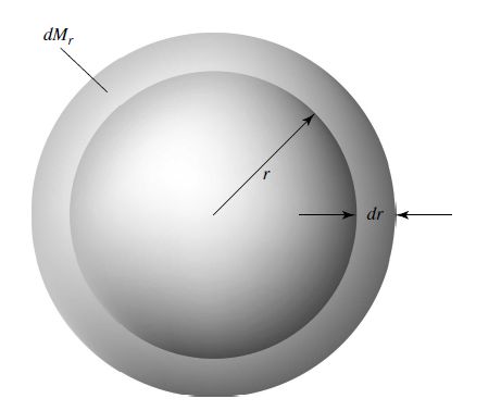
Fig. 7.2 A spherically symmetric shell of mass \(dM_r\) having a thickness \(dr\) and located a distance \(r\) from the center of the star. The local density of the shell is \(\rho\). Image credit: Carroll & Ostlie (2007).#
Using the relation for density \(\rho = M/V\), we arrive at the mass conservation equation,
which describes the mass distribution (i.e., changes in mass with radius) within a star.
7.2. Pressure Equation of State#
A gas has a several physical properties (mass, density, temperature, pressure, and volume) that describe how it currently exists (i.e., state). The state of a gas represents a macroscopic manifestation of the particle interactions and it is necessary to derive a pressure equation of state of the gas. One well-known example of a pressure equation of state is the ideal gas law, which is often expressed as
which relates the gas pressure \(P\), volume \(V\), and temperature \(T\) to the number of particles \(N\) (or \(n\)) and the Boltzmann constant \(k\) (or gas constant \(R\)). The ideal gas law is limited to specific environments, where in astrophysical problems it is necessary to have a pressure equation of state that is more general.
7.2.1. The Derivation of the Pressure Integral#
The pressure of a gas is the force per area exerted on the walls of its container due to collisions.
Consider a gas-containing cylinder of length \(\Delta x\) and ends with a cross-sectional area \(A\). The gas is composed of point particles, each of mass \(m\), that interact through perfectly elastic collisions.
The gas exerts a pressure on one of the ends of the container.
The impact of an individual particle on the container wall is described through a change in momentum.
Newton’s 2nd (\(\mathbf{F}=d\mathbf{p}/dt\)) and 3rd laws can be applied.
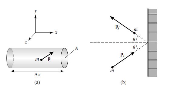
Fig. 7.3 (a) A cylinder of gas of length \(\Delta x\) and cross-sectional area \(A\). Assume that the gas contained in the cylinder is an ideal gas. (b) The collision of an individual point mass with one of the ends of the cylinder. For a perfectly elastic collision, the angle of reflection must equal the angle of incidence. Image credit: Carroll & Ostlie (2007).#
For a perfectly elastic collision, the angle of incidence equals the angle of reflection and we define a reference that is normal to the wall at the point of impact. Then the particle approaches the wall in the positive \(x\)-direction and rebounds along the negative \(x\)-direction. From Newton’s 3rd law, the impulse \(\mathbf{F}\Delta t\) delivered to the wall is just the negative of the change in momentum of the particle, or
using the \(x\)-component of the particle’s initial momentum \(p_x\). The average force exerted by the particle per time interval can be determined by the time interval between collision. The (shortest) time interval \(\Delta t\) is obtained when the particle traverses the length of the cylinder twice before returning for a second reflection, which is
so the average force exerted on the wall by a single particle over that time period is given by
where it is assumed that the force vector is normal to the surface. The numerator is proportional to \(v_x^2\) because \(p_x \propto v_x\). For a sufficiently large collection of particles in random motion, the likelihood of motion in each direction is the same (i.e., \(\overline{v}_x^2 = \overline{v}_y^2 = \overline{v}_z^2= v^2/3\)) so that \(v_x \approx v/\sqrt{3}\) and \(p_x v_x = pv/3\). The average force per particle having a momentum \(p\) is
However, it is usually the case that the particles have a range of momenta (i.e., range of incident angles). The number of particles with momenta between \(p\) and \(p + dp\) (similar to the Maxwell-Boltzmann distribution) is given by the expression \(N_p\:dp\) and the total number of particles in the container is
The contribution to the total force \(dF(p)\) by all the particles in a momentum range is
The sum of all the forces (i.e., integrating over all the possible momenta) exerted by particle collisions is
Normalizing the force exerted on the wall by the surface area \(A\) is the pressure on the surface. The volume of a cylinder is \(\Delta V = A \Delta x\) and defining \(n_p dp\) as the number fo particles per unit volume having a momenta within the range of \(p\) and \(p+dp\) can be written as
and we find the pressure exerted on the wall is
Equation (7.9) is sometimes called the pressure integral, which allows us to compute the pressure given some distribution function \(n_p dp\).
7.2.2. The Ideal Gas Law in Terms of the Mean Molecular Weight#
The pressure integral is valid for massive and massless particles (i.e., photons) traveling at any speed. For massive, nonrelativistic particles, we can use \(p=mv\) to write the pressure integral as
where \(n_v\:dv\) is the number of particles per unit volume having speeds between \(v\) and \(v+dv\) (i.e., \(n_v\:dv = n_p\:dp\)). In the case of an ideal gas, \(n_v\:dv\) is the Maxwell-Boltzmann velocity distribution,
where \(n\) is the total particle density for all velocities. Substituting into the pressure integral gives
using a table of definite integrals.
In astrophysical situations, the ideal gas law is more convenient in a different form because stars are measured in terms of the mass fractions (X, Y, and Z). Starting with the particle density \(n\), it can be related to the mass density of the gas as
which now depends on the average mass \(\overline{m}\) of a gas particle since the particles masses can vary. Then the ideal gas law becomes
The mean molecular weight is defined as
which scales the average mass by the mass of the hydrogen atom (essentially the mass of the proton). Then, the ideal gas law can be written in terms of the mean molecular weight \(\mu\) as
The mean molecular weight also depends on the ionization state of each molecular species, where the level of ionization enters because free electrons must be included in the average mass per particle \(\overline{m}\). This would require a detailed analysis using the Saha equation to calculate the relative numbers of ionization states, but it is easier when the gas is either completely neutral or completely ionized. For a completely neutral gas,
which depends on the mass and the total number of atoms (present in the gas) of type \(j\) denoted by \(m_j\) and \(N_j\), respectively. Normalizing each mass by the mass of a hydrogen atom \(m_H\) (\(A_j \equiv m_j/m_H\)) produces
and a similar expression can be derived for a completely ionized gas as
where the number of free electrons are accounted for using the \((1+z_j)\) factor. by inverting the expression for \(\overline{m}\), it is possible to derive an alternate equation for \(\mu\) in terms of the mass fractions. Recall that \(\overline{m} =\mu m_H\) and using Eqn. (7.13) gives,
and using the chain rule. The second term in the summation is simply the mass fraction \(X_j\) (i.e., mass of particles from \(j\) divided by the total mass of the gas). Through substitution,
Solving for \(1/\mu_n\), we have
For a neutral gas,
where the weighted average of all elements in the gas heavier than helium is \(\langle 1/A\rangle_n\) and for solar abundances this is approximately 1/15.5 or 0.0645.
The mean molecular weight for an completely ionized gas can be determined in a similar way, where it is only necessary to include the total number of particles contained in the sample because the number of free electrons matches the number of protons. For a completely ionized gas, Eqn 13 becomes
and including hydrogen and helium explicitly for Eqn. (7.16) produces
For elements much heavier than helium, \(1+z_j \simeq z_j\) and \(A_j \simeq 2z_j\), since the number of protons in the atom is much larger than 1 and that sufficiently massive atoms have approximately equal numbers of nucleons (i.e., protons and neutrons). Through substitution, we find
Using a composition representative of younger stars (X = 0.70, Y = 0.28, and Z = 0.02), the mean molecular weights are \(\mu_n = 1.30\) and \(\mu_i = 0.62\).
7.2.3. The Average Kinetic Energy per Particle#
Combining Eqn. (7.11) with the pressure integral (Eqn. (7.10)) produces the average kinetic energy per particle as
which can be rewritten to give
The left-hand side is just the integral average of \(v^2\) weighted by Maxwell-Boltzmann distribution function. Thus
or
Note
The factor of 3 arose from averaging particle velocities over the three degrees of freedom (or coordinate directions). Each degree of freedom contributes \(\frac{1}{2}kT\) to the average kinetic energy.
7.2.4. The Contribution Due to Radiation Pressure#
Photons possess momentum \((p=h\nu/c)\) and are capable of delivering an impulse to other particles during absorption or reflection. Electromagnetic radiation consists of a bundle of photons with a range of energies (and frequency \nu). The pressure integral (Eqn. (7.10)) is written in terms of momenta and thus, we can rederive the expression for radiation pressure using the pressure integral. Note that the pressure integral also depends on the velocity \(v\), but this dependence is removed if we substitute the speed of light for the velocity. We also assume an identity for the distribution function, \(n_p dp = n_\nu d\nu\) so that the pressure integral becomes
The expression \(n_\nu d\nu\) represents a distribution function that describes the number of photons with a frequency that lies between \(\nu\) and \(\nu + d\nu\). Multiplying by the energy for each photon results in \(h\nu n_\nu d\nu\), or the energy density \(u_\nu\) over the frequency integral, so that
Recall Eqn. (5.6) from the specific energy density section from Stellar Atmospheres provides the integral of the energy density as
and the radiation pressure is
The photon pressure can actually exceed the gas pressure by a significant amount and even surpass the gravitational force (e.g., variable stars). The full pressure of the stellar interior can written by combining the contributions from an ideal gas (Eqn. (7.12)) and the radiation pressure (Eqn. (7.20)) as
Exercise 7.2
What is the central temperature of the Sun (neglecting the radiation pressure)?
From hydrostatic equilibrium, we estimated the central pressure \(P_c\). Thus, we can rewrite the radiation pressure equation from the ideal gas law (Eqn. (7.12)) as
Using \(\rho = \overline{\rho}_\odot = 1410 \:{\rm kg/m^3}\), \(\mu_i =0.62\) (assuming complete ionization of \(H\)), and \(P_c = 2.69 \times 10^{14}\: {\rm N/m^2}\), we find that
which is in reasonable agreement with more detailed calculations. One standard solar model shows the radiation pressure is only 0.065% of the gas pressure, which justifies our simplification in ignoring it.
from scipy.constants import k

m_H = 1.6735575e-27 #mass of hydrogen
rho_sun = 1410. #average density of the Sun in kg/m^3
P_c = 2.69e14 #Central pressure estimated in previous example in N/m^2
mu_i = 0.62 #mass ratio assuming complete ionization of H

T_c = (mu_i*m_H)/(rho_sun*k)*P_c

print("The estimated central temperature of the Sun is %1.2e K." % T_c)
The estimated central temperature of the Sun is 1.43e+07 K.
7.3. Stellar Energy Sources#
7.3.1. Gravitation and the Kelvin-Helmholtz Timescale#
In the late 1800s, many scientists were contemplating the energy source of the Sun. One likely stellar energy source is gravitational potential energy, which is given by
using the Universal Gravitational constant \(G\), masses of two particles (\(M\) and \(m\)), and the distance between them \(r\). As \(r\) decreases, the gravitational potential energy becomes more negative, implying that the energy must have been converted to other forms (e.g., kinetic energy). If a body can decrease its size, then the gravitational potential energy can be converted into heat and then radiate into space. The star could shine for a significant period of time through this mechanism. However, the virial theorem state that the total energy \(E\) for a system in equilibrium is 1/2 of a system’s potential energy \(U\). Therefore, only half of the system’s potential energy is available to be radiated away and the remaining potential energy supplies the thermal energy that heats the star.
Note
Radiation derived from gravitational contraction is a source of energy for Jupiter-mass planets and brown dwarfs.
The contribution of every pair of particles to the potential energy can be calculated starting with the gravitational force and some assumptions.
Assume a point mass \(dm_i\) exists outside a spherically symmetric mass \(M_r\).
The gravitational force is
where the force is directed toward the center of the sphere. Due to the symmetry, we can replace the massive sphere with an equivalent mass located at its center, which is separated by a distance \(r\) from the point mass \(dm_i\). Then the gravitational potential energy is
Instead of using a point mass \(dm_i\), we can assume that a collection of smaller point masses distributed uniformly within a shell of thickness dr with a mass \(dm\) (i.e., \(\displaystyle dm = \sum_i dm_i\)). These quantities are related by
given the mass density \(\rho\) of the shell and its volume, \(4\pi r^2\:dr\). The equation for differential gravitational potential energy becomes
by direct substitution and the total gravitational potential energy is
where the integral is from the center to the radius \(R\) of the star. More exact calculations of \(U_g\) requires knowledge of the radial mass distribution (\(\rho\) and \(M_r\)) within a body. However, we can use the average mass density of the Sun \(\overline{\rho}_\odot\) to produce an estimate. The average density is the total mass contained in a volume, or
where solving for \(M_r\) becomes
Substituting into Eqn. (7.22), the total gravitational energy becomes
Back-substituting \(\overline{\rho}\) to get an expression in terms of the total mass \(M\) and radius \(R\) of the star produces
Applying the virial theorem shows that the total mechanical potential energy is
Exercise 7.3
If the Sun had an initial radius \(R_i\) and was originally much larger than it is today (\(R_i \gg R_\odot\)), how much energy would have been released due to its gravitational collapse?
The energy released \(\Delta E\) is simply the difference in energy from the initial state \(E_i\) to the current state \(E_f\), or \(\Delta E = -(E_f - E_i)\). The virial theorem shows that the energy of a very large object (\(R_i \gg R_\odot\)) is very small because \(E \propto 1/R\). Therefore, \(E_i \approx 0\) and the change in energy simplifies to
from scipy.constants import G

M_sun = 1.989e30 #mass of the Sun in kg
R_sun = 6.955e8 #radius of the Sun in m
L_sun = 3.828e26 #luminosity of the Sun in W

delta_E = 0.3*(G*M_sun**2/R_sun)
t_KH = (delta_E/L_sun)/3600./24./365.25 #timescale in s-->yr

print("The energy released by the gravitational collapse of the Sun is %1.2e J." % delta_E)
print("The timescale for releasing this much energy is %1.1e yr" % t_KH)
The energy released by the gravitational collapse of the Sun is 1.14e+41 J.
The timescale for releasing this much energy is 9.4e+06 yr
Assuming the luminosity of the Sun has been roughly constant throughout its lifetime, it could emit energy at that rate for approximately
A solar luminosity is \(3.828 \times 10^{26}\) W, where \(t_{KH} \sim 10^7\) yr and is known as the Kelvin-Helmholtz timescale. The Kelvin-Helmholtz timescale was developed by Lord Kelvin and Hermann Ludwig Ferdinand von Helmholtz (in the late 1800s) to explain the Sun’s energy source, but geological (relative) dating techniques at the time was producing rock ages that were at least an order of magnitude older. Today, we have radioactive dating of Earth rocks, Moon rocks, and primitive meteorites that are more than ~4.5 Gyr old. Therefore, gravitational potential energy alone cannot account for the Sun’s luminosity through its entire lifetime.
Note
Another possible energy source involves chemical processes, but chemical reactions are based on the orbital electrons in atoms. The amount of energy available to be released per atom is no more than 10 eV. Given the number of atoms present in a star, the amount of chemical energy available is far to low to account for the Sun’s luminosity over a reasonable period of time.
7.3.2. The Nuclear Timescale#
Since electron orbits contributes less than 10 eV, nuclear processes involve energies in the millions of electron volts (MeV) range. The nucleus of a particular element is specified by the number of positively charged protons \(Z\) (not to be confused the metal mass fraction). A neutrally charged atom would contain an equal number of orbital electrons. Isotopes of a given element are identified by the number of (neutrally charged) neutrons \(N\) within the nucleus. Collectively, protons and neutrons are referred to as nucleons, where the number of nucleons is represented by the mass number \(A = Z + N\). The mass number is a good heuristic to estimate the mass of an isotope because protons and neutrons have similar masses, where the mass of electrons is much smaller than either protons or neutrons.
The respective masses of the proton, neutron and electron are
\(m_p = 1.67262158 \times 10^{-27}\:{\rm kg} = 1.00727646688 \: {\rm u} = 938.27208816 \: {\rm MeV},\)
\(m_n = 1.67492716 \times 10^{-27}\:{\rm kg} = 1.00866491578 \: {\rm u} = 939.56542052 \: {\rm MeV},\) and
\(m_e = 9.10938188 \times 10^{-31}\:{\rm kg} = 0.0005485799110 \: {\rm u} = 0.51099895000 \: {\rm MeV}.\)
The atomic mass unit \(u\) is defines as exactly 1/12 the mass of the Carbon-12, or \(1\:{\rm u} = 1.66053873 \times 10^{-27}\:{\rm kg}\). The rest mass energies are derived using Einstein’s \(E=mc^2\), where \(1\:{\rm u} = 931.494013\:{\rm MeV/c^2}\). The simplest isotope of hydrogen is composed of a single proton and electron with a mass of \(m_H = 1.00782503214\:{\rm u}\). This mass is slightly less than the combined mass of a proton and electron at rest (\(m_p + m_e\)) because some mass must be given up as binding energy to keep the atom together. For a hydrogen atom in its ground state, the exact mass difference is 13.6 eV, which is just the ionization potential.
Note
Mass-energy units are \({\rm MeV/c^2}\) as follows from \(E=mc^2\), but it is customary to leave off the \({\rm /c^2}\). When using mass-energy units in your calculations, be sure to multiply by \(c^2\) to get units of energy.
Similarly energy is also released for a loss in mass when nucleons combine to form atomic nuclei. A helium nucleus is composed of two protons and two neutrons, which can be formed by a series of nuclear reactions involving four protons (hydrogen nuclei) otherwise known as fusion reactions since lighter particles are fused together to form a heavier particle. The total mass of the four hydrogen atoms (protons and electrons) is 4.03130013 u, where as the mass of one helium atom is 4.002603 u. The mass difference between these two quantities is 0.028697 u, or 0.7%. The total amount of energy released in forming a helium nucleus is the binding energy and is equivalent to the mass difference but in energy units (26.731 MeV). The helium nucleus requires 26.731 MeV to free the nucleons into the constituent protons and neutrons.
Exercise 7.4
Is nuclear energy sufficient to power the Sun during its lifetime? (Assume that the Sun started with 100% hydrogen and only converts 10% of that into helium.)
The mass available is 10% of the Sun’s mass converted into energy (\(M_\odot{\rm c^2}\)). To form a helium nucleus, only 0.7% of the energy is released.
This gives a nuclear timescale of approximately
which is more than enough time to account for the ages of rocks on Earth and the Moon.
from scipy.constants import c

m_sun = 1.989e30 #mass of Sun in kg
E_nuc = 0.007*0.1*m_sun*c**2
t_nuc = (E_nuc/L_sun)/3600./24./365.25

print("The amount of nuclear energy available is %1.2e J." % E_nuc)
print("The nuclear timescale is %1.2e yr." % t_nuc)
The amount of nuclear energy available is 1.25e+44 J.
The nuclear timescale is 1.04e+10 yr.
7.3.3. Quantum Mechanical Tunneling#
Inside of stars, nuclear reactions occur through collisions, which form new nuclei in the process. However, all nuclei are positively charged and a Coulomb potential energy barrier must be overcome so that fusion can occur. In a proton-proton interaction, there are two main regimes:
Coulomb repulsion dominates which forces the nuclei apart
and
a potential well governed by the strong nuclear force that binds the nucleus together,
where the transition between regions occurs when the nuclei are \(\sim 10^{-15}\) m, or 1 fm, apart. While the Coulomb force is repulsive, the strong nuclear force is an attractive force that acts on incredibly short distances.
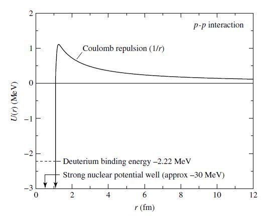
Fig. 7.4 The potential energy curve characteristic of nuclear reactions. Image credit: Carroll & Ostlie (2007).#
One source of energy that nuclei could use to overcome the Coulomb barrier is provided by the thermal energy of the gas (i.e., momentum carries the particles to mergers). In this scenario, we assume that all nuclei are moving nonrelativistically and then the required temperature can be estimated. All of the particles in the gas are in random motion and it is then appropriate to refer to the relative velocity \(v\) between nuclei and their reduced mass \(\mu_m\). Note that this is not the mean molecular weight \(\mu\). To overcome the Coulomb repulsion, the initial kinetic energy of the reduced mass must exceed the potential energy of the barrier (i.e., the classical “turn-around point”). Using Eqn. (7.18), we have
which depends on the temperature \(T_{classical}\) required to overcome the barrier, the numbers of protons in each nucleus (\(Z_1\) and \(Z_2\)), and their separation \(r\). Assuming a typical nucleus radius is 1 fm, the temperature needed to overcome the Coulomb potential energy barrier is approximately,
for two protons.
from scipy.constants import k, epsilon_0, e, pi

Z_1 = 1 #number of protons in particle 1
Z_2 = 1 #number of protons in particle 2
r = 1e-15 #radius of nucleus in fm
T_classical = (Z_1*Z_2*e**2)/(6*pi*epsilon_0*k*r)
print("The classical temperature to overcome Coulomb repulsion is %1.2e K" % T_classical)
The classical temperature to overcome Coulomb repulsion is 1.11e+10 K
The central temperature of the Sun is only 15.7 million K (or \(1.57 \times 10^7\:{\rm K}\)), which is about \(1000 \times\) lower. Even accounting for the velocity dispersion expected through the Maxwell-Boltzmann distribution indicates that classical physics is unable to explain how a sufficient number of particles can overcome the Coulomb barrier to produce the Sun’s luminosity.
Quantum mechanics’ inherent uncertainty tells us that we can’t know both the position and momentum of a particle with unlimited accuracy (i.e., \(\Delta x \Delta p \ge \hbar/2\)). In other words, the uncertainty in position of one proton is so large that in can still find itself within the potential well defined by the strong force. This quantum mechanical tunneling effect has no classical counterpart. A large ratio of the potential energy to the kinetic energy makes tunneling less likely.
As a crude estimate of the tunneling effect, assume that a proton must be within approximately 1 de Broglie wavelength (\(\lambda = h/p\)) of its target to tunnel through the Coulomb barrier. The reduced mass kinetic energy can be rewritten as
and the distance of close approach (\(r=\lambda=h/p\)) gives
Solving for \(\lambda\) produces
which can be substituted into Eqn. (7.27) to get
for the temperature required for a reaction to occur. For two protons, \(\mu_m = m_p/2\) and \(Z_1 = Z_2 = 1\). Then, we find that \(T_{quantum} \sim 10^7\:{\rm K}\), which is consistent with the estimated central temperature of the Sun.
from scipy.constants import k, epsilon_0, e, pi, m_p, h

Z_1 = 1 #number of protons in particle 1
Z_2 = 1 #number of protons in particle 2
mu_m = m_p/2. #reduced mass of two protons
T_quantum = (mu_m*(Z_1*Z_2*e**2)**2)/(12*(pi*epsilon_0*h)**2*k)
print("The quantum temperature to overcome Coulomb repulsion is %1.2e K" % T_quantum)
The quantum temperature to overcome Coulomb repulsion is 9.79e+06 K
7.3.4. Nuclear Reaction Rates and the Gamow Peak#
We need to know the nuclear reaction rates to develop a stellar model. Not all particles in a gas of temperature \(T\) will have sufficient kinetic energy and the necessary wavelength to tunnel through the Coulomb barrier. The reaction rate per energy interval must be described in terms of the number density of particles having energies within a particular range combined with the probability for successive quantum tunneling. The total nuclear reaction rate is then integrated over all possible energies.
Consider the number density of nuclei within a specified energy interval \(n_E dE\). The Maxwell-Boltzmann distribution relates the number density of particles with a velocity \(v\) within an interval \(dv\) to the temperature of a gas. The nonrelativistic kinetic energy describes the total energy of the particles (\(K = E = \mu_m v^2/2\)) when the potential energy is negligible. We can then write the Maxwell-Boltzmann distribution in terms of the number of particles with kinetic energies between \(E\) and \(E+dE\) as
Equation (7.29) describes the energy density in the range \(dE\), but not the probability that particles will actually interact. The interaction probability depends on the cross-section. The cross-section as a function of energy \(\sigma(E)\) is defined as
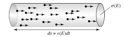
Fig. 7.5 The number of reactions per unit time between particles of type \(i\) and a target \(x\) of cross section \(\sigma(E)\) may be thought of in terms of the number of particles in a cylinder of cross-sectional area \(\sigma(E)\) and length \(ds = v(E) dt\) that will reach the target in a time interval \(dt\). Image credit: Carroll & Ostlie (2007).#
Although \(\sigma(E)\) is strictly a probability, it can be interpreted as roughly the cross-sectional area of the target particle, where any incoming particle that strikes within the cross-sectional area will result in a nuclear reaction. Consider the number of particles that will hit a target of cross-sectional area \(\sigma(E)\). Let \(x\) represent a target particle and \(i\) denote an incident particle. Then the number of reactions \(dN_E\) is the number of particles that can strike \(x\) in a time interval \(dt\) with a velocity \(v(E) = \sqrt{2E/\mu_m}\). The number of incident particles are those contained within a cylinder of volume \(\sigma(E)v{E}dt\), or
The number of incident particles per unit volume with the appropriate velocity (or kinetic energy) is a fraction of the total number of particles within the sample,
where Eqn. (7.29) defines \(n_E dE\). The number of reactions per target nucleus per time interval \(dt\) within a range of energy is
If there are \(n_x\) targets per unit volume, the total number of reactions per unit volume per unit time, integrated over all possible energies is
Now that we have a form for the reaction rate, we need to know \(\sigma(E)\) and unfortunately, it changes rapidly with energy which makes it complicated. Stellar thermal energies are quite low compared to lab measurements and significant extrapolation is usually required. The process for determining \(\sigma(E)\) can be improved if the terms most strongly dependent on energy are factored out first. We have suggested that:
the cross section can be roughly interpreted as a physical area,
and
the size of a nucleus is approximately one de Broglie wavelength in radius (\(r\sim\lambda\)).
Combining these ideas,
where in the nonrelativistic limit \(p^2 \propto E\). The ability to tunnel through the Coulomb barrier is related to the ratio of the potential barrier height and the initial kinetic energy of the incoming nucleus. If the barrier height \(U_c\) is small (\(U_c\sim 0\)), then the tunneling probability goes to 1 (100% probable). As the barrier height increases, the probability of tunneling must decrease and asymptotically approach zero as the potential barrier height goes to infinity. This is described by an exponential and we have
where the \(2\pi^2\) arises from the quantum mechanical treatment of the problem. The ratio of the barrier height to the kinetic energy is
using \(\lambda = h/p\) and \(p = \mu_m v\). After some additional manipulation, we find that
where
The factor \(b\) depends on the masses and electric charges of the two nuclei involved in the interaction. Combining our estimate of \(\sigma(E)\) and defining \(S(E)\) as some (we hope) slowly varying function of energy, we may now express the cross section as
Then the reaction rate integral (Eqn. (7.30)) becomes
Equation (7.34) includes the term \(e^{-E/(kT)}\) to represent the high energy wing of the Maxwell-Boltzmann distribution and the term \(e^{-b/\sqrt{E}}\) to represent the tunneling probability. The product of these factors produces a strongly peaked curve, known as the Gamow peak. The top to the curve occurs at the energy
The greatest contribution to the reaction rate integral comes in a fairly narrow energy band that depends on the temperature of the gas along with the charges and masses of the reaction constituents.
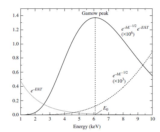
Fig. 7.6 The likelihood that a nuclear reaction will occur is a function of the kinetic energy of the collision. Image credit: Carroll & Ostlie (2007).#
7.3.5. The Luminosity Gradient Equation#
To determine the luminosity of a star, we must now include all the potential contributions to energy production. The contribution to the luminosity due to an infinitesimal mass \(dm\) is
which includes the total energy release per second per kilogram \(\epsilon\) by all nuclear reactions and gravity, \(\epsilon = \epsilon_{nuclear} + \epsilon_{gravity}\). The contribution from gravity \(\epsilon_{gravity}\) could be negative, if the star is expanding instead of contracting. For a spherically symmetric star, the mass of a thin shell of thickness \(dr\) is just
which can be directly substituted to get
Similar to \(M_r\), the luminosity generated by the mass interior to a radius \(r\) is \(L_r\). Equation (7.36) is a fundamental stellar structure equation.
7.3.6. Stellar Nucleosynthesis and Conservation Laws#
The process of creating more complex atoms is called nucleosynthesis. We started investigating this process when discussing the nuclear timescale, which depended upon a process that converted 4 hydrogen atoms into helium. It is unlikely that this would occur through a 4-body collision (i.e., all four atoms hitting simultaneously). The process occurs through a chain of smaller reactions, each involving the more probably two-body interactions.
The chain of nuclear reactions cannot happen in a completely arbitrary way, where a series of particle conservation laws must be obeyed. During every reaction it is necessary to conserve: electric charge, the number of nucleons (e.g., protons and neutrons), and the number of leptons (e.g., electrons, positrons, neutrinos, and antineutrinos).
Antimatter is extremely rare in comparison with normal matter, but it plays a crucial role in subatomic physics to ensure the conservation laws are obeyed. Antimatter particles are identical to their matter counter parts, but have a singular, opposite attribute (e.g., charge). Antimatter also has an attribute where it completely annihilates upon collision with normal matter, where the excess energy is released in the form of energetic photons. For instance,
which describes the interaction between an electron \(e^-\) and a positron \(e^+\) to produce 2 photons \(\gamma\). Note that the two photons are required to conserve both momentum and energy simultaneously.
Neutrinos \(\nu\) and antineutrinos \(\overline{\nu}\) are electrically neutral particles and have a very small (but non-zero) mass (\(m_\nu \le 0.8\:{\rm eV/c^2}\)). A neutrino has a very small interaction cross-section (\(\sigma_\nu \sim 10^{-48}\:{\rm m^2}\)) with other matter, which makes them very difficult to detect. Such a small cross-section, even at the high densities of the stellar interior, implies that a neutrino’s mean free path is on the order of \(10^{18}\:{\rm m}\sim 10\:{\rm pc}\) (or nearly \(10^9 R_\odot\)). After their creation in a nuclear reaction, neutrinos almost always escape from the star, with the exception of a supernova explosion.
Note
A low mass particle was proposed by Wolfgang Pauli in 1930 to conserve certain reaction processes including energy and momentum. In 1934, Enrico Fermi dubbed these particles neutrinos, or little neutral ones.
Positrons and protons have an equal amount of charge, where the lepton (positron) will contribute to the charge and lepton number conservation requirement. Specifically the total matter leptons minus the total number of antimatter leptons must remain constant. To assist in the counting of the number of nucleons and the total electric charge, nuclei will be represented by
where the chemical symbol of the element (\({\rm H}\) for hydrogen, \({\rm He}\) for helium, etc.) is used in place of \({\rm X}\). The number of protons \(Z\) and the mass number \(A\) are also used.
7.3.7. The Proton-Proton Chain#
Through conservation laws, one chain reaction can convert hydrogen into helium and is known as the proton-proton chain (PPI). It involves a reaction sequence that produces deuterium \((^2_1{\rm H})\) and helium-3 \((^3_2{\rm He})\) as intermediate products before successfully producing stable helium-4 \((^4_2{\rm He}\)). The entire PP I chain is
where \({^1_1{\rm H}}\) represents a proton due to the high temperatures (ionizing) required for the reaction to occur. Each step in the PP I chain has its own reaction rate, since different Coulomb barriers and cross-sections are involved. The initial step is the slowest because it involves the decay of a proton into a neutron via \(p^+ \rightarrow n + e^+ \nu_e\) to make the deuterium (\(^2_1{\rm H}\)).
Note
There are four forces of nature: 1) the gravitational force that affects all particles with mass-energy, 2) the electromagnetic force that affects charged particles, 3) the strong force that binds nuclei together, and 4) the weak force of radioactive beta (electron/positron) decay. The decay of a proton is an example of the weak force.
The production of helium-3 nuclei from the PP I chain provides the possibility of their interaction directly with the helium-4 nuclei to produce the PP II chain. In an environment like the Sun, helium-3 interacts with another helium-3 for 69% of the time and the remainder of the time (31%) the PP II chain occurs:
which introduces beryllium-7 \((^7_4{\rm Be})\) and lithium-7 \((^7_3{\rm Li})\) as intermediate products. Another branch, the PP III chain, is possible through the capture of an electron by the beryllium-7 \((^7_4{\rm Be})\) in the PP II chain that competes with the capture of a proton (only 0.3% of the time) to produce boron-8 \((^8_5{\rm B})\). The PP III chain is:
which produces beryllium-8 \((^8_4{\rm Be})\) that decays into 2 helium-4 nuclei. Examining the nuclear energy generation rate shows that the pp chain has a temperature dependence of \(T^4\) near \(1.5 \times 10^7\:{\rm K}\).
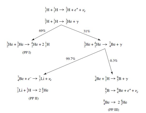
Fig. 7.7 The three branches of the pp chain, along with the branching ratios appropriate for conditions in the core of the Sun. Image credit: Carroll & Ostlie (2007).#
7.3.8. The CNO Cycle#
A second, independent cycle exists for the production of helium-4 from hydrogen, but it involves heavier nuclei: carbon, nitrogen, and oxygen. The CNO cycle uses the heavy nuclei as catalysts that are generated and consumed during the process. Like the pp chain, the CNO cycle has competing branches. The first branch (CNO I) produces carbon-12 and helium-4:
which occurs most of the time (99.96%). It also produces several intermediate isotopes of carbon, nitrogen, and oxygen that are consumed by the process. The second branch (CNO II) occurs only 0.04% of the time and arises when the final reaction of the CNO I chain produces oxygen-16 and a photon rather than carbon-12 and helium-4. The CNO II chain is:
which produces and consumes fluorine-17 \((^{17}_9{\rm F})\). A similar analysis of the nuclear energy generation rate shows that the CNO cycle has a much higher temperature dependence of \(T^{19.9}\) near \(1.5 \times 10^7\:{\rm K}\). This implies that low-mass stars with lower central temperatures are dominated by the pp chains during their hydrogen burning evolution, whereas high-mass stars can generate the central temperatures necessary to convert hydrogen into helium through the CNO cycle.
A consequence of both the pp chain and the CNO cycle is the mean molecular weight \(\mu\) of the gas increases. If the temperature and the gas density remain constant, then the ideal gas laws predicts that the central pressure will decrease and the star will begin to collapse. The collapse actually raises the temperature and gas density to compensate for the increase in \(\mu\). When the temperature and gas density are sufficiently high, then the helium nuclei can overcome their Coulomb repulsion and begin to burn (i.e., convert into heavier nuclei).
Note
The CNO cycle was proposed by Hans Bethe (1906-2005) in 1938, just six years after the discovery of the neutron.
7.3.9. The Triple Alpha Process of Helium Burning#
For sufficiently high temperatures, helium (i.e., an \(\alpha\) particle) can be converted into carbon through the triple alpha process. The triple alpha process is:
In the triple alpha process, an unstable beryllium-8 is produced by the fusion of two alpha particles and will rapidly decay back into two separate helium nuclei if not immediately struck by another alpha particle. The reaction rate depends on \((\rho Y)^3\) and the nuclear energy generation rate has a much higher temperature dependence \((T^{41})\). With such a strong dependence on temperature, even a small increase will produce a large increase in the amount of energy generated per second.
7.3.10. Carbon and Oxygen Burning#
Beyond helium burning, other competing processes can be at work due to the availability of carbon from the triple alpha process. It is now possible for carbon to capture alpha particles to become oxygen and some of those oxygen can capture alpha particles to become neon through
The ever higher Coulomb barrier of heavy nuclei limits this process to only very high temperatures. If a star is sufficiently massive, still higher central temperatures can be obtained. The star can achieve carbon burning reactions near \(6 \times 10^8\:{\rm K}\),
and oxygen burning reactions near \(10^9\:{\rm K}\),
In some reactions energy is absorbed rather than released (i.e., endothermic), where the other reactions energy is released (i.e., exothermic). In endothermic reactions, the product nucleus actually possesses more energy per nucleon than did the nuclei from which it formed. In general, endothermic reactions are much less likely to occur under normal conditions in stellar interiors.
7.3.11. The Binding Energy per Nucleon#
The energy release in nuclear reactions depends on the binding energy per nucleon \(E_b/A\), where
and depends on then number of protons \(Z\), the mass number \(A\) (to determine the number of neutrons), and the mass of the nucleus \(m_{nucleus}\). The binding energy per nucleon \(E_b/A\) increases rapidly for lighter elements (\(A\lesssim 24\)) and then begins to decrease at \(A=56\). Unusually stable nuclei are helium-4, oxygen-16, and hydrogen-1, which are unsurprisingly the most abundant nuclei in the universe. The stability arises from the shell structure of the nucleus and these nuclei are called magic nuclei.
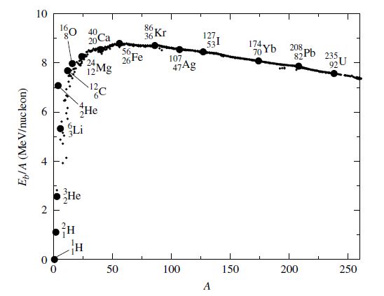
Fig. 7.8 The binding energy per nucleon \(E_b/A\) as a function of mass number \(A\). Image credit: Carroll & Ostlie (2007).#
Note
Shortly after the Big Bang, the early universe was composed primarily of hydrogen and helium, with no heavy elements. The study of nucleosynthesis strongly suggests that the heavy nuclei were generated in the interiors of stars. Thus, we are all “star dust” and have risen from the ashes of previous generations of stars.
The most stable of all nuclei occurs for \({^{56}_{26}Fe}\), which corresponds the peak in the binding energy per nucleon. Stellar interiors build up nuclei starting from lighter elements and approach the iron peak, where each successive fusion reaction results in the liberation of energy. Past the peak, it takes more energy to hold the nuclei together and fission reactions become more likely. Stars are iron making machines, but they require sufficient energy to overcome the Coulomb barrier.
7.4. Energy Transport and Thermodynamics#
7.4.1. Three Energy Transport Mechanisms#
In stellar interiors, energy is transported through radiation, convection, and conduction.
Radiation allows the energy produced by nuclear reactions and gravitation to be carried to the surface via photons. The photons are absorbed and re-emitted in nearly random directions as the encounter matter, where the opacity must play an important role.
Convection can be more efficient in some parts of the star with hot, buoyant mass elements carrying excess energy outward while cool elements fall inward (i.e., an energy escalator).
Conduction transports heat via collisions between particles, which is the least efficient method for stellar environments. As a result, it is generally insignificant throughout a majority of the stellar lifetime.
7.4.2. The Radiative Temperature Gradient#
For radiation transport, we need a description of how the radiation varies with the distance from the center \(r\). The radiation pressure gradient is given by,
and depends on the outward radiative flux \(F_{rad}\). From Eqn. (7.20) (see Sect. 7.2.4), the radiation pressure gradient may be expressed as
which depends on the radiation constant \(a=4\sigma/c\). Solving for \(dT/dr\) in terms of \(F_{rad}\), produces
Using the basic definition for radiative flux given the local radiative luminosity \(L_r\) at a radius \(r\),
and the temperature gradient for radiative transport becomes
As either flux or opacity increases, the temperature gradient becomes steeper (more negative), which opposes the transport of the required luminosity outward. The same situations holds as the density increases or temperature decreases.
7.4.3. The Pressure Scale Height#
Once the temperature gradient becomes too steep, convection becomes the more efficient method in the transport of energy. Convection involves mass motions: hot parcels of matter move upward as cooler, denser parcels sink. Unfortunately, convection is more complex than radiation at the macroscopic level. Fluid mechanics is a field of physics that describes the motion of gases and liquids through the 3D Navier-Stokes equations. Solving these equations is very difficult, even for computers, and it becomes necessary to approximate the solution through a 1D model. Additionally, the equations are non-linear, which can lead to turbulent (and chaotic) flows rather than laminar flows. Turbulence is characterized by the amount of viscosity (fluid friction) and heat dissipation. The timescale for convection is in some cases approximately equal to timescales for structural changes in the star.
A characteristic length scale for convection is the pressure scale height \(H_p\), defined as
Assuming that \(H_p\) is a constant, then we can solve (by separation of variables) for the pressure with radius as
If \(r = H_p\), then \(P= P_o/e\) and thus, \(H_p\) is the distance over which the gas pressure decreases by a factor of \(e\). From hydrostatic equilibrium, we can write the pressure gradient in terms of the local acceleration of gravity \(g = G M_r/r^2\). By substitution, the pressure scale height is
Exercise 7.5
What is the pressure scale height in the Sun?
From hydrostatic equilibrium, we’ve estimated the central pressure of the Sun, \(P_c = 2.69 \times 10^{14}\: {\rm N/m^2}\) and from granulation, we can estimate that convection likely occurs in the outer portions of the Sun. Assuming that the average pressure is simply half of the central pressure (\(\overline{P} = P_c/2\)) and the local acceleration of gravity is
when the interior mass is \(M_\odot/2\) at \(R_\odot/2\). Using the average solar density \(\overline{\rho}_\odot\), then we have
More detailed calculations reveal that \(H_p \sim R_\odot/10\) is more typical.
from scipy.constants import G
import numpy as np

M_sun = 1.989e30 #mass of the Sun in kg
R_sun = 6.955e8 #radius of the Sun in m
rho_sun = 1408 #density of the Sun in kg/m^3

P_c = 2.69e14 #central pressure determined from hydrostatic equilibrium in N/m^2
g_bar = G*(M_sun/2)/(R_sun/2)**2

H_p = (P_c/2)/(rho_sun*g_bar)

print("The local acceleration of gravity is %3d m/s^2." % np.round(g_bar,-1))
print("The estimated pressure scale height is %1.3e m or %1.2f R_sun." % (H_p,H_p/R_sun))
The local acceleration of gravity is 550 m/s^2.
The estimated pressure scale height is 1.740e+08 m or 0.25 R_sun.
7.4.4. Internal Energy and the First Law of Thermodynamics#
A basic understanding of convective heat transport begins with thermodynamics, which has an expression for the conservation of energy expressed as the first law of thermodynamics,
which describes how the change in internal energy of a mass element \(dU\) is modified by the difference of the work done \(\delta W\) by that element from the heat added \(\delta Q\) to that element. It is typical to express the energy changes as per unit mass.
The internal energy of a system \(U\) is a state function, meaning that its value represents the present conditions of the gas. The change in internal energy \(dU\) is independent of the actual process involved in the change. The amount of heat added \(\delta Q\) or the amount of work done \(\delta W\) by a system depends on the order of processes that are carried out, which is why they are designated with \(\delta\) instead of \(d\).
Consider an ideal monatomic gas with ionization. The total internal energy per unit mass is given by
which depends on the average mass of a single gas particle \(\overline{m} = \mu m_H\), the average kinetic energy is \(\overline{K}=(3/2)kT\), and the internal energy is given by
The number of moles per unit mass \(n\) and the universal gas constant \(R= 8.314472\:{\rm J/mole/K}\) replace the factors in parentheses by
The internal energy \(U\) is a function of the gas composition and temperature. In this case, the internal energy is just the kinetic energy per unit mass.
7.4.5. Specific Heats#
The specific heat \(C\) of a gas is defined as the amount of heat \(\delta Q\) required to raise the temperature of a unit mass of a material by a unit temperature, or
which are the specific heats at constant pressure \(C_P\) and volume \(C_V\).
Consider the amount of work per unit mass \(\delta W\) done by the gas on its surroundings. Suppose that a cylinder of cross-sectional area \(A\) is filled with a gas of mass \(m\) and pressure \(P\). The gas exerts a force \(F = PA\) on an end of the cylinder. When the piston moves through a distance \(dr\), the work per unit mass \(\delta W\) performed by the gas is
with the specific volume \(V\) as the volume per unit mass or \(V=Adr/m=1/\rho\). The first law of thermodynamics can then be expressed in the more useful form
At constant volume \(dV = 0\), which implies \(dU\rvert_V = \delta Q\rvert_V\), or
From Eqn. (7.41), the change in energy is
for a monatomic gas. Then the heat capacity (from Eqn. (7.43)) is
To find \(C_P\) for a monatomic gas, the change in internal energy is
and the ideal gas law is
Applying the differential chain rule to Eqn. (7.46) produces
If \(P\) and \(n\) are constant, then Eqn. (7.47) reduces to
Substituting this result into Eqn. (7.45), along with \(dU = C_V dT\) and the definition of \(C_P\), we find
which is valid for all situations where the ideal gas law applies. The ratio of specific heats defines a parameters \(\gamma\), or
For a monatomic gas, \(\gamma = 5/3\). If ionization occurs, the temperature of the gas will not rise as rapidly because some of the heat goes into ionizing the atoms instead of increasing the average kinetic energy of the particles. Larger values for the specific heats may be required in a partial ionization zone. As both \(C_P\) and \(C_V\) increase, \(\gamma \rightarrow 1\).
7.4.6. The Adiabatic Gas Law#
Since the change in internal energy is independent of the process involved, there is a special case of an adiabatic process, or \(\delta Q = 0\), where there is no heat flow into or out of a mass element. Then the first law of thermodynamics reduces to
At constant \(n\) (Eqn. (7.48)), we have
At constant volume \(dU = C_V dT\) that can produce
and by substitution, we find
By separation of variables and substitution of Eqn. (7.50), we find
Integration leads to the adiabatic gas law,
with a constant \(K\). Using the ideal gas law (Eqn. (7.46)), a second adiabatic relation can be obtained as
with a different constant \(K^\prime\).
7.4.7. The Adiabatic Sound Speed#
We can now calculate the sound speed \(v_s\) through the material, which is related to the compressibility of the gas and its inertia (by density). This is given by
where the bulk modulus \(B\) of the gas is
The bulk modulus describes how much the volume of the gas will change with pressure. From Eqn. (7.51), the adiabatic sound speed becomes
which was also used in Sect. 6.2.5.
Exercise 7.6
What is a typical adiabatic sound speed for a monatomic gas in the Sun?
From hydrostatic equilibrium, we’ve estimated the central pressure of the Sun, \(P_c = 2.69 \times 10^{14}\: {\rm N/m^2}\), the average stellar density is \(1408\:{\rm kg/m^3}\), and the parameter \(\gamma = 5/3\). Thus, we find
after substituting \(\overline{P}\sim P_c/2\). The time required to traverse the radius of the Sun is
import numpy as np

def sound_speed(gamma,P,rho):
    return np.sqrt((gamma*P)/rho)

P_c = 2.69e14 #central pressure of the Sun in N/m^2
rho_sun = 1408 #density of the Sun in kg/m^3
R_sun = 6.955e8 #radius of the Sun in m

v_s = sound_speed(5./3.,P_c/2.,rho_sun)
print("The adiabatic sound speed is %1.1e m/s" % v_s)
t_sun = R_sun/v_s/60.
print("The time to traverse the radius of the Sun is %2d minutes" % t_sun)
The adiabatic sound speed is 4.0e+05 m/s
The time to traverse the radius of the Sun is 29 minutes
7.4.8. The Adiabatic Temperature Gradient#
Convection bubbles are parcels of hot gas that rise (i.e., increase a distance \(dr\)) and expand adiabatically (i.e., doesn’t exchange heat with its surroundings). After traveling some distance, it gives up any excess heat as it loses its identify and dissolves into the surrounding gas (i.e., it thermalizes). Treating the convection bubble as an ideal gas requires knowledge of how it is modified with changing stellar radius. This is accomplished by differentiation of the ideal gas law,
to uncover the bubble’s temperature gradient:
and through substitution, we get
Using the adiabatic gas law (Eqn. (7.52)) and the specific volume \((V\equiv 1/\rho)\), we have
Upon differentiation with respect to \(r\), we obtain
If \(\mu\) is a constant with radius (i.e., monatomic gas), then Eqn. (7.55) reduces to
where a substitution of from Eqn. (7.57) produces
The adiabatic temperature gradient is determined by solving for \(\frac{dT}{dr}\) as
Using the radial motion equation and the ideal gas law, we finally obtain
Equation (7.59) can be written in a simpler form using the definitions for the local acceleration of gravity \(g\), \(k/(\mu m_H) = nR\), \(\gamma=C_P/C_V\), and \(C_P = C_V + nR\) to get
This result describes how the temperature of the gas inside the bubble changes as the bubble rises and expands adiabatically. If the star’s actual temperature gradient is steeper than the adiabatic temperature gradient, or
the temperature is superadiabatic. If the deep interior of a star is just slightly superadiabatic, then it may be possible to carry nearly all of the luminosity by convection. It is often the case that either radiation or convection dominates the energy transport in the deep interior, where the other transport mechanism contributes very little to the energy flow. However, near the surface both radiation and convection can carry significant amounts of energy simultaneously.
7.4.9. A Criterion for Stellar Convection#
A few questions might be lingering regarding when convection occurs.
What condition must be met if convection is to dominate over radiation in the deep interior?
When will a hot bubble of gas continue to rise rather than sink?
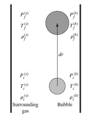
Fig. 7.9 A convective bubble traveling outward a distance dr. Image credit: Carroll & Ostlie (2007).#
According to Archimedes’ principle, if the initial density of the bubble \(b\) is less than its surroundings \(s\) \((\rho_i^{(b)} < \rho_i^{(s)})\), it will begin to rise. The buoyant force per unit volume exerted on a bubble is given by
and the downward gravitational force per unit volume on the bubble is given by
where the net force per unit volume on the bubble becomes
If \(\rho_i^{(b)} < \rho_i^{(s)}\), then \(f_{net} > 0\) (i.e., rising). If the bubble has a greater density than the surrounding material \((\rho_f^{(b)} > \rho_f^{(s)})\), it will sink and convection is prohibited.
To express this condition in terms of temperature gradients, assume that
the gas is initially, very nearly in thermal equilibrium \((T_i^{(b)}\simeq T_i^{(s)}\:\text{and}\:\rho_i^{(b)}\simeq \rho_i^{(s)})\),
the bubble expands adiabatically (i.e., no heat exchange), and
the bubble and surrounding gas pressures are equal at all times \((P_f^{(b)} = P_f^{(s)})\).
If the bubble moves an infinitesimal distance, then it is possible to express the final quantities in terms of the initial quantities and gradients by using a Taylor expansion. To first order,
where the superscript \(x\) represents the bubble \(b\) or the surrounding gas \(s\). If the densities (inside and outside the bubble) remain nearly equal, then for convection we have
Our measurements are mainly of the surroundings and thus, we want to express the density gradient in terms of its surroundings. Using. Eqn. (7.57) for the adiabatically rising bubble allows us to rewrite the LHS of Eqn. (7.62). Assuming that the mean molecular weight is constant as the bubble rises, we use Eqn. (7.55) to rewrite the RHS of Eqn. (7.62), we find
Since the gas pressure is equal at all times, then
and by substitution (and cancellation), we have
Then, we arrive at the requirement
which is now expressed in terms of the actual temperature gradient of the surrounding gas. Notice that Eqn. (7.63) is similar to Eqn. (7.58), where solving for the temperature gradients produces
which is the condition for the temperature gradient of the gas bubble to keep rising.
Another condition for convection can be derived in terms of the change in both pressure and temperature. Using Eqn. (7.63), it can be rewritten as
which may be simplified to
or for convection to occur,
For an ideal monatomic gas \(\gamma = 5/3\) and the RHS of Eqn. (7.65) is 2.5. Once \(d\ln P/d\ln T\) is greater than 2.5, then the region is stable against convection. In general, convection will occur when
the stellar opacity is large, implying that an unattainable steep temperature gradient would be necessary for radiative transport,
a region exists where ionization is occurring, causing a large specific heat and low adiabatic temperature gradient, and
the temperature dependence of the nuclear energy generation rate is large, causing a steep radiative flux gradient and a large temperature gradient.
For stellar atmospheres, the first two conditions occur occur simultaneously and the third condition occurs deep in stellar interiors. In particular, the third condition occurs when the CNO cycle or triple alpha processes are occurring.
7.4.10. The Mixing-Length Theory of Superadiabatic Convection#
In Sect. 7.4.8, we asserted that the temperature gradient must be only slightly superadiabatic and herein, we will justify that assertion. The fundamental criterion for convection requires that the density of a bubble is less than the density of its surroundings. Since the pressure of the bubble and its surroundings are always equal, the ideal gas law implies that the temperature inside the bubble must be larger than its surroundings. The temperature of the surrounding gas mus decrease more rapidly with radius, so
is required for convection (i.e., the temperature of the surroundings is dropping faster than inside the bubble). Since the temperature gradients are negative, we have
Let the temperature gradient of the bubble vary adiabatically and the surrounding gas follow the actual temperature gradient of the star as
After the bubble travels a small distance \(dr\), its temperature will exceed the temperature of the surrounding gas by
Now assume that a hot, rising bubble travels some (characteristic) distance
before dissipating. After which point, it gives up its excess heat at constant pressure. The distance \(\ell\) is called the mixing length and \(H_P\) is the pressure scale height. The ratio of mixing length to the pressure scale height \(\alpha \equiv \ell/H_P\) is an adjustable (or free) parameter generally assumed to be ~1 (values of \(0.5<\alpha <3\) are typical). After the bubble travels one mixing length, the excess heat flow per unit volume from the bubble into its surroundings is
where \(\ell = dr\). Multiplying by the average velocity \(\overline{v}_c\) of the convective bubble, we obtain the convective flux \(F_c\),
Note that \(\rho \overline{v}\) is mass flux, which is a quantity often encountered in fluid mechanics.
The average velocity \(\overline{v}\) can be obtained from the net force per unit volume \(f_{net}\) acting on the bubble. From the ideal gas law (assuming constant \(\mu\)), we have
Since pressure inside and outside the bubble is equal, \(\delta P = 0\) and
From the net force,
We assumed that the initial temperature difference inside and outside the bubble is small \((\delta T_i \approx 0)\) and the buoyant force mus also be small. Since \(f_{net}\) increases linearly with \(\delta T\), we can average over the distance \(\ell\) between initial and final positions, or
Neglecting viscous forces, the work done per unit volume is the net force acting over \(\ell\), or
by the work-energy theorem. Choosing an average kinetic energy over one mixing length leads to some average value of \(\beta v^2\), where \(\beta\) has a value between 0 and 1. Now the average bubble velocity is
Substituting the full expression for \(\langle f_{net}\rangle\) with \(dr = \ell\), we have
using the ideal gas law and definition of the pressure scale height. Through some more manipulation, we can obtain the convective flux
The derivation leading to the convective flux is known as mixing-length theory, which is generally quite successful in predicting the results of observations.
To evaluate \(F_c\), we need to know the difference between the temperature gradients inside and outside of the bubble. Suppose that all of the flux is carried by convection so that,
with the luminosity \(L_r\) at a given radius \(r\). This will allow us to estimate the difference in temperature gradients by rearranging Eqn. (7.68),
Dividing Eqn. (7.69) by the adiabatic temperature gradient (Eqn. (7.60)) gives an estimate for how superadiabatic the actual temperature gradient must be to carry all of the flux by convection alone:
Exercise 7.7
What is the characteristic adiabatic temperature gradient of the Sun’s convection zone? To what degree is the actual gradient superadiabatic? What is the convective bubble velocity?
Starting with a number of assumptions: \(\alpha = 1\), \(\beta = 0.5\), the mass at the base of the convection zone \(M_r = 0.976\,M_\odot\), \(L_r = 1\,L\odot\), \(r=0.714\,R_\odot\), \(g=525\,{\rm m/s^2}\), \(P = 5.59 \times 10^{12}\:{\rm N/m^2}\), \(\rho = 187\:{\rm kg/m^3}\), \(\mu = 0.606\), and \(T = 2.18 \times 10^6\:{\rm K}\). Then from Eqn. (7.60) (adiabatic temperature gradient)
and from Eqn. (7.69)
The relative amount by which the actual temperature gradient is superadiabatic is
The convective velocity needed to carry all of the convective flux is
from scipy.constants import R,G,pi,k
import numpy as np

M_sun = 1.989e30 #mass of the Sun in kg
R_sun = 6.955e8 #radius of the Sun in m
L_sun = 3.827e26 #luminosity of Sun in W
m_H = 1.6735575e-27 #mass of hydrogen in kg

#parameters at the base of convection zone
alpha = 1
beta = 0.5
M_r = 0.976*M_sun #Mass of the Sun in kg
r_c = 0.714*R_sun #Radius of Sun in m
rho = 187 #stellar density  in kg/m^3
g = G*M_r/r_c**2 #local acceleration from gravity in m/s^2
mu = 0.606 #mean molecular weight
T = 2.18e6 #temperature in K
P = 5.59e12 #Pressure in N/m^2
gamma = 5./3.

C_p = gamma/(gamma-1)*(k/(mu*m_H))
dT_dr = g/C_p
print("The adiabatic temperature gradient of the Sun is %1.3f K/m." % dT_dr)

F_c = L_sun/(4*pi*r_c**2)
mu_mH_over_k = mu*m_H/k
bot_fact = alpha**2*np.sqrt(beta)*rho*C_p
delta_T = (g/T)*(F_c*mu_mH_over_k**2/bot_fact)**(2./3.)
print("The difference in temperature gradients is %1.1e K/m" % delta_T)
print("The relative amount by which the actual temperature is superadiabatic is %1.1e." % (delta_T/dT_dr))

v_c = np.sqrt(beta*T*delta_T/g)*(k*alpha/(mu*m_H))
print("The convective velocity is %2d m/s" % np.round(v_c,-1))
The adiabatic temperature gradient of the Sun is 0.015 K/m.
The difference in temperature gradients is 6.7e-09 K/m
The relative amount by which the actual temperature is superadiabatic is 4.4e-07.
The convective velocity is 50 m/s
The mixing length theory can solve some problems, but it is incomplete. The free parameters \(\alpha\) and \(\beta\) must be known a priori (or a least estimated) and they may even vary throughout the star. The time-independent mixing length theory is unsatisfactory when there are stellar pulsations, where the outer layers are oscillating on a timescale comparable to convection \(t_c = \ell/\overline{v}_c\). Rapid changes in the star directly couple to the driving of convective bubbles, which in turn alters the stellar structure.
7.5. Stellar Model Building#
7.5.1. A Summary of The Equations of Stellar Structure#
For your convenience, the basic time-independent stellar structure equations are summarized:
The temperature gradient can depend on the radiation constant \(a=4\sigma/c\) and the average opacity \(\overline{\kappa}\) in radiation dominated environments. The convective (adiabatic) temperature gradient can be applied when
If the star is static (i.e., no radial oscillations), then \(\epsilon = \epsilon_{nuclear}\). Otherwise the energy contribution due to gravity must be included as \(\epsilon = \epsilon_{nuclear} + \epsilon_{gravity}\). The gravitational energy term adds an explicit time dependence to the equations, which can be see through the virial theorem that requires one-half of the gravitational potential energy is lost due to heat.
7.5.2. Entropy#
The gravitational energy generation rate can be expressed in terms of the change in entropy \(S\) per unit mass (the specific entropy) by
and \(\epsilon_{gravity} = -\delta Q/dt\). Then the energy rate is due to the change in entropy directly by
If the star is collapsing, \(\epsilon_{gravity}\) is positive and otherwise it will be negative. As the star contract, its entropy decreases. A star is not a closed system, where its entropy may decrease locally while the entropy of the universe increases due to radiation and stellar wind.
7.5.3. The Constitutive Relations#
The basic stellar structure equations require information regarding the physical composition of the star. The required conditions are the equation of state and are collectively called constitutive relations. These are defined in general as
The pressure equation of state can be quite complex in the deep interior, where the density and temperature are extremely high. However, the ideal gas law (combined with the expression for radiation pressure) is a good first approximation.
The opacity of stellar material cannot be expressed exactly by a single formula. Stellar-structure codes either interpolate a density-temperature grid or use a “fitting function” based on tabulated values. No accurate fitting function can be constructed to account for bound-bound opacities.
The nuclear reaction generation rate can be calculated using formulas for the pp chain and the CNO cycle. Reaction networks are employed to yield individual reaction rates for each step of a process and equilibrium abundances for each isotope in the mixture.
7.5.4. Boundary Conditions#
The actual solution of the stellar structure equations require appropriate boundary conditions that specify how the star should behave between the radiation and convection dominated zones. Boundary conditions tell astronomers the appropriate limits of integration. The central boundary conditions are that the interior mass and luminosity approach zero at the center of the star or
This means that the star does not contain a hole, a core of negative luminosity, or singularities.
A second set of boundary conditions are imposed at the surface of the star, where the temperature, pressure, and density must approach zero, or
The conditions for the surface boundary conditions will never be satisfied exactly for a real star (e.g, the corona). It is often necessary to use more sophisticated surface boundary conditions, such as a star that is losing mass or has an extended atmosphere.
7.5.5. The Vogt-Russell Theorem#
Given the stellar structure equations, constitutive relations (i.e., equation of state), and boundary conditions, we can specify the type of star to be modeled. But, let’s summarize how everything is connected.
The pressure gradient depends on the interior mass and density.
The radiative temperature gradient depends on the local temperature, density, opacity, and interior luminosity.
The luminosity gradient function depends on the density and energy generation rate (depends on density temperature and local composition).
Suppose the entire stellar mass, composition, stellar radius, and luminosity are specified, then the pressure, mass, temperature, and luminosity at an infinitesimal distance \(dr\) (i.e., depth) below the stellar surface can be determined through numerical integration. Starting from the surface and integrating radially towards the center must result in agreement with the central boundary conditions. The values of the various gradients are directly related to the stellar composition and it is not possible to specify an arbitrary combination of radius and luminosity after the mass and composition have been selected. This set of constraints is called the
Vogt-Russell Theorem
The mass and the composition structure throughout a star uniquely determine its radius, luminosity, and internal structure, as well as its subsequent evolution.
The dependence of a star’s mass and composition evolution is a consequence of the change in composition due to nuclear burning (i.e., fusion). There are other factors (e.g., magnetic fields and rotation) that influence stellar interiors, but these are assumed to have little effect in most stars.
7.5.6. Numerical Modeling of the Stellar Structure Equations#
A special family of approximate solutions to the stellar structure are known as polytropes, but the system of differential equations for the stellar structure cannot be solved analytically for all cases. Therefore it is necessary to evaluate the differential equations numerically by approximating the equations by difference equations (by replacing \(d\) with \(\Delta\) in the gradients). Then the star is modeled as a set of spherically symmetric shells and the integration is carried out starting from some initial radius (given the initial state) in finite steps by specifying an increment \(\delta r\).
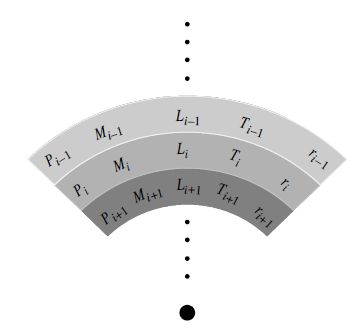
Fig. 7.10 Zoning in a numerical stellar model. The star is assumed to be constructed of spherically symmetric mass shells, with the physical parameters associated with each zone being specified by the stellar structure equations, the constitutive relations, the boundary conditions, and the star’s mass and composition. Image credit: Carroll & Ostlie (2007).#
Note
Codes that treat the radius as an independent variable are called Eulerian, while Lagrangian codes treat the mass as an independent variable. Codes in the Lagrangian formulation have the hydrostatic equilibrium written as \(dP/dM\) instead of \(dP/dr\).
Each shell is solved through successive applications of the difference equations and a successive shell depends recursively on the shell that came before it. For example, the pressure in a given zone \(P_i\) determines the pressure in the next deepest zone \(P_{i+1}\), or
where the integration is progressing inward and \(\delta r < 0\). The numerical integration of the stellar structure can be executed
from the surface towards the center,
from the center towards the surface, or
in both directions simultaneously using boundary conditions.
In the last case there must be some boundary (fitting point) where the variable must vary smoothly from one solution to the other. This approach is frequently taken because the most important physical processes in the outer layers generally differ from the deep interior (i.e., separate radiative and convective zones). The transfer of radiation through optically thin zones and ionization (of hydrogen and helium) occur close to the surface, while nuclear reactions occur near the center.
Simultaneously matching the surface and central boundary conditions for a desired stellar model usually requires many iterations (i.e., series of attempts) before a satisfactory solution is found. If the integrations do not agree at the fitting point, then the starting conditions must be changed.
A very simple stellar structure code (called StatStar) integrates the stellar structure equations in their time independent form from the outside to the center using the appropriate constitutive relations; it also assumes a homogenous composition throughout. Many of the sophisticated techniques and the complex formalism of the mixing length theory are omitted from StatStar in favor of the simplifying assumption of adiabatic convection. Very reasonable models may be obtained for main sequence stars despite the approximations.
7.5.7. Polytropic Models and the Lane-Emden Equation#
Under very special situations, it is possible to find analytic solutions to a subset of the stellar structure equations. The famous equation that helps us describe analytical stellar models is the Lane-Emden equation.
Note
The first work was carried out by J. Homer Lane in 1869. His work was extended significantly by Robert Emden in 1907.
If only a simple relationship existed between pressure and density, then the mechanical equations of stellar structure could be solved simultaneously. However this is not the case in general, where temperature and composition enter into the pressure equation of state. For an adiabatic gas, the pressure can be written explicitly in terms of the density alone. Hypothetical stellar models in which the pressure depends solely on the density are polytropes and are written as a power law, \(P = K \rho^\gamma\). The development of polytropic models provides insight into stellar structure, without the complications of full-blown numerical models.
To derive the Lane-Emden equation, we start with hydrostatic equilibrium and re-write the equation through the radial derivative,
where the mass gradient can be substituted to get
or
The form of Eqn. (7.71) should look familiar as the very well-studied differential equation known as Poisson’s equation and then can be rewritten as
which depends on the gravitational potential energy per unit mass, \(\Phi_g \equiv U_g/m\).
Note
Poisson’s equation shows up frequently in physics, where Gauss’ Law can be reformulated into Poisson’s equation by replacing \(\vec{E}\) with \(-\nabla\Phi_E\).
The equation of a polytrope can now be substituted into Eqn. (7.71), where \(K\) and \(\gamma > 0\) are constants. Through substitution, we get
Letting \(\gamma = (n + 1)/n\), where \(n\) is the polytropic index. Then
Note
Different values of the polytropic index are assumed to model rocky planets, giant planets, hot Jupiters, and stars in reference to the dissipation of tides.
The density can be rewritten in a dimensionless form through the use of a scaling factor and dimensionless function \(D(r)\), let
and the critical central density \(\rho_c\) of the polytropic stellar model. Through additional substitution,
This equation can be simplified if we define
and introduce the dimensionless independent variable \(\xi\) through \(r\equiv \lambda_n \xi\) to get
the famous Lane-Emden equation. The dimensionless function is transformed to \(D_n(\xi)\) for a specific polytropic index \(n\) and leads directly to a density profile \(\rho_n(r)\). The polytropic pressure equation of state is given as \(P_n(r) = K\rho_n^{(n+1)/n}\). The temperature profile can be obtained if the ideal gas law and a constant composition for the radiation pressure are assumed.
To solve the second-order differential equation, two boundary conditions are needed.
Assume that the stellar surface is where the pressure (and gas density) goes to zero and then \(D_n(\xi_1) = 0\) specifies the surface at \(\xi = \xi_1\), which is the first zero of the solution.
Assume there is some distance \(\delta\) that is infinitesimally close to the center of the star, then the mass contained is given by \(M_r = \frac{4}{3}\pi \overline{\rho}\delta^3\),
using the average gas density \(\overline{\rho}\) within the radius \(\delta\). Through substitution into hydrostatic equilibrium, we have
where \(dP/dr \rightarrow 0\) as \(r\rightarrow 0\). Since \(P \propto \rho\), this implies that \(d\rho/dr \rightarrow 0\) as well and leads to the central boundary condition \(D_n(0)/d\xi = 0\). For \(\rho_c\) to represent the central density, the density scaling function \(D_n(0) = 1\) (through normalization).
It is now possible to compute the total mass given a specific polytropic index as
using \(R = \lambda_n \xi_1\) as the stellar radius. Rewriting in terms of dimensionless quantities results in
With knowledge of \(D_n(\xi)\), the above equation could be integrated directly, but it can also rewritten using the Lane-Emden equation as the anti-derivative with the central boundary condition, noting that
and
where the derivative is evaluated at the surface.
There are only three analytic solutions to the Lane-Emden equation \((n = 0,\,1,\,{\rm and}\,5)\). These solutions are
The \(n=1\) solution is the well-known “sinc” function.
import matplotlib.pyplot as plt
import numpy as np

def density_scaling_func(n,xi):
    D_n = -np.ones(len(xi))
    if n == 0:
        D_n = 1-xi**2/6
    elif n==1:
        sinc = np.sin(xi[1:])/xi[1:]
        sinc_rng = np.where(np.logical_and(xi<=np.pi,xi>0))[0]
        D_n[sinc_rng] = sinc[sinc_rng]
        D_n[0] = 1.
    elif n==5:
        D_n = 1./np.sqrt(1+xi**2/3.)
    return D_n

aspect = 1
width = 5
fs = 'large'

xi = np.arange(0,10,0.01) #range in xi

fig = plt.figure(figsize=(aspect*width,width),dpi=150)
ax = fig.add_subplot(111)

ax.plot(xi,density_scaling_func(0,xi),'k-',lw=2,label="$D_0$")
ax.plot(xi,density_scaling_func(1,xi),'k--',lw=2,label="$D_1$")
ax.plot(xi,density_scaling_func(5,xi),'k:',lw=2,label="$D_5$")

ax.legend(loc='best',fontsize=fs)

ax.set_xlabel("$\\xi$",fontsize=fs)
ax.set_ylabel("$D_n(\\xi)$",fontsize=fs)
ax.set_xlim(0,10)
ax.set_ylim(0,1);
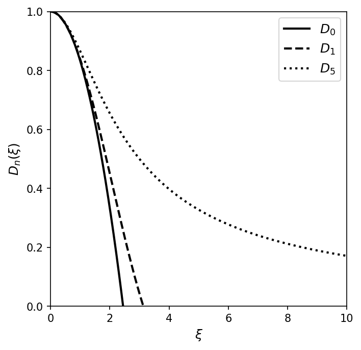
The discussion of polytropes arose by the equation of state for an adiabatic gas. For the case of an ideal, monatomic gas \(\gamma=5/3\) which implies \(n=1.5\). Certain extremely compressed stars known as white dwarfs can also be described using \(n=1.5\), although these are non-relativistic, completely degenerate stars. Note that this case must be solved numerically.
The Eddington standard model associated with a star in radiative equilibrium uses \(n=3\). Consider a polytrope that is supported by both an ideal gas and radiation pressure. If the total pressure at a given radius \(P\) is supplied, the pressure of the gas is given by
where the factor \(\beta\) is a number between 0-1, then the contribution due to radiation pressure is
We are looking for a polytropic equation of state independent of temperature. Using Eqn. (7.74), we have
and by substitution we obtain
which leads to polytropic expression
by bundling the constants into
With \(\gamma = 4/3\), then \(n=3\) and describes stars that are supported by a fully relativistic, completely degenerate gas (i.e., neutron stars).
7.6. The Main Sequence#
The analysis of stellar spectra shows that the atmospheres of most stars are composed primarily of hydrogen \((X\sim 0.7)\), whereas the fraction of metal varies \((0< Z < 0.03)\). If the initial stellar composition is homogenous, then the first set of nuclear reactions should be the pp chains and/or the CNO cycle because they convert hydrogen into helium. The core of a star is predominantly hydrogen and the stellar interior will evolve slowly due to the nuclear reactions. Most stars have similar compositions and thus, stellar structure should smoothly vary with mass. This is apparent when we see the central pressure and temperature increasing along with the total mass.
For low mass stars the pp chain will dominate because it doesn’t have enough gravity to overcome the Coulomb barrier of heavier nuclei. For high mass stars, the CNO cycle will likely dominate because of its strong temperature dependence. For progressively less massive stars, the central temperature will eventually fall below the critical point for fusion and are no longer able to stabilize the star against gravitational contraction. This critical point depends on the stellar metal mass fraction, where \(0.072\:M_\odot\) is for solar composition and metal free stars (\(Z=0\)) the value climbs to \(0.09\:M_\odot\). For extremely massive stars \((\ge 90\:M_\odot)\) thermal oscillations in the core may produce significant variations that affect the nuclear energy generation rate.
7.6.1. The Eddington Luminosity Limit#
The stability of vey massive stars is directly affect by their extremely high luminosities. If the temperature is sufficiently high and gas density is low, then it is possible for the radiation pressure to dominate over the gas pressure. When this occurs in the outer portions of very massive (or large) stars, the outer layers can disperse due to the intense stellar wind. Using the conditions for radiant flux and luminosity, the pressure gradient near the stellar surface is
But the pressure gradient is related to the local gravity \(dP/dr = -g\rho\). Combining and solving for luminosity, we have
The maximum radiative luminosity \(L_{\rm Ed}\) (or Eddington limit) is a maximum value for a star to remain in hydrostatic equilibrium. If \(L>L_{\rm Ed}\), then mass loss must occur that is driven by radiation pressure.
It is possible to estimate the Eddington luminosity for stars on the upper end of the main sequence (i.e., very hot and bright). The effective temperatures of these stars are ~50,000 K, where most of the hydrogen is ionized in the photosphere. The major contribution to the opacity is from electron scattering \(\overline{\kappa}_{es}\),
or
from scipy.constants import G,c,pi

M_sun = 1.989e30 #mass of the Sun in kg
L_sun = 3.846e26 #luminosity of the Sun in W
X = 0.7
L_ed = 200*pi*G*c/(1+X)*M_sun
print("The Eddington limit for X=0.7 is %1.1e W." % L_ed)
print("The Eddington limit relative to a solar luminosity is %1.1e." % (L_ed/L_sun))
The Eddington limit for X=0.7 is 1.5e+31 W.
The Eddington limit relative to a solar luminosity is 3.8e+04.
For a \(90\:M_\odot\) star, \(L_{\rm ed} \simeq 3.5\times 10^6\:{L_\odot}\) and is roughly three times the expected main-sequence value.
7.6.2. Variations of Main-Sequence Stellar Parameters with Mass#
From theoretical models computed in the mass range of hydrogen burning, it is possible to obtain a numerical \(M-L\) relationship that agrees well with the observational \(M-L\) relationship. Stars undergoing hydrogen burning in the cores lie along the observational main sequence. The range in main-sequence luminosities range from \(5\times 10^{-4}\:L_\odot\) to \(1 \times 10^6\:L_\odot\); a variation of nine orders of magnitude, while the masses change by only three orders of magnitude. Due to the higher energy output from upper main-sequence stars, they consume their core hydrogen quicker. Therefore, main-sequence lifetimes decrease with increasing luminosity. Effective temperature are much less dependent on stellar mass because they are determined from the photosphere, not the core. However the variation is still large enough to dramatically change the stellar spectrum.
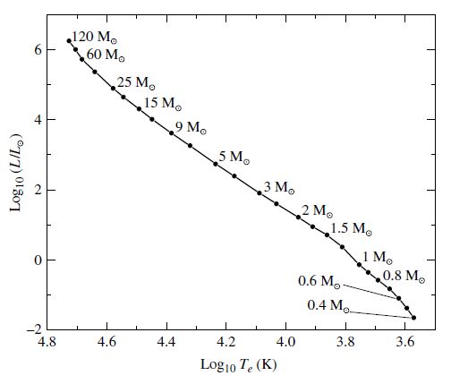
Fig. 7.11 The locations of stellar models on a theoretical H–R diagram. Image credit: Carroll & Ostlie (2007).#
The interior structure of stars along the main sequence stars also varies with mass, primarily in the location of convection zones. For stars that produce energy mainly through the CNO cycle, convection is dominant in the core. Outside of the core, radiation is capable of transporting the flux and convection ceases. At ~1.2 \(M_\odot\), the pp chain begins to dominate and the core becomes radiative. Meanwhile the stellar surface cools with decreasing mass and the opacity increases because (in part) by the location of the hydrogen ionization zone. The increased opacity makes convection more efficient near the surface. The bottom of the surface convection zone grows deeper until the entire star becomes convective near 0.3 \(M_\odot\).
7.7. Homework#
Problem 1
Show that the equation for hydrostatic equilibrium (Eqn. (7.7)) can also be written in terms of the optical depth \(\tau\), as
Problem 2
Derive the ideal gas law in Eq. (7.10) starting from the pressure integral and the Maxwell-Boltzmann distribution function.
Problem 3
The \(Q\) value of a reaction is the amount of energy released (or absorbed) during the reaction. Calculate the \(Q\) value for each step of the PP I chain. Express your answers in MeV. The masses of deuterium and helium-3 are 2.0141 u and 3.0160 u, respectively.
Problem 4
Complete the following reaction sequences. Be sure to include any necessary leptons.
(a) \({^{27}_{14}{\rm Si}} \rightarrow {^?_{13}{\rm Al}} + e^+ + ?\)
(b) \({^{?}_{13}{\rm Al}} + {^1_1{\rm H}} \rightarrow {^{24}_{12}{\rm Mg}} + {^4_?{\rm ?}}\)
(c) \({^{35}_{17}{\rm Cl}} + {^1_1{\rm H}} \rightarrow {^{36}_{18}{\rm Ar}} + ?\)
Problem 5
Prove that \(P = K^\prime T^{\gamma/(\gamma-1)}\) follows from \(PV^\gamma =K\).
Problem 6
Estimate the hydrogen burning lifetimes of stars near the lower and upper ends of the main sequence.
(a) The lower end of the main sequence occurs near 0.072 \(M_\odot\), with \(\log_{10}\,T_e = 3.23\) and \(\log_{10}(L/L_\odot)=-4.3\). Assume that the star is entirely convective so that all of its hydrogen becomes available for burning through convective mixing.
(b) An 85 \(M_\odot\) star (with only 10% of the hydrogen available) near the upper end of the main sequence has an effective temperature and luminosity of \(\log_{10}\,T_e = 4.705\) and \(\log_{10}(L/L_\odot)=6.006\), respectively.
Problem 7
Using the information in problem 6, calculate the radii of each star. What is the ratio of their radii?
7.8. Additional Resources#
Another textbook for stellar astrophysics is available from Edward Brown at Michigan State, which covers some material in greater depth.