6. The Sun

6.1. The Solar Interior

6.1.1. The Evolutionary History of the Sun

Our Sun is classified as a typical main-sequence star of spectral class G2, which contains mostly hydrogen \((X=0.74)\), some helium \((Y=0.24)\), and a little metal (\(Z=0.02)\) by mass. The composition has changed (evolved) over time because it has been converting hydrogen into helium through the proton-proton chain for most of its lifetime. Even though the Sun is changing over time, we can still estimate its age using other bodies of the Solar System. For example, radioactive dating of Moon rocks and meteorites indicate that they are ~4.57 Gyr old and the Sun would be at least as old as these rocks. Since becoming a main-sequence star, the Sun’s luminosity has increased by nearly 48% and its radius has increased by 15%, which lead to an increase a 2.7% increase in its effective temperature. The effect of this luminosity increase on the Earth is unclear due to the Earth’s time-varying ability to reflect light through its albedo (caused by surface water and ice).

Note

Radioactive dating of the oldest known objects in the Solar System, the calcium-aluminum inclusions (CAIs), indicates that the age of the Solar System is \(4.56730 \pm 0.00016\) Gyr, or \(4567.30 \pm 0.16\) Myr.

6.1.2. The Present-Day Interior Structure of the Sun

Using the current age of the Sun, a solar model must reproduce the current values of the central temperature, pressure, density, and composition. A schematic of the Sun can be constructed, where an inner core produces the radiation through nuclear reactions, a middle layer transports the energy through radiation, and an outer atmosphere brings energy to the surface through convection cells of rising and sinking gas. Using such a model, the hydrogen mass fraction \((X)\) in the core has decreased from 0.71 to 0.34 and the helium mass fraction increased from 0.27 to 0.64 over the Sun’s lifetime. At the surface the hydrogen mass fraction increased by 0.03, while the helium mass fraction decreased by 0.03.

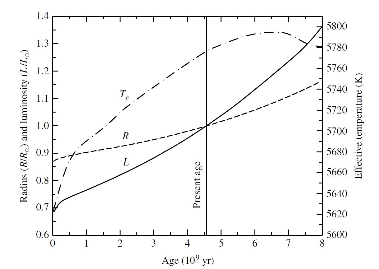
Fig. 6.1 The evolution of the Sun on the main sequence. As a result of changes in its internal composition, the Sun has become larger and brighter. The solid line indicates its luminosity, the dashed line its radius, and the dash-dot line its effective temperature. The luminosity and radius curves are relative to present-day values. Image credit: Carroll & Ostlie (2007); data are from Bahcall, Pinsonneault, and Basu (2001).

Evolution of the Sun’s interior includes ongoing nucleosynthesis, surface convection, and elemental diffusion (settling of heavier elements). The Sun’s primary energy production comes from the proton-proton (pp) chain, where \(^3{\rm He}\), or tritium is an intermediate species in the reaction sequence. Tritium can be produced and destroyed as part of the conversion of hydrogen into helium. However, tritium is relatively more abundant at the top of the hydrogen-burning region where the temperature is lower. At greater depths, the higher temperatures the destroy the tritium more often than it is created, resulting in a overall decrease in abundance. The production of \(^4{\rm He}\) (stable helium) decreases and hydrogen increases slightly near 0.7 \({\rm R_\odot}\) due to the surface convection zone and elemental diffusion.

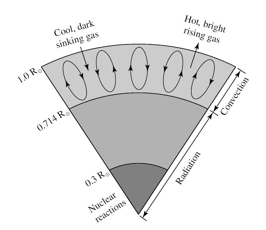
Fig. 6.2 A schematic diagram of the Sun’s interior. Image credit: Carroll & Ostlie (2007).

Table 6.1 Central Conditions in the Sun. (Data are from Bahcall, Pinsonneault, and Basu (2001)).

Parameter	Value
Temperature	\(1.570 \times 10^7\ {\rm K}\)
Pressure	\(2.343 \times 10^{16}\ {\rm N/m^2}\)
Density	\(1.527 \times 10^5\ {\rm kg/m^3}\)
X	0.3397
Y	0.6405

The largest contribution to the energy production occurs at approximately 0.1 \({\rm R_\odot}\), as seen in the radial derivative of the luminosity profile as a function of radius. Consider the mass conservation equation

(6.1)\[\begin{align} \frac{dM_r}{dr} = 4\pi r^2 \rho \; \rightarrow \; dM_r = 4\pi r^2 \rho\:dr = \rho\:dV, \end{align}\]

which indicates how the mass within a certain radius interval increases because the volume of a spherical shell increases with a fixed choice of \(dr\). Even if the total energy liberated per kilogram of material \((\epsilon)\) decreases steadily from the inside-out, then the largest contribution to the total luminosity will occur in a shell that contains a significant mass rather than at the center. In the case of the current (middle-aged) Sun, the decrease in available hydrogen fuel at the center will also influence the location of the peak energy production. The pressure and density can change rapidly with radius, which produces variations on the solar structure through conditions of hydrostatic equilibrium, ideal gas law, and the composition structure.

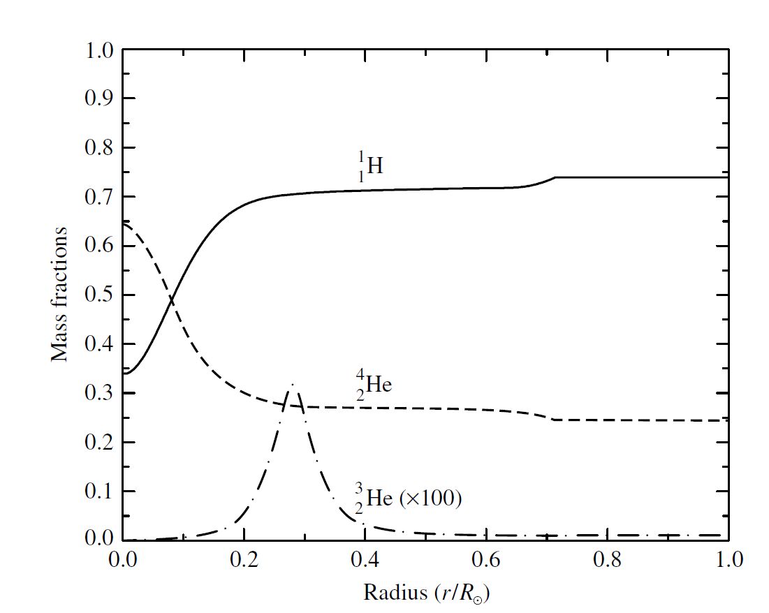
Fig. 6.3 The abundances of \(^1_1{\rm H}\), \(^3_2{\rm He}\), and \(^4_2{\rm He}\) as a function of radius for the Sun. Note that the abundance of \(^3_2{\rm He}\) is multiplied by a factor of 100. Image credit: Carroll & Ostlie (2007); data are from Bahcall, Pinsonneault, and Basu (2001).

The interior mass as a function of radius \((M_r)\) shows that 90% of the Sun’s mass lies within roughly 0.5 \({\rm R_\odot}\). The interior mass function can be determined through the integration of the density function over the Sun’s volume (i.e., \(M_r = \int \rho\:dV\)). The energy generated in the interior has to be transported outwards, where a criterion for the onset of convection is that the temperature gradient becomes superadiabatic,

\[ \left|\frac{dT}{dr}\right|_{\rm actual} > \left|\frac{dT}{dr}\right|_{\rm adiabatic}, \]

where actual and adiabatic refer to the temperature gradients. For an ideal monatomic gas, this conditions becomes,

\[ \frac{d\ln P}{d\ln T} < 2.5. \]

The Sun is purely radiative below 0.714 \({\rm R_\odot}\) and is convective above that point. This occurs because the opacity in the outer layer becomes large enough to block the energy transport by radiation. For a large temperature gradient, convection becomes the more efficient means of energy transport. A rapid rise in \(d\ln P/ d\ln T\) near the surface \((r>0.95\:{\rm R_\odot})\) is due to the significant departure of the actual temperature gradient from an adiabatic one.

Note

Stars need only be slightly more massive than the Sun in order to be convective at their centers because of the strong temperature dependence of the CNO cycle as compared to the pp chain.

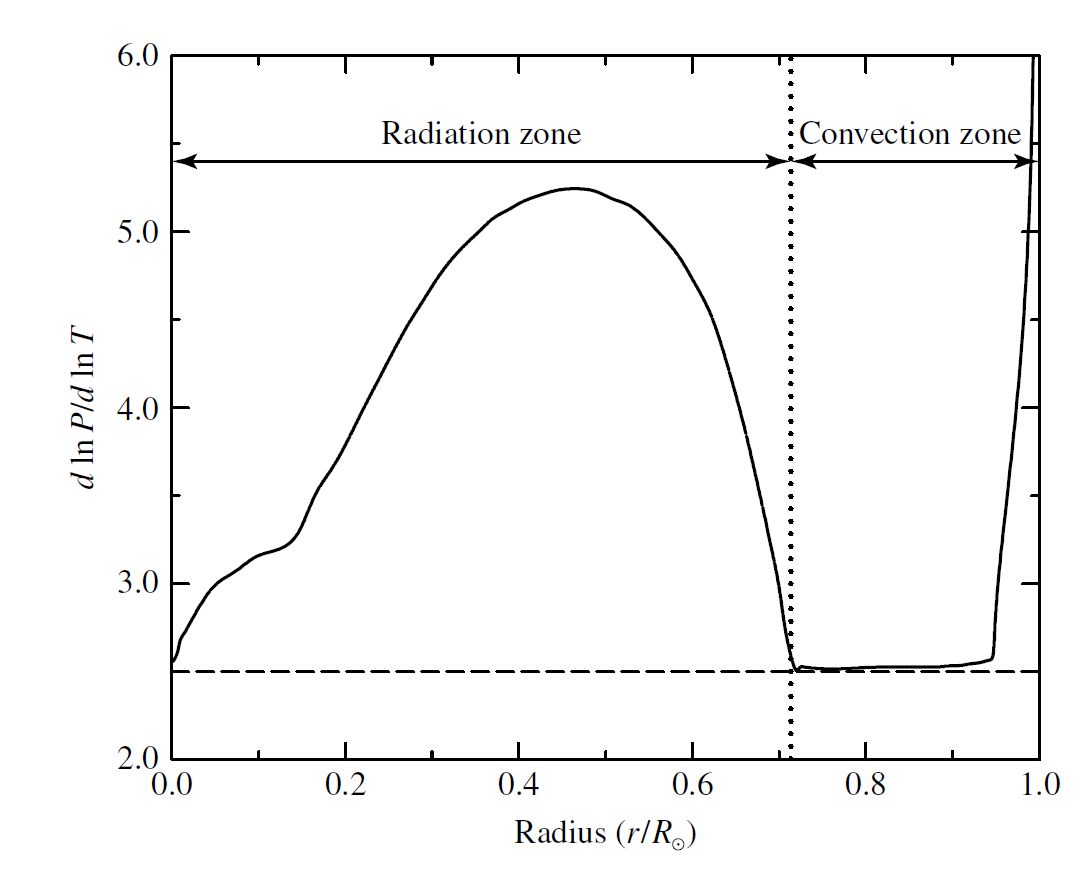
Fig. 6.4 The convection condition \(d \ln P/d \ln T\) plotted versus \(r/R_\odot\). Image credit: Carroll & Ostlie (2007); data are from Bahcall, Pinsonneault, and Basu (2001) and Cox (2000).

Models of stellar structure and the derivation of fundamental physical principles have uncovered an enormous amount of information regarding the Sun’s interior. A complete and reasonable model needs to be consistent with evolutionary timescales and the global characteristics (e.g., mass, luminosity, radius, effective temperature, surface composition, and oscillation frequencies). However there is one aspect of the Sun where the observations don’t match the theoretical model, which is the abundance of lithium. The observed lithium abundance is somewhat less than expected, which may imply that some adjustments (e.g., through convection, rotation, and/or mass loss) to the model are necessary.

6.1.3. The Solar Neutrino Problem: A Detective Story Solved

For decades, there was an inconsistency between the observations of the Sun and the model, where the solution resulting in an important new understanding of fundamental physics. In 1970, Raymond Davis began measuring the neutrino flux from the Sun. His detector was located almost 1 mile below ground within a gold mine in Lead, South Dakota. The neutrino has a very low cross section for interaction with other matter, which makes it difficult to detect. Like the eye of Sauron, neutrinos penetrate where other particles cannot. The detector was placed underground to lower the background noise and ensure that it was only measuring neutrinos.

The neutrino detector contained ~100,000 gallons of cleaning fluid, \({\rm C_2Cl_4}\) (tetrachloroethylene), because chlorine interacts with \({\rm ^{37}_{17}Cl}\) to produce \({\rm ^{37}_{18}Ar}\) that has a half-life of 35 days,

\[ {\rm ^{37}_{17}Cl} + \nu_e \rightleftharpoons {\rm ^{37}_{18}Ar} + e^-.\]

The threshold energy for this reaction is 0.814 MeV and less than the energy of the neutrinos produced in almost every step of the pp chain. The neutrinos in the first step,

\[ {\rm ^1_1H} + {\rm ^1_1H} \rightarrow {\rm ^2_1H} + e^+ + \nu_{e^-}, \]

produced more energy, but the reaction that accounted for 77% of the neutrinos detected is the \(\beta^+\) decay of \({\rm ^8_5 B}\) into \({\rm ^8_4Be}\):

\[ {\rm ^8_5B} \rightarrow {\rm ^8_4Be} + e^+ + \nu_e. \]

Unfortunately, this reaction is very rare (1:5000). Every few months, Davis and his collaborators purged the accumulated argon and determined the number of argon atoms produced. The capture rate was measured using the solar neutrino unit, where 1 SNU equals \(10^{-36}\) reactions per target atom per second. The tank contained \(\sim10^{30}\) \({\rm ^{37}_{17}Cl}\) atoms, which corresponds to 5.35 SNU if only 1 argon atom was produced each day.

John Bahcall computed the anticipated capture rate of 7.9 SNU, while the actual data (taken between 1970 and 1994) yielded an average of \(2.56 \pm 0.16\) SNU. About one-third of the expected yield. Other experiments have confirmed the discrepancy including Japan’s underground Super-Kamiokande observatory. This observatory detects the Cerenkov light produced when neutrinos scatter electrons. Through this measurement only half of the neutrinos are detected compared to the predictions from solar models.

The deficit of neutrinos suggested that either (a) some fundamental physical process in the solar model is incorrect or (b) something happens to the neutrinos in-transit (i.e., on their way from the Sun’s core to the Earth). The Mikheyev-Smirnov-Wolfenstein (or MSW) effect involves transformation of neutrinos between the three types (\(\nu_\mu\), \(\nu_\tau\), and \(\nu_e\)). This idea is an extension of the electroweak theory* fof particle physics.

Confirmation of this idea came in 1998 when Super-Kamiokande was used to detect atmospheric neutrinos produced in Earth’s upper atmosphere. Cosmic rays are capable of producing only electron and muon neutrinos. Super-Kamiokande determined that the number of \(\nu_\mu\) traveling upward was significantly reduced compared to those traveling downward, where the difference in numbers is in excellent agreement with the theory of neutrino mixing. For neutrino mixing to occur, the neutrino could not be a massless particle and the experiment confirmed this as well. After several decades the solar neutrino problem was resolved by a profound advance in our understanding of particle physics.

6.2. The Solar Atmosphere

6.2.1. The Photosphere

Optical photons appear to originate from an outer layer of the Sun called the photosphere. The base of the photosphere is somewhat arbitrary since photons because some photons originate from deep within the Sun (\(\tau_\lambda \gg 1\)). The optical depth from a given layer \(\tau_\lambda\) can be estimated from an estimate of the fraction of photons that we receive from that layer (i.e., \(\tau_\lambda = -\ln\left(I_\lambda/I_{\lambda,o}\right)\)). For instance, if 1% of the photons from a given layer, then the optical depth is approximately 4.6. The opacity and optical depth are wavelength-dependent, where the base of the photosphere is also wavelength dependent if it is defined in terms of the optical depth.

Note

Given the arbitrariness of the definition, the photosphere’s base is sometimes simply defined as 100 km below \(s_1\), the level where the optical depth at 500 nm is unity:

\[ s_1 = \frac{\tau_{500} }{\kappa_{500} \rho} = \frac{1}{\kappa_{500} \rho}. \]

The base of the photosphere is 100 km below \(s_1\), which corresponds to an optical depth \(\tau_{500} \approx 23.6\) and the temperature is approximately 9400 K.

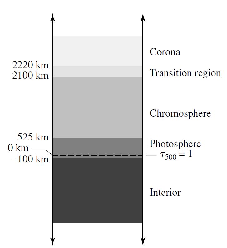
Fig. 6.5 The thicknesses of the components of the Sun’s atmosphere. Image credit: Carroll & Ostlie (2007).

The gas temperature decreases to 4400 K at 525 km above \(s_1\) \((\tau_{500}=1)\) as we move upward from the base and through the solar photosphere. The temperature minimum defines the top of the photosphere, where the temperature begins to rise above this point. The photosphere is defined to be 625 km thick and the bulk resides above an optical depth equal to unity. On average, the solar flus is emitted from and optical depth \(\tau = 2/3\) (the Eddington approximation), which leads to defining the effective temperature (for Wien’s law) at this depth.

A source of opacity exists and is continuous across wavelength due in part to the \(H^-\) ions in the photosphere. Using the Saha equation, we can determine the ratio of \(H^-\) ions to the neutral hydrogen atoms. The abundance of H II \((H^-\:{\rm ions})\) in the Sun is actually quite low (1 in \(10^7\) atoms), but it becomes important because neutral hydrogen is not capable of contributing significantly to the continuum.

An individual spectral line is not infinitesimally thin covering a range of wavelengths and different parts of the same line can originate form at different depths of the solar atmosphere. The absorption lines (e.g., Fraunhofer lines) are produced in the photosphere.

From Kirchoff’s laws, the absorption lines are produced when there is a cooler gas between the observer and the bulk of the hot source (i.e., continuum-forming region). In reality, the Fraunhofer lines are formed in the same layers where \(H^-\) ions produce the continuum. The center of an absorption line originates from the regions of lower optical depth (i.e., higher in the photosphere) where the gas is cooler because the opacity is greatest at the center of the line (i.e., more difficult to see deeper in the atmosphere). Moving into the wings of the line, the opacity decreases and this implies that absorption is occurring at progressively deeper levels. At wavelengths far from the central line, the absorption is negligible and the continuum is observed.

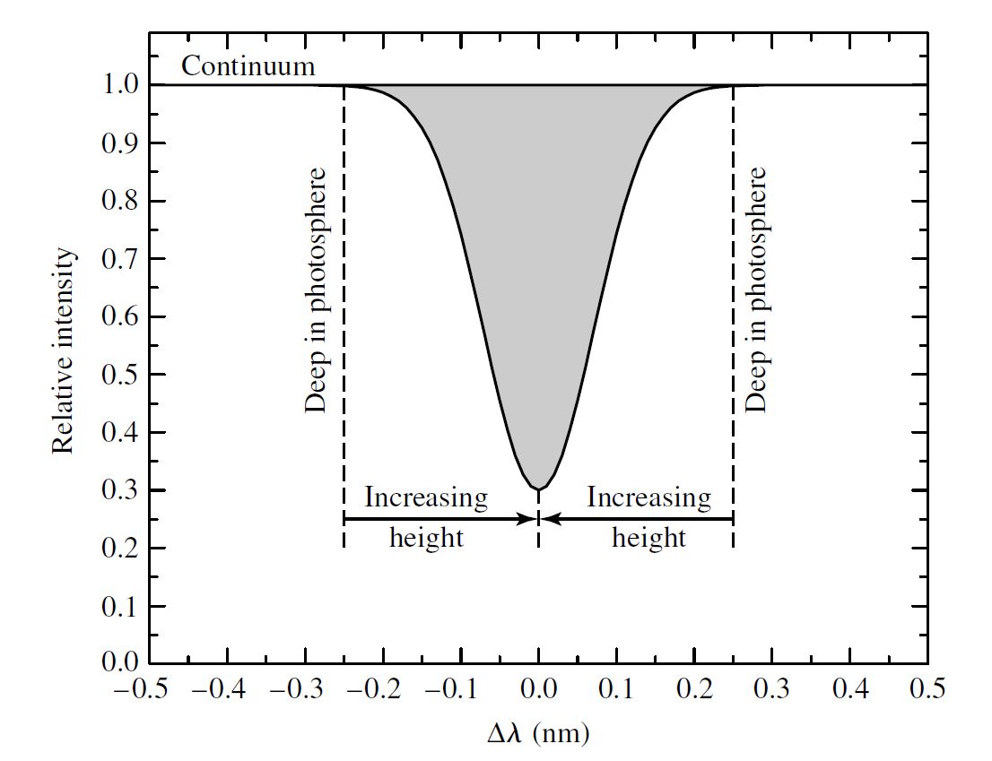
Fig. 6.6 The relationship between absorption line strength and depth in the photosphere for a typical spectral line. The wings of the line are formed deeper in the photosphere than is the center of the line. Image credit: Carroll & Ostlie (2007).

6.2.1.1. Solar Granulation & Differential Rotation

Observations of the photosphere show a patchwork of bright and dark regions evolve over time, where the dark regions can appear and then disappear. The spatial extent of a region can be 700 km and have a lifetime for 5-10 minutes. This structure is called granulation and represents the top portion of a convection zone protruding into the photosphere’s base. Granulation causes wiggles to appear in the absorption lines due to small Doppler shifts (400 m/s) from the convection cycle. The brighter regions produce blueshifts (i.e., rising hot material) in the absorption lines while the darker regions are caused by redshifts (i.e., sinking cool material). The lifetime of a granule is defined as the amount of time for a parcel to rise and fall the distance of one mixing length.

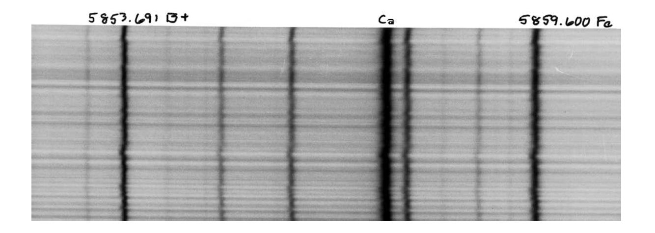
Fig. 6.7 A spectrum of a portion of the photospheric granulation showing absorption lines that indicate the presence of radial motions. Wiggles to the left are toward shorter wavelengths and are blueshifted while wiggles to the right are redshifted. Image credit: Carroll & Ostlie (2007).

The absorption lines are used to measure the rotation rate of the Sun, where measurements are taken from the equator and then outward with increasing latitude. By measuring Doppler shifts as a function of latitude, we find that the Sun rotates differentially meaning the rotation rate changes with latitude. The rotation period at the equator is approximately 25 days, while it increases to 36 days at the poles. The Sun’s rotation also varies internally with radius. Near the base of the convection zone, differing rotation rates converge into a region known as a tachocline. The differing rotation rates produce a strong shear in the atmosphere, which can result in electric currents in the plasma that generate the Sun’s magnetic field.

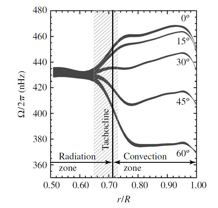
Fig. 6.8 The rotation period of the Sun varies with latitude and depth. The angular frequency \(\Omega\) has units of radians per second. Image credit: Carroll & Ostlie (2007).

6.2.2. The Chromosphere

Above the photosphere lies a portion of the Sun’s atmosphere called the chromosphere that is only about 0.01% (or a factor of \(10^{-4}\)) of the photosphere’s intensity and extends upward for approximately 1600 km or 2100 km above \(\tau_{500} = 1\). The light produced in the chromosphere indicates that the gas density drops dramatically (by a factor of \(10^4\)) and the temperature begins to increase with altitude, from 4400 K to 10,000 K. The Boltzmann and Saha equations show that spectral lines can be produced in the low density and high temperature environment of the chromosphere (e.g., He II, Fe II, Si II, Cr II, and Ca II).

Certain Fraunhofer lines appear as absorption lines in the visible and near-UV, where others begin to appear as emission lines at shorter (or much longer) wavelengths. Kirchoff’s laws suggest that a hot, low-density gas must be responsible for the emission lines. The emission cannot occur deep within the Sun’s interior because the Sun is optically thick and so the area of emission line production occurs elsewhere. The strength of the continuum decreases rapidly at shorter and longer wavelengths (far from the peak at 500 nm). Thus, emission lines produced far from the visible are not overwhelmed by the expected blackbody radiation.

Emission lines (in the visible range) are observable near the limb of the Sun for a few seconds when the bright solar disk is occulted during a total eclipse and is known as a flash spectrum. During an eclipse the Sun gaines a reddish hue because the Balmer \({\rm H\alpha}\) emission line can now dominate. Alternatively, filters can be used to restrict observations to the wavelengths of emission lines in the chromosphere (particularly \({\rm H \alpha}\)) and a great deal of hidden structure becomes visible. On scales of 30,000 km, the continued effects of the convection zone are seen as supergranulation. Similar to granules, Doppler studies reveal the rising and sinking of gas at 400 km/s. Spicules, or vertical filaments of gas, are present that extend upward for 10,000 km and each spicule has a lifetime of only 15 minutes. As a result the speed of particles in spicules move upwards at approximately 15 km/s, as shown through Doppler studies.

6.2.3. The Transition Region

The temperature rises rapidly within approximately 100 km above the chromosphere and reach \(>10^5\) K before \(dT/dr\) begins to flatten. The temperature still increases, but more slowly until eventually exceeding \(10^6\) K. Selective observations in the UV and extreme-UV reveal this transition region. Lyman-alpha (or \({\rm Ly\alpha}\)) hydrogen emission (\(2\rightarrow 1\)) is produced when the temperature reaches 20,000 K (at the top of the chromosphere), the C III emission line originates when the temperature reaches 90,000 K, the O VI line occurs at 300,000 K, and the Mg X line occurs at \(1.4 \times 10^6\) K.

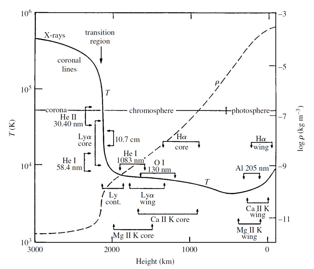
Fig. 6.9 Logarithmic plots of the temperature structure (solid line) and mass density structure (dashed line) of the upper atmosphere of the Sun. Image credit: Carroll & Ostlie (2007).

6.2.4. The Corona

During a total solar eclipse, a faint corona appears around the Sun at totality. The corona lies above the transition region, extends out into space without a well-defined outer boundary, and is very faint (about \(10^6\) times less intense) compared to the photosphere. The number density of particles at the corona’s base is \(\sim 10^{15}\:{\rm particles/m^3}\), whereas the Solar wind has a number density of particles of \(\sim 10^7\:{\rm particles/m^3}\) in the vicinity of Earth and the number density of particles in Earth’s atmosphere at sea level is \(\sim 10^{25}\:{\rm particles/m^3}\).

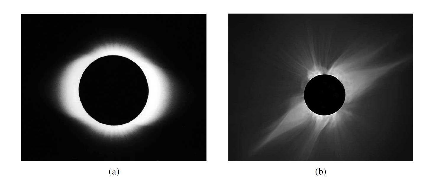
Fig. 6.10 (a) The quiet solar corona seen during a total solar eclipse in 1954. The shape of the corona is elongated along the Sun’s equator. (b) The active corona tends to have a very complex structure. This image of the July 11, 1991, eclipse is a composite of five photographs that was processed electronically. Image credit: Carroll & Ostlie (2007).

The corona is essentially transparent to most EM radiation (except long radio wavelengths) and is not in LTE. For gases that are not in LTE, a unique temperature is not strictly definable. Temperatures obtained by considering thermal motions, ionization levels, and radio emission do give consistent results. The presence of Fe XIV lines indicates temperatures in excess of \(2\times 10^6\) K, as do line widths produce by thermal Doppler broadening. Three structural components exist within the corona:

• K corona (from Kontinueirlich or “continuous”) produces continuous white light emission that results from photospheric radiation scattered by free electrons. Contributions from the K corona occur between \(1-2.3\:R_\odot\) from the Sun’s center. The spectral lines in the photosphere are essentially blended by the large Doppler shifts that are caused by the high thermal velocities of the electrons.

• F corona (for Fraunhofer) comes from the scattering of photospheric light by dust and grains beyond \(2.3\:R_\odot\). Dust grains are more massive (and slower) than electrons, so Doppler broadening is minimal and the Fraunhofer lines are still detectable. The F corona merges with the fait glow along the ecliptic that is a reflection of sunlight from interplanetary dust and is called zodiacal light.

• E corona is the source of the emission lines of highly ionized atoms throughout the corona. The E corona overlaps the K and F coronas. The temperatures are extremely high in the corona and the exponential term in the Saha equation encourages ionization. Very low number densities also encourage ionization since the potential for recombination is reduced.

The low number densities in the corona allow forbidden transitions to occur from atomic energy levels that are metastable (or temporarily stable). Electron do not readily make transitions from metastable states to lower energy states without assistance from another particle. Spontaneous forbidden transitions have a lifetime of ~1 s, where the allowed transitions have a life time of \(10^{-8}\) s. In high density gases, electrons escape from metastable states through collisions, but collisions are rare in the corona. Similar to the 21 cm hydrogen spin-flip transition, some electrons will make spontaneous transitions from metastable states to lower energy states given enough time.

The blackbody continuum from the Sun decreases following \(1/\lambda^4\) for sufficiently long wavelengths (Rayleigh-Jeans law) and thus, the amount of photospheric radio emission is negligible. The corona is a source of radio emission, where some of this emission arises from free-free transitions as electrons pass near ions. Due to these encounters, the change in energy of the electron determines the wavelength of the resulting photon through conservation of energy. Encounters in a higher density region (i.e., nearer to the Sun) result in shorter wavelength photons, where encounters in the chromosphere and lower corona (with much lower density) emit longer wavelength radiation \((1-20\:{\rm cm})\). Synchrotron radiation by relativistic electrons also contributes to the radio emission of the corona.

X-ray emissions from the photosphere are also rare, where the blackbody continuum decreases more rapidly (i.e., Wien approximation). Thus, any X-ray emission from the corona overwhelms the contribution from the photosphere due to its high temperature and low opacity at X-ray wavelengths. The corona contains a high degree of ionization for all the elements present, where the neutral atoms undergo a large number of transitions. Each element is capable of producing ans extensive emission spectrum.

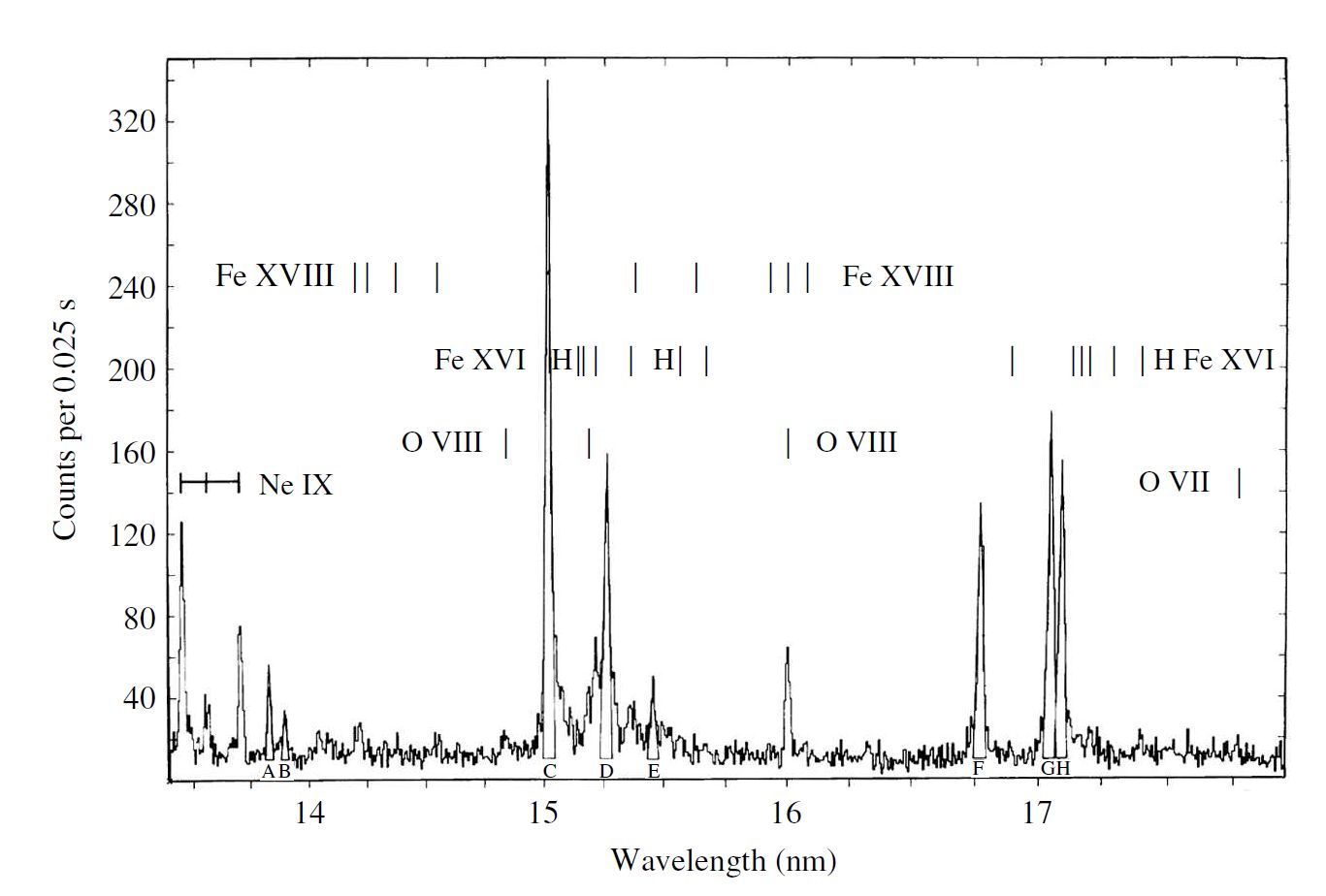
Fig. 6.11 A section of the X-ray emission spectrum of the solar corona. Image credit: Carroll & Ostlie (2007); figure adapted from Parkinson (1973).

6.2.4.1. Coronal Holes and the Solar Wind

Observations show that X-ray emission is non-uniform, where active (bright and hot) regions exist along with the coronal holes (darker and cooler regions). Within the coronal holes, localized bright spots (in X-ray wavelengths) can occur over a timescale of several hours. A weaker X-ray emission coming from the coronal holes is characteristic of the lower density and temperature of the region.

The existence of coronal holes is tied to the Sun’s magnetic field and the generation of a fast solar wind. The solar wind consists of a continuous stream of particles escaping from the Sun at speeds of approximately \(750\:{\rm km/s}\). A gusty, slow solar wind (speeds of about half the fast solar wind) is produced by streamers in the corona associated with closed magnetic fields.

The Sun’s magnetic field is similar to a dipole (on a global scale), although its value can differ significantly in localized regions and the field strength is typically \(\sim 10^{-4}\:{\rm T}\) near the surface (or a factor of few larger than Earth’s magnetic field at its surface). Coronal holes correspond to regions where the magnetic field lines are open, while the X-ray bright regions are associated with closed field lines. Closed field lines form loops that return to the Sun, while open field lines extend out to great distances.

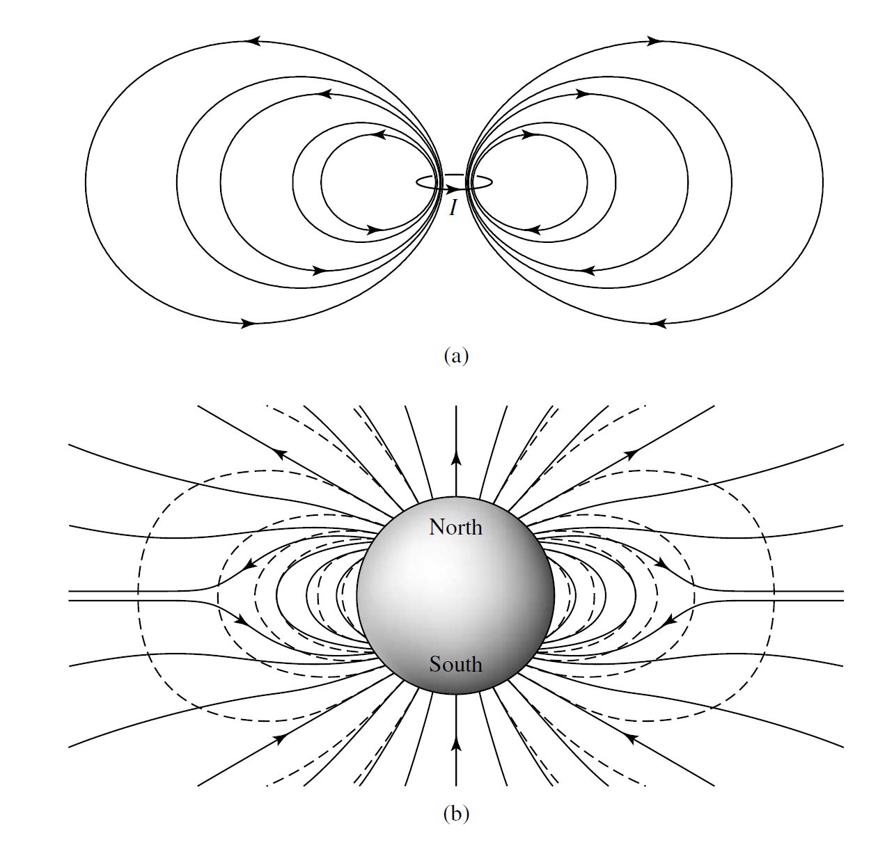
Fig. 6.12 (a) The characteristic dipole magnetic field of a current loop. (b) A generalized depiction of the global magnetic field of the Sun. The dashed lines show the field of a perfect magnetic dipole. Image credit: Carroll & Ostlie (2007).

For charged particles moving in an external magnetic field, the Lorentz force equation applies

(6.2)\[\begin{align} \mathbf{F} = q(\mathbf{E} + \mathbf{v} \times \mathbf{B}), \end{align}\]

which describes the force \(\mathbf{F}\) exerted on a charged particle \(q\) with a velocity \(\mathbf{v}\) in an electric field \(\mathbf{E}\) and magnetic field \(\mathbf{B}\). Due to the vector cross product, the force is always mutually perpendicular to both the direction of the velocity and magnetic field (i.e., right-hand rule). Assuming that the electric field is negligible \((E \ll vB\sin\theta)\), charged particles are forced to spiral around the magnetic field lines and cannot actually ross them except by collisions. Closed magnetic field lines tend to trap charged particles, while open field lines allow the particles to travel away from the Sun. Thus, the solar wind originates from the coronal holes (or regions of open magnetic field lines). The bright regions in X-ray observations are due to the higher densities of charged particles (electrons and ions) that are trapped in large and small magnetic field loops. A similar mechanism of trapping charged particles in magnetic fields occurs on the Earth through the auroras (aurora borealis (northern lights) and aurora australis (southern lights)) and the Van Allen radiation belts.

Note

The existence of ongoing mass loss from the Sun (i.e., solar wind) was deduced from comet tails, where a radiation pressure coming from the Sun pushes back the dust tail.

The Ulysses spacecraft was placed on an inclined, heliocentric orbit and was still able to detect the solar wind. At 1 AU, the solar wind velocity ranges from \(200-750\:{\rm km/s}\) with a typical density of \(7\times10^6\:{\rm ions/m^3}\), and characteristic kinetic temperatures of \(10^4-10^5\) K for protons and electrons.

Exercise 6.1

What is the mass loss rate of the Sun?

From the information above, we know the approximate number density of particles at 1 AU and assuming that the mass loss rate is spherically symmetric, then the mass loss is simply the mass density \(\rho\) that can cross a spherical shell of a radius \(r\) in a time \(t\),

\[ dM = \rho dV = (nm_H)(Av\:dt) = (nm_H)(4\pi r^2\:v\:dt), \]

where the mass density depends on the number density \(n\) and particle mass \(m_H\) (assumed to be hydrogen). The mass loss rate can be obtained by dividing both sides to get

(6.3)\[\frac{dM}{dt} = 4\pi r^2\:nm_H\:v. \]

Note

By convention, stellar mass loss rates are given in solar masses per year and the rate is symbolized as \(\dot{M}\equiv {dM/dt}\).

import numpy as np 
from scipy.constants import au, m_p

def Mass_loss(r,n,v):
    #r = radius of the spherical shell; in m
    #n = number density of ions; in ions/m^3
    #v = speed of the ions; in m/s
    Mdot = (4*np.pi*r**2)*(n*m_p)*v
    return Mdot*(365.25*86400)/M_sun #mass loss rate; converted into M_sun/yr

M_sun = 1.989e30 #solar mass in kg
v_H = 0.5*(750 + 200)*1000 #average particle velocity; converted to m/s
r = 1*au #radius of shell; converted to m
n = 7e6 #number density of ions; ions/cm^3

Sun_loss = Mass_loss(r,n,v_H)
print("The mass loss rate of the Sun is approximately %1.3e M_sun/yr." % Sun_loss)
print("The entire Sun's mass would be depleted in %1.3e yr." % (1/Sun_loss))

The mass loss rate of the Sun is approximately 2.482e-14 M_sun/yr.
The entire Sun's mass would be depleted in 4.030e+13 yr.

It would require more than \(10^{13}\) yr (or \(10^4\) Gyr) before the entire mass of the Sun is dissipated and so the effect of the present-day solar wind negligible compared to the evolution of the Sun’s interior.

6.2.4.2. The Parker Wind Model

Since the corona is very hot and has a high thermal conductivity, it can referred to as a plasma. The ability of a plasma to conduct heat implies that the corona is almost isothermal. In 1958, Eugene Parker developed an approximately isothermal model of the solar wind.

We begin by considering the corona to be in hydrostatic equilibrium, which means that the outward pressure is balanced by the inward pull of gravity. If the mass of the corona is insignificant compared to the total mass of the Sun, then the mass enclosed at a given radius of the corona \(M_r\) is approximately equal to \(M_\odot\) (i.e., \(M_r \approx M_\odot\)) and the equation for the hydrostatic equilibrium becomes

(6.4)\[\frac{dP}{dr} = -\frac{G M_\odot \rho}{r^2}. \]

For simplicity, we assume that the gas is completely ionized hydrogen so that the number density of protons is given by

\[ n \approx \frac{\rho}{m_p}. \]

Then, from the ideal gas law we can write the pressure as

\[ P = 2nkT, \]

where \(\mu = 1/2\) for ionized hydrogen (from statistical mechanics) and \(m_H\approx m_p\). Substituting into Eqn. (6.4) and the hydrostatic equilibrium equation becomes

(6.5)\[\frac{d}{dr}(2nkT) = - \frac{GM_\odot nm_p}{r^2}.\]

For an isothermal gas, Eqn. (6.5) can be integrated directly and solved for the number density as a function of radius \(n(r)\) or

(6.6)\[\begin{align} n(r) = n_o e^{-\lambda (1-r_o/r)}, \end{align}\]

where

\[ \lambda \equiv \frac{GM_\odot m_p}{2kTr_o} \]

and there is some number density \(n_o\) at a radius \(r_o\).

Note

The value of \(\lambda\) is approximately the rato of a proton’s gravitational potential energy \((GM_\odot m_p/r_o)\) and its thermal kinetic energy \((2kT)\).

The pressure structure is related to the number density (via the ideal gas law) and can be written as

\[ P(r) = P_o e^{-\lambda (1-r_o/r)}, \]

where \(P_o = 2n_o kT\).

An immediate consequence is that the pressure does not approach zero as \(r\) goes to infinity. Typical values of the inner corona are: \(T = 1.5 \times 10^6\) K and \(n_o = 3 \times 10^{13}\:{\rm m^{-3}}\) at \(r_o = 1.4\:R_\odot\). Then,

\[ \lambda = \frac{(6.67 \times 10^{-11}\:{\rm m^3/kg/s^2})(1.989 \times 10^{30}\:{\rm kg})( 1.67\times 10^{-26}\:{\rm kg})}{2 (1.381 \times 10^{-23}\:{\rm m^2 kg/s^2/K})(1.5\times 10^6\:{\rm K})(9.740 \times 10^8\:{\rm m})} = \mathbf{5.5}\]

\[ n(\infty) = (3 \times 10^{13}\:{\rm m^{-3}})/e^{\lambda} = \mathbf{1.2 \times 10^{11}\:{\rm m^{-3}}}\]

and

\[ P(\infty) = 2(1.381 \times 10^{-23}\:{\rm m^2 kg/s^2/K})(1.5\times 10^6 \:{\rm K})(3 \times 10^{13}\:{\rm m^{-3}})/e^{\lambda} = \mathbf{5 \times 10^{-6}\:{\rm N/m^2}}. \]

from scipy.constants import k, m_p, G
import numpy as np

M_odot = 1.989e30 #Solar mass in kg
R_odot = 6.957e8 #Solar radius in m

T = 1.5e6 #temperature in K
n_o = 3e13 #number density in m^{-3}

lam = (G*M_odot*m_p)/(2*k*T*(1.4*R_odot))
n_infty = n_o*np.exp(-lam)
P_infty = 2*n_o*k*T*np.exp(-lam)

print("The value of lambda is %1.1f." % lam)
print("The number density at infinity is %1.1e." % n_infty)
print("The pressure at infinity is %1.0e." % P_infty)

The value of lambda is 5.5.
The number density at infinity is 1.2e+11.
The pressure at infinity is 5e-06.

With the exception of localized clouds, the actual densities and pressures of interstellar dust and gas are much lower that those just derived.

The assumption that the corona is approximately isothermal is not completely valid, but it is roughly consistent with observations. Apparently, the assumption that the corona is in hydrostatic equilibrium is wrong. Since \(P(\infty)\) greatly exceeds the pressures in interstellar space, material must be expanding outward from the Sun, implying the existence of the solar wind.

6.2.5. The Hydrodynamic Nature of the Upper Solar Atmosphere

To develop a better understanding of the solar atmosphere’s structure, the approximation of hydrostatic equilibrium must be replaced by a set of hydrodynamic equations that describe the flow. In particular, we can write the acceleration as

\[ \frac{d^2 r}{dt^2} = \frac{dv}{dt} = \frac{dv}{dr}\frac{dr}{dt} = v\frac{dv}{dr}, \]

using the chain rule and add a term to Eqn. {eq}`Pressure_grad’ to get

(6.7)\[\begin{align} \rho v\frac{dv}{dr} = -\frac{dP}{dr} - \frac{GM_r \rho}{r^2}, \end{align}\]

where \(v\) is the velocity of the flow. From fluid dynamics, there is also a conservation of mass flow across a boundary and is written as

\[ 4\pi r^2 \rho v = {\rm constant}, \]

which is similar to Eqn. (6.3) that was used to estimate the Sun’s mass loss rate. Since the mass flow is conserved, we immediately get

\[ \frac{d(\rho vr^2)}{dr} = 0. \]

In the convection zone there is a motion of the hot gas rising and the return flow of the cool gas sinking, which sets up longitudinal (pressure) waves that propagate outward through the photosphere and into the chromosphere. The outward flux of wave energy \(F_E\) is given by

(6.8)\[\begin{align} F_E = \frac{1}{2}\rho v_w^2 v_s, \end{align}\]

which depends on the local sound speed \(v_s\) and the velocity amplitude \(v_w\) of particles that oscillate relative to their equilibrium positions. The sound speed is given by

\[ v_s = \sqrt{\frac{K}{\rho}} = \sqrt{\frac{\gamma P}{\rho}}, \]

which depends on gas density \(\rho\) and the bulk modulus \(K\) (or the adiabatic index \(\gamma\) and gas pressure \(P\)). From the ideal gas law, the pressure can be written as

\[ P = \frac{\rho k T}{\mu m_H} \]

and the sound speed can be written as

\[ v_s = \sqrt{\frac{\gamma k T}{\mu m_H}}. \]

For a fixed \(\gamma\) and \(\mu\), \(v_s \propto \sqrt{T}\).

A wave that begins at the top of the convection zone will have a wave oscillation amplitude less than the sound speed (\(v_w<v_s\)). However, the gas density decreases with altitude dropping by a factor of \(10^4\) in approximately 1000 km. The wave oscillation amplitude \(v_w\) must significantly increase, assuming that \(4\pi r^2 F_E \approx {\rm constant}\) (i.e., very little mechanical energy loss) and the sound speed \(v_s\) remains essentially unchanged. This increase in wave oscillation amplitude makes the motion become supersonic (\(v_w>v_s\)) as particles travel faster than the sound speed. The wave develops into a shock wave much like the energy wave that triggers a tsunami.

A shock wave is characterized by a steep density change over a short distance, which is called the shock front. A shock moving through a gas produces a great deal of heat via collision, which leaves the gas in its wake highly ionized. The heating comes at the expense of mechanical energy of the shock and thus, the shock quickly dissipates. The gas in the chromosphere and above is effectively heated by the mass motions created in the convection zone.

6.2.6. Magnetohydrodynamics and Alfvén Waves

The photosphere is also influenced by the Sun’s magnetic field in which our discussion has yet failed to take into account. The temperature structure of the outer solar atmosphere is expected to result from the presence of the magnetic field. Magnetohydrodynamics (or MHD) is the study of interactions between magnetic fields and plasmas. A complete solution to the MHD equations applied to the Sun’s outer atmosphere does not yet exist. but, there are some useful aspects to the partial solutions.

A second kind of wave motion can be generated by the presence of a magnetic field, which are transverse waves that propagate along a magnetic field line. These waves are a consequence of the restoring force associated with the magnetic field lines. Recall that a magnetic field requires energy (i.e., no magnetic monopole) through moving charges or currents and the energy can be described as begin stored within the magnetic field itself as a magnetic field energy density \(u_m\). The value of the magnetic energy density is given by

(6.9)\[\begin{align} u_m = \frac{B^2}{2\mu_o}, \end{align}\]

which depends on the permeability of free space \(\mu_o = 4\pi \times 10^{-7}\:{\rm Tm/A}\). Recall that \(1\:{\rm T} = 1 {\rm \frac{N}{A\cdot m}}\).

The density of magnetic field lines increases if a plasma (containing a number of magnetic field lines) is compressed in a direction perpendicular to the lines. But the density of lines is proportional the strength of the magnetic field itself and the energy density increases during the compression. A change in volume (i.e., compression) of the plasma leads to work being done \((W=\int P dV)\) and this implies the existence of a magnetic pressure, which is equal to the magnetic energy density,

(6.10)\[\begin{align} u_m = P_m = \frac{B^2}{2\mu_o}. \end{align}\]

The magnetic pressure gradient acts to compensate for an increase in the magnetic pressure in the direction of the magnetic field lines with an decrease in pressure in the opposite direction. The pressure change restores the field line density to its original value. This process is analogous to how the tension restores a string after it is plucked and a wave propagates along the string. This transverse MHD wave is called an Alfvén wave.

Note

Hannes Olof Gösta Alfvén (1908-1995) was awarded the Nobel Prize in 1970 for his fundamental studies in MHD and thus, Alfvén waves are named after him.

The propagation speed of an Alfvén wave can be estimated using an analogy to the adiabatic sound speed \(v_s\), where \(\gamma \approx 1\) as:

\[ v_m \sim \sqrt{\frac{P_m}{\rho}} = \frac{B}{\sqrt{2\mu_o \rho}}, \]

and a more careful treatment gives

(6.11)\[\begin{align} v_m = \frac{B}{\sqrt{\mu_o \rho}}. \end{align}\]

Exercise 6.2

How does the sound speed compare to the Alfvén speed in the solar photosphere?

The gas pressure at the top of the photosphere is roughly \(140\:{\rm N/m^2}\) with a density of \(4.9\times 10^{-6}\:{\rm kg/m^3}\). Assuming an ideal monatomic gas (\(\gamma = 5/3\)), the sound speed is

\[ v_s = \sqrt{\frac{(5/3)(140\:{\rm N/m^2})}{4.9\times \times 10^{-6}\:{\rm kg/m^3}}} \simeq 7000 \:{\rm m/s}. \]

A typical surface magnetic field strength is \(2\times 10^{-4}\:{\rm T}\), then the magnetic pressure is

\[ P_m = \frac{(2\times 10^{-4}\:{\rm T})^2}{2(4\pi \times 10^{-7}\:{\rm T m/A})} \simeq 0.02\:{\rm N/m^2}. \]

Then the Alfvén speed is

\[ v_m = \frac{2\times 10^{-4}\:{\rm T}}{\sqrt{(4\pi \times 10^{-7}\:{\rm T m/A})(4.9\times \times 10^{-6}\:{\rm kg/m^3})}} = 81\:{\rm m/s}. \]

The magnetic pressure may generally be neglected in photospheric hydrostatic considerations because it is smaller than the gas pressure by roughly four orders of magnitude (i.e., \(P_{\rm photo}/P_m\)). However, much larger magnetic field strengths can exist in localized regions on the Sun’s surface.

Note

Example 2.2 in the textbook (Carroll and Ostlie 2007) has a typographical error, where the Alfvén speed should be \(v_m \simeq 100\) m/s.

import numpy as np
from scipy.constants import mu_0

P_photo = 140 #gas pressure at the top of the photosphere in N/m^2
gamma = 5./3. #monatomic adiabatic gas constant
rho_photo = 4.9e-6 #gas density as the top of the photosphere in kg/m^3
B_photo = 2e-4 #magnetic field strength at the top of the photosphere in T

v_s = np.sqrt(gamma*P_photo/rho_photo)
P_m = B_photo**2/(2*mu_0)
v_m = B_photo/np.sqrt(mu_0*rho_photo)

print("The sound speed is approximately %4d m/s." % np.round(v_s,-3))
print("The magnetic pressure is %1.3f N/m^2." % np.round(P_m,2))
print("The Alfven speed is %2d m/s." % np.round(v_m,0))

The sound speed is approximately 7000 m/s.
The magnetic pressure is 0.020 N/m^2.
The Alfven speed is 81 m/s.

Alfvén waves transport energy outwards, since they can propagate along magnetic field lines. From Maxwell’s equations, a time-varying magnetic field induces electrical currents in a highly conductive plasma and thus, some resistive Joule heating will occur causing the temperature to rise. MHD wave can also contribute to the temperature structure of the upper solar atmosphere.

The Sun’s rotation drags the open magnetic field lines along through interplanetary space. The solar wind is forced to move with the field lines and a torque is produced that actually slows the Sun’s rotation. The differential rotation present in the photosphere is not manifested in the corona, which is interesting because the magnetic field influences the structure of the corona but not through its rotation.

6.3. The Solar Cycle

6.3.1. Sunspots

It was Galileo who made the first telescopic observations of sunspots. Even though sunspots are occasionally visible with the naked eye, making such observations is strongly discouraged due to the potential for eye damage. Newton temporarily blinded himself by trying to look at the Sun using a mirror, though not to observe sunspots. Reliable observations over the past 200 years show the number of sunspots and the average latitude of sunspot formation is approximately periodic with an 11-year cycle. A plot of the sunspot location over time is known as the butterfly diagram. Individual sunspots are short-lived (surviving no more than an month or so). A sunspot remains at a constant latitude over its lifetime, while successive sunspots form at progressively lower latitudes. New cycles of sunspots occur near \(\pm 40^\circ\) relative to the equator.

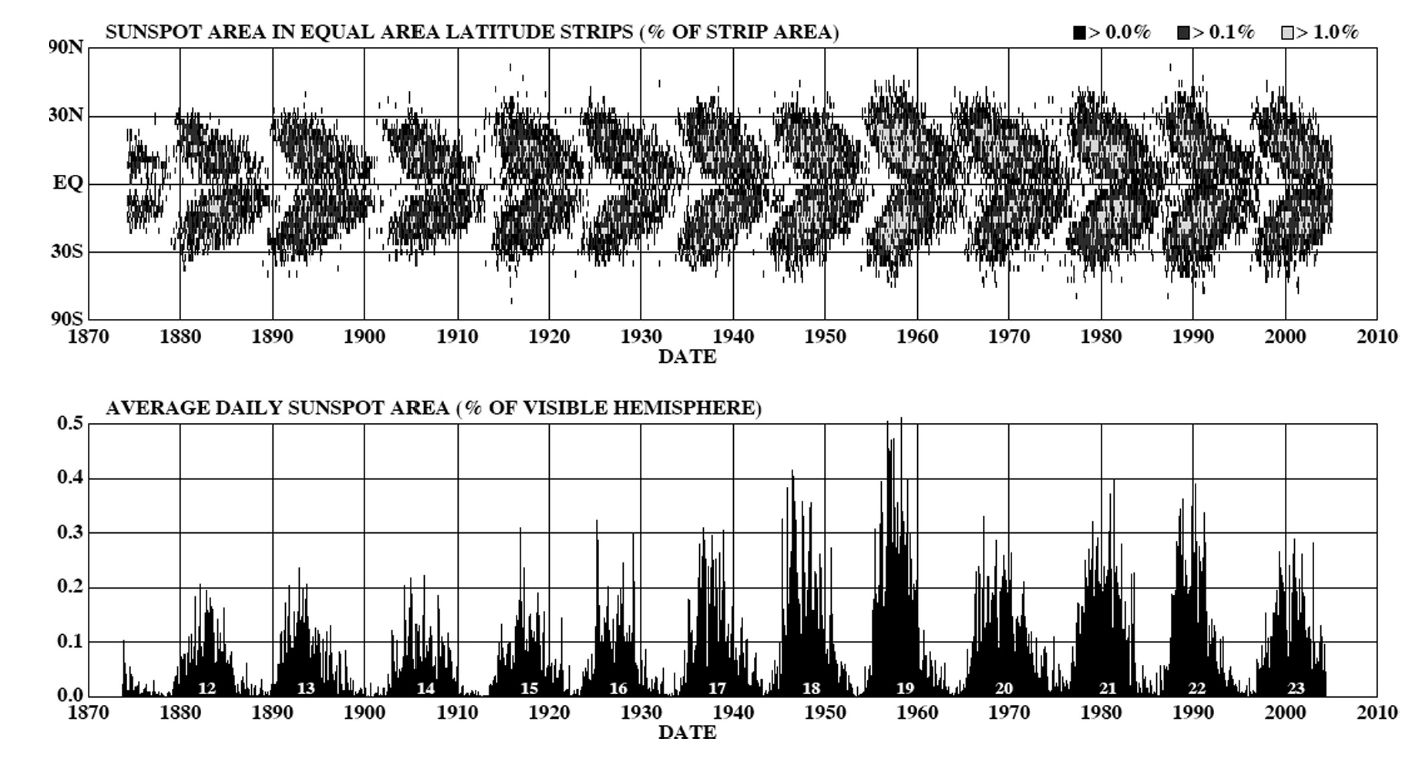
Fig. 6.13 The upper figure depicts the butterfly diagram, showing sunspot latitudes with time. The lower figure shows the percentage of the Sun’s surface covered by sunspots as a function of time. Image credit: Carroll & Ostlie (2007).

A key to understanding sunspots lies in their strong magnetic fields. The darkest part of a sunspot is called the umbra and can be up to 30,000 km in diameter (\(\sim2.5\times\) Earth’s diameter). The umbra is usually surrounded by the penumbra, whose appearance indicates the presence of magnetic field lines. The magnetic fields can be measured through the Zeeman effect (i.e., splitting of spectral lines due to an external magnetic field), where such measurements indicate the strength and polarity of the magnetic field. Magnetic field strengths \(\gtrsim 0.1\) T have been measured in the centers of umbral regions and the field strength decreases across the penumbral regions.

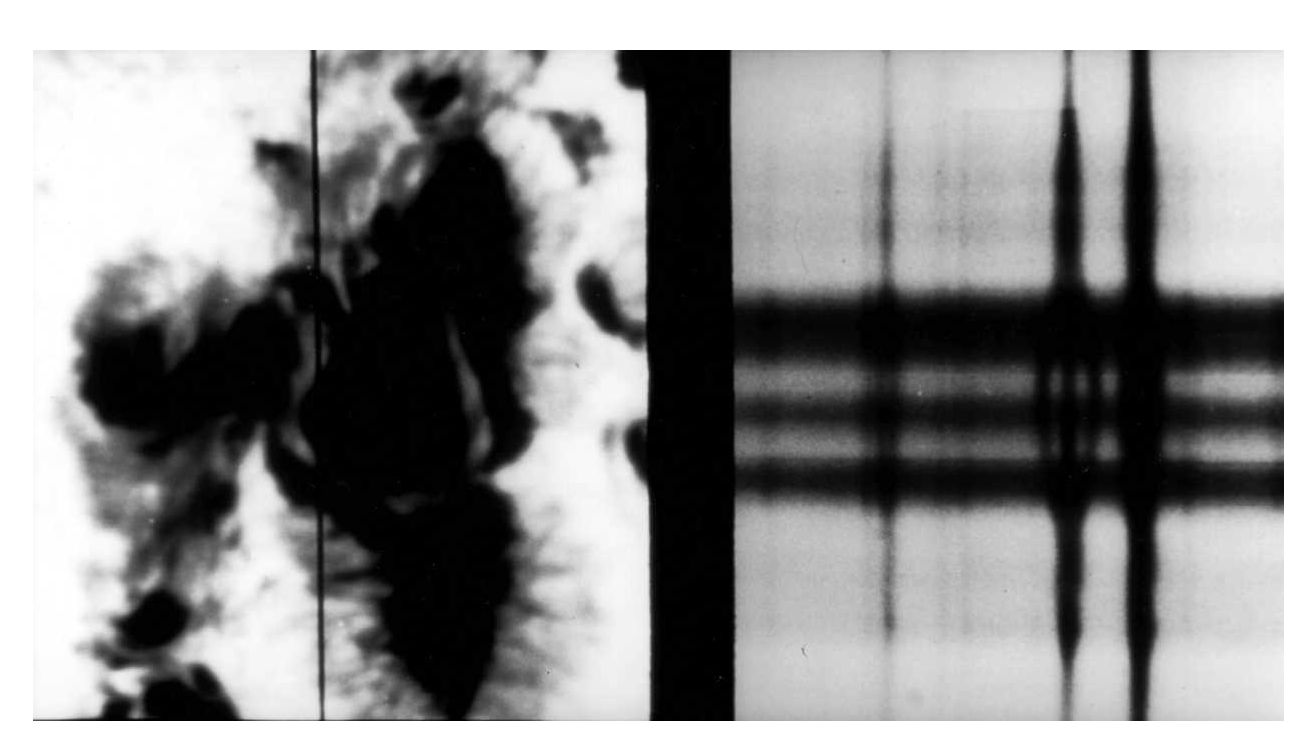
Fig. 6.14 The Zeeman splitting of the Fe 525.02-nm spectral line due to the presence of a strong magnetic field in a sunspot. Image credit: Carroll & Ostlie (2007).

Sunspots typically occur in groups, where a dominant sunspot leads in the direction of rotation and the remaining sunspots follow the leader. During a cycle, the lead sunspot pair at symmetric latitudes (relative to the equator) will have opposite polarity, while the trailing sunspot pairs will have the opposite polarity. During each successive 11-year sunspot cycle the polarities will be reversed. Accompanying this local polarity reversal is a global polarity reversal of the Sun’s entire dipole. Polarity reversals of the Sun occur on a 22-year cycle.

The dark appearance of the umbra is caused by their significantly lower temperatures (~3900 K) relative to the effective temperature (5777 K). The luminosity difference is proportional to the temperature ratios raised to the fourth power, where a sunspot can be (5777/3900)\(^4\) = 4.8 times fainter than the surrounding photosphere. Each sunspot has a lifetime of about a month and thus luminosity variations also occur on a timescale of months. Although the Sun’s luminosity can experience a luminosity variation over a much longer timescale. For example, very few sunspots were observed from \(1645-1715\), which corresponds to the Maunder minimum.

With lower temperatures in sunspots, the gas pressure is also lower than the surrounding material and we would expect that gravity would cause the gas within a sunspot to sink. But this is not observed, where the extra magnetic pressure supports the sunspot and keeps it from sinking.

Plages (from the French word for beach) are chromospheric regions of bright \({\rm H\alpha}\) emission located near active sunspots. They usually appear before the sunspots and disappear after the sunspots vanish. Plages have higher densities that the surrounding gas and are products of magnetic fields .

6.3.2. Solar Flares

Solar flares are eruptive events that release between \(10^{17}-10^{25}\) J of energy over a range of time intervals (millisecond to more than an hour). A large flare can reach 100,000 km in length. During an eruption, the \({\rm H \alpha}\) line appears locally in emission rather than in absorption, implying that photon production occurs above much of the absorbing material. Other types of EM radiation are produced that can range from nonthermal radio (~1 km) waves due to synchrotron radiation to hard (very short wavelength) X- and gamma-ray emission lines.

Charge particles are also ejected outward at high speeds becoming solar cosmic rays when they escape into interplanetary space. The ejected charged particles (mostly protons and helium nuclei) can reach Earth in 30 min, disrupting communications and pose a threat to astronauts. Shock waves can occasionally propagate several AU before dissipating.

What powers a solar flare?

The answer lies in the location of the flare eruption. Flares develop in regions of great magnetic field intensity (e.g., sunspot groups). The creation of magnetic fields results in energy storage in those magnetic fields. A flare might develop when the stored energy is quickly released. The details of the energy conversion are still a matter of active research.

A model of a solar flare shows the general mechanism involves reconnection of magnetic field lines. A disturbance in the magnetic field loops causes the creation of sheet of current in the highly conducting plasma (via Lenz’s law). The Joule heating from the resistance in the plasma causes temperatures to reach \(10^7\) K. Particles accelerated away from a reconnection point (and away from the Sun) can escape the Sun entirely to become solar cosmic rays. Radio, soft X-rays, and \({\rm H\alpha}\) emission can all occur as a result of the reconnection.

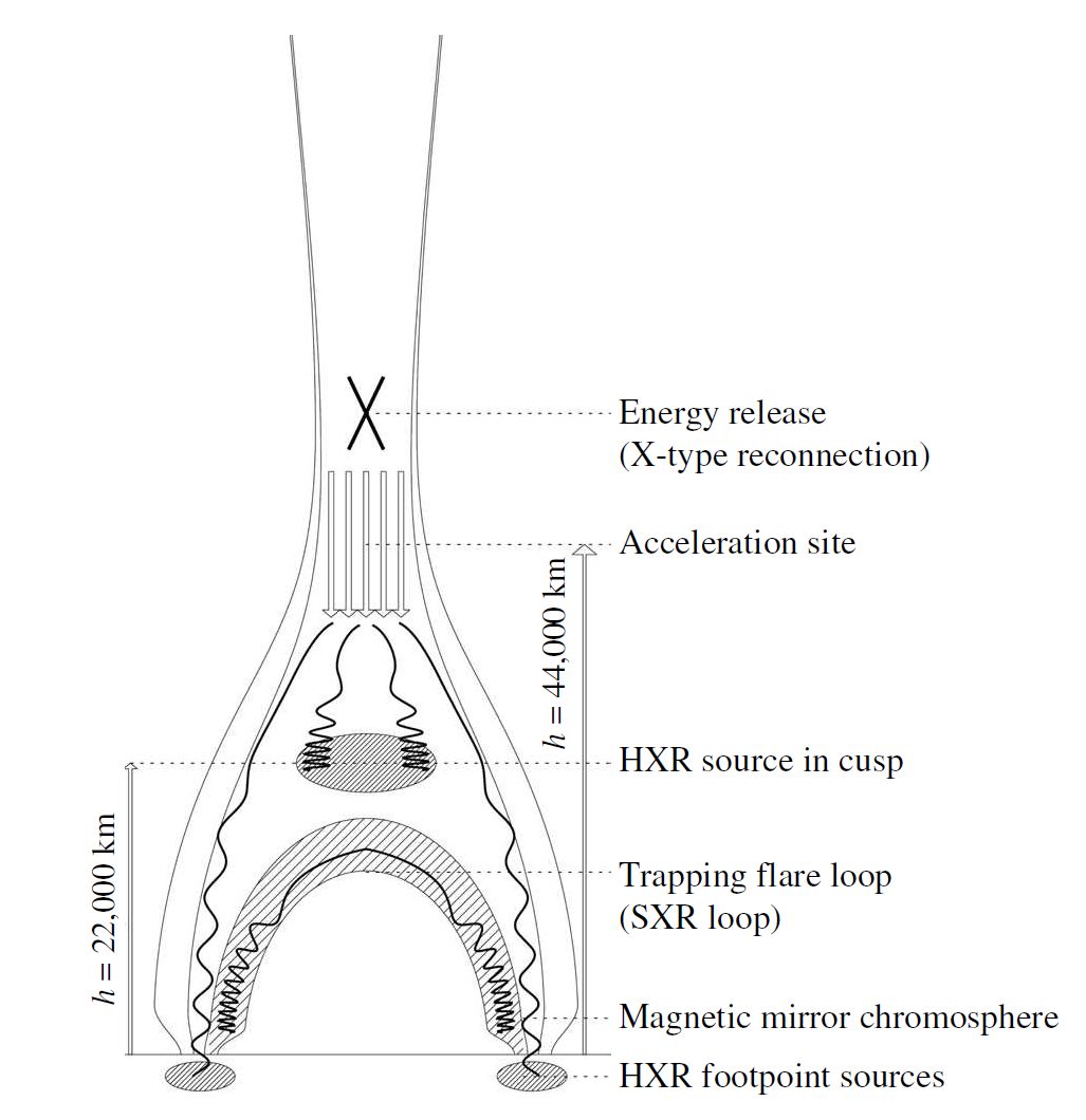
Fig. 6.15 A model of the January 13, 1992, Masuda solar flare. Note the two hard X-ray (HXR) footpoint sources associated with \({\rm H \alpha}\) flare ribbons. Electrons are accelerated downward along the magnetic field lines until they collide with the chromosphere. Image credit: Carroll & Ostlie (2007); figure adapted from Aschwanden et al. (1996).

High-energy particles accelerated toward the chromosphere produce hard X-rays and gamma rays due to surface nuclear reactions. Spallation reactions break heavier nuclei into lighter nuclei and are associate with solar flares. Some example reactions are

\[ ^1_1{\rm H} + ^{16}_8{\rm O} \rightarrow ^{12}_6{\rm C^*} + ^{4}_2{\rm He} + ^1_1{\rm H}, \]

where \(C^*\) represents a carbon nucleus in an excited state, followed by a de-excitation reaction

\[ ^{12}_6{\rm C^*} \rightarrow ^{12}_6{\rm C} + \gamma, \]

that produces a 4.438 MeV photon, or

\[ ^1_1{\rm H} + ^{20}_{10}{\rm Ne} \rightarrow ^{16}_8{\rm O^*} + ^{4}_2{\rm He} + ^1_1{\rm H}, \]

followed by a de-excitation reaction

\[ ^{16}_8{\rm O^*} \rightarrow ^{16}_8{\rm O} + \gamma, \]

that produces a 6.129 Mev photon. Flares can also produce electron-positron annihilation on the Sun’s surface (resulting in 0.511 MeV photons) and deuterium by

\[ ^1_1{\rm H} + {\rm n} \rightarrow ^2_1{\rm H^*} \rightarrow ^2_1{\rm H} + \gamma, \]

with a 2.223 MeV photon.

6.3.3. Solar Prominences & Coronal Mass Ejections

A solar prominence is a large plasma and magnetic field structure that extends outwards from the Sun. Quiescent prominences (or curtains of ionized gas) reach into the corona and can remain stable for weeks (or months). An active region collects material along its magnetic field lines, which results in a cooler, denser gas compared to the surrounding corona. This causes the gas to “rain” back down into the chromosphere. An active (or eruptive) prominence may exist for only a few hours, where it disappears due to instabilities in the magnetic field lines that cause the prominence to lift away from the Sun. This is similar to the production of flares, but the eruptive material is mainly gas ejected (i.e., coronal mass ejection or CMEs) from the Sun instead of EM radiation.

The solar corona can extend from a few solar radii up to \(30\:{\rm R_\odot}\) and can average about one CME occurs per day over the 11-year sunspot cycle. When the Sun is more active, this rate can increase to 3.5 CMEs per day. At a solar minimum, the rate of CMEs decreases substantially to one event every five days. During a CME event between \(5\times 10^{12} - 5\times 10^{13}\) kg of material may be ejected from the Sun traveling at speeds ranging from \(400-1000\) km/s. CMEs appear to be associated with prominences 70% of the time and flares 30% of the time. CMEs are like magnetic bubbles that lift material of the Sun’s surface after a reconnection event and can carry a significant portion of the corona with it.

6.3.4. The Magnetic Dynamo Theory

A magnetic dynamo was first proposed by Horace Babcock in 1961, which describes many components of the solar cycle. Despite its general success, the models doesn’t provide a complete picture. Any complete picture will require:

• full treatment of the MHD equations in the solar environment,

• differing rotation rates with latitude and depth of the Sun,

• convection,

• solar oscillations,

• heating of the upper atmosphere, and

• mass loss.

Not all of these processes are equally important, but a complete model should indicate the degree to which each process contributes.

At the beginning of a cycle, the magnetic field lines are “frozen” into the gas, but the differential rotation of the Sun drags the lines along. This converts a poloidal field (i.e., magnetic dipole) into a field with a toroidal component that wraps around the Sun. The turbulent convection zone can twist the magnetic field lines and create magnetic ropes (i.e., regions of intense magnetic field due higher density of lines). The magnetic pressure forces the ropes to rise to the surface as sunspot groups. The polarity of the sunspots comes from the direction of magnetic field along the ropes.

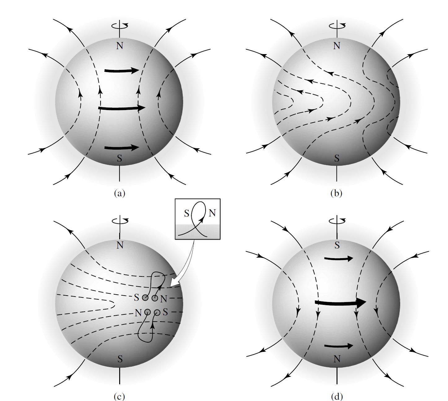
Fig. 6.16 The magnetic dynamo model of the solar cycle. (a) The solar magnetic field is initially a poloidal field. (b) Differential rotation drags the “frozen-in” magnetic field lines around the Sun. (c) Turbulent convection twists the field lines into magnetic ropes. (d) As the cycle progresses, successive sunspot groups migrate toward the equator where magnetic field reconnection reestablishes the poloidal field, but with the original polarity reversed. Image credit: Carroll & Ostlie (2007).

The twisting begins at higher latitudes during a sunspot minimum, then differential rotation drags the field lines and convective ties them into knots, and more sunspots appear at intermediate latitudes leading to a sunspot maximum. One might expect the greatest amount of twisting to occur at the equator, but sunspots near the equator tend to cancel each other out due to the polarity of the leading spots being opposed. The cancellation of magnetic fields near the equator causes the poloidal field to be re-established, but with a reversal of polarity.

6.4. Homework

Problem 1

Using the Saha equation, calculate the ratio of the number of \(H^−\) ions to neutral hydrogen atoms in the Sun’s photosphere. Take the temperature of the gas to be the effective temperature, and assume that the electron pressure is \(1.5\:{\rm N/m^2}\). *Note that the Pauli exclusion principle requires that only one state can exist for the ion because its two electrons must have opposite spins.

Problem 2

The Paschen series of hydrogen (\(n = 3\)) can contribute to the visible continuum for the Sun since the series limit occurs at 820.8 nm. However, it is the contribution from the \(H^−\) ion that dominates the formation of the continuum. Using the results of Problem 1 above, along with the Boltzmann equation, estimate the ratio of the number of \(H^−\) ions to hydrogen atoms in the \(n = 3\) state.

Problem 3

The gas pressure at the base of the photosphere is approximately \(2 \times 10^4\:{\rm N/m^2}\) and the mass density is \(3.2 \times 10^{-4}\:{\rm kg/m^3}\).

(a) Estimate the sound speed at the base of the photosphere.

(b) Compare your answer with the values at the top of the photosphere and averaged throughout the Sun.

Problem 4

Assuming that an average of one coronal mass ejection (CME) occurs per day and that a typical CME ejects \(10^{13}\) kg of material, estimate the annual mass loss from CMEs and compare your answer with the annual mass loss from the solar wind. Express your answer as a percentage of CME mass loss to solar wind mass loss.

Problem 5

Assume that the velocity of a CME directed toward Earth is 400 km/s and the mass of the CME is \(10^{13}\) kg.

(a) Estimate the kinetic energy contained in the CME and compare your answer to the energy released in a large flare. Express your answer as a percentage of the energy of the flare.

(b) Estimate the transit time for the CME to reach Earth.

(c)* Briefly explain how astronomers are able to “predict” the occurrence of aurorae in advance of magnetic storms on Earth.

Problem 6

Assume that the magnetic field strength inside a sunspot is 0.3 T.

(a) Calculate the frequency shift produced by the normal Zeeman effect in the center of a sunspot.

(b) By what fraction would the wavelength of one component of the 630.25 nm Fe I spectral line as a consequence of the magnetic field inside a sunspot.