14. Fluid Mechanics

May 06, 2026 | 12877 words | 64 min read

14.1. Fluids, Density, and Pressure

This audio is AI-generated.

14.1.1. Characteristics of Solids and Fluids

Solids are rigid, have specific shapes, and occupy definite volumes. The atoms (or molecules) in a solid are in close proximity to each other, where there is a significant force between the molecules. Solids will take a form that is determined by the forces between the molecules. True solids are compressible, where it usually takes a large force to change the shape of a solid.

• The force between the molecules can allow them to organize into a lattice.

• The structure of the 3D lattice is represented as molecules connected by rigid bonds (modeled as stiff springs), which allow limited freedom of movement.

• Even a large force produces only small displacements in the atoms (or molecules) of the lattice, and the solid maintains its shape. Solids also resist shearing forces (see Section 12.3).

Liquids and gases are both described as fluids of varying viscosity because they yield to shearing forces, whereas solids resist them. Like solids, the molecules in a liquid are bonded to neighboring molecules, but there are fewer (and weaker) bonds.

• The molecules in a liquid are not locked in place and can move with respect to each other.

• The distance between molecules is similar to the distances in a solid. Liquids have definite volumes, but the shape of a liquid can change depending on the shape of its container.

• Gases are not bonded to neighboring atoms and can have large separations between molecules.

• Gases have neither specific shapes nor definite volumes, where their molecules move to fill the container.

Liquids deform easily when stressed and do not spring back to their original shape once a force is removed. This occurs because the atoms (or molecules) are free to slide about and change neighbors. Liquids flow with the molecules held together by looser mutual attraction. When a liquid is placed in a container, it remains in the container (given the appropriate temperature and atmospheric pressure). Because the atoms are closely packed liquids resist compression, where an extremely large force is necessary to change the volume of a liquid.

Atoms in gases are separated by large distances and the forces between atoms in a gas are very weak, except when the atoms collide with one another. This makes gases relatively easy to compress and allows them to flow like a fluid. When placed in an open container, gases will escape.

Given the right conditions gases and fluids behave in similar ways, where it is common to drop the distinction and consider them both as fluids. There exists another phase of matter called a plasma, which exists at high temperatures, which is characterized by being composed of ions rather than neutral atoms. Plasma has different properties, which requires a detailed description of electrical charges and forces.

14.1.2. Density

Suppose a block of brass and a block of wood have exactly the same mass. If both blocks are dropped in a tank of water, why does the wood float and the brass sink? This occurs because the brass has a greater density than water.

Density is an important characteristic of substances because it is crucial in determining whether an object sinks or floats in a fluid.

Density

The average density of a substance or object is defined as its mass per unit volume,

(14.1)\[\begin{align} \rho = \frac{m}{V}, \end{align}\]

where \(\rho\) (\rho) is the symbol for density, \(m\) is the mass, and \(V\) is the volume.

The SI unit for density is \(\rm kg/m^3\), where Table 14.1. Many materials are more easily measured using lower masses and/or volume which makes the \(\rm cgs\) units system useful. The \(\rm cgs\) density is the gram per cubic centimeter or per milliliter \(\rm mL\), where

\[ 1\ {\rm g/cm^3} = 1\ {\rm g/mL} = 1000\ {\rm kg/m^3}.\]

The metric system was originally devised so that water would have a density of \(1\ {\rm g/cm^3}\), thus the basic mass unit (the kilogram) was first devised to be the mass of \(1\ {\rm L} = 1000\ {\rm mL}\) volume of water.

Table 14.1 Densities of Some Common Substances

Solids (\(0^\circ{\rm C}\))		Liquids (\(0^\circ{\rm C}\))		Gases (\(0^\circ{\rm C}\), \(101.3\ {\rm kPa}\))
Substance	\(\rho\ ({\rm kg/m^3})\)	Substance	\(\rho\ ({\rm kg/m^3})\)	Substance	\(\rho\ ({\rm kg/m^3})\)
Aluminum	\(2700\)	Benzene	\(879\)	Air	\(1.29\)
Bone	\(1900\)	Blood	\(1050\)	Carbon dioxide	\(1.98\)
Brass	\(8440\)	Ethyl alcohol	\(806\)	Carbon monoxide	\(1.25\)
Concrete	\(2400\)	Gasoline	\(680\)	Helium	\(0.18\)
Copper	\(892\)	Glycerin	\(1260\)	Hydrogen	\(0.09\)
Cork	\(240\)	Mercury	\(13{,}600\)	Methane	\(0.72\)
Earth’s crust	\(3300\)	Olive oil	\(920\)	Nitrogen	\(1.25\)
Glass	\(2600\)			Nitrous oxide	\(1.98\)
Gold	\(19{,}300\)			Oxygen	\(1.43\)
Granite	\(2700\)
Iron	\(7860\)
Lead	\(11{,}300\)
Oak	\(710\)
Pine	\(373\)
Platinum	\(21{,}400\)
Polystyrene	\(100\)
Tungsten	\(19{,}300\)
Uranium	\(18{,}700\)

The density of an object may help its composition. The density of gold is \({\sim}2.5\times\) the density of iron, which itself is about \({\sim}2.5\times\) the density of aluminum. The densities of liquids and solids are roughly comparable, which is consistent with the expectation (and measurement) of the close proximity of their atoms. The densities of solids and liquids are given for the standard temperature of \(0^\circ{\rm C}\), where they can vary depending on the temperature.

The densities of gases are much less than those of liquids and solids because the atoms in gases are separated by large amounts of empty space. The gases (in Table 14.1) are displayed for a standard temperature of \(0^\circ{\rm C}\) and pressure of \(101.3\ {\rm kPa}\), where there is a strong dependence on the temperature and pressure.

Table 14.2 Densities of Water

Substance	Temperature	\(\rho\ ({\rm kg/m^3})\)
Ice	\(0^\circ{\rm C}\)	\(917\)
Water	\(0^\circ{\rm C}\)	\(999.8\)
Water	\(4^\circ{\rm C}\)	\(1000\)
Water	\(20^\circ{\rm C}\)	\(998.2\)
Water	\(100^\circ{\rm C}\)	\(958.4\)
Steam	\(100^\circ{\rm C},\ 101.3\ {\rm kPa}\)	\(167.0\)
Sea water	\(0^\circ{\rm C}\)	\(1030\)

Table 14.2 shows the density of water in various phases in temperature. As the temperature decreases, the density of water increases and reaches a maximum at \(4.0^\circ{\rm C}\). It then decreases as the temperature falls below \(4.0^\circ{\rm C}\), where this behavior explains why ice forms at the top of body of water (i.e., ponds and lakes freeze from the top-down).

A homogenous substance is described by a uniform density throughout its volume (e.g., a solid iron bar). The density of any sample of a homogenous substance is the same as the average density. In contrast, a heterogeneous substance does not have a constant density throughout the substance (e.g., a chunk of Swiss cheese with solids and voids). The density at a specific location within a heterogeneous material is called local density, and is given as a function of location, \(\rho = \rho(x,\,y,\,z)\), as shown in Figure 14.1.

Fig. 14.1 Image Credit: Openstax.

Local density can be obtained by taking the limit where the size of the volume approaches zero,

(14.2)\[\begin{align} \rho = \lim_{\Delta V \rightarrow 0} \frac{\Delta m}{\Delta V}, \end{align}\]

where \(\rho\) is the density, \(m\) is the mass, and \(V\) is the volume.

Since gases are free to expand and contract, the densities of the gases vary considerably with temperature. The densities of liquids are often treated as constant (i.e., equal to the average density).

Density is a dimensional property, where it often convenient to normalize the density to make it dimensionless and is then called the specific gravity. Specific gravity is defined as the ratio of the density relative to water at \(4.0^\circ{\rm C}\) and one atmosphere of pressure (i.e., \(101.3\ {\rm kPa}\)), which is \(1000\ {\rm kg/m^3}\):

\[ \text{Specific gravity} = \frac{\text{Density of material}}{\text{Density of water}} =\frac{\text{Density of material}}{1000\ {\rm kg/m^3}}. \]

Specific gravity provides a ready comparison among materials without have to worry about the unit of density. For instance the density of aluminum is \(2700\ {\rm kg/m^3}\), but its specific gravity is \(2.7\). Specific gravity is particularly useful quantity with regard to buoyancy.

14.1.3. Pressure

You are likely familiar with the different kinds of pressure, whether it is your blood pressure or in relation to the weather. But we provide a formal definition of pressure in terms of a force.

Pressure

Pressure (\(P\)) is defined as the normal force \(F_\perp\) per unit area \(A\) over which the force is applied, or

(14.3)\[\begin{align} P = \frac{F_\perp}{A}. \end{align}\]

To define the pressure at a specific point, the pressure is defined as the force \(dF\) exerted by a fluid over an infinitesimal element of area \(dA\) containing the point, resulting in \(p = \frac{dF}{dA}.\)

A given force can have a significantly different effect depending on the area over which the force is exerted. For example, a given force \(F\) applied to over an area of \(1\ {\rm mm^2}\) is \(100\times\) as great as the same force applied to an area of \(1\ {\rm cm^2}\). That is why a sharp needle is able to poke through the skin with a small force, but the same force does not allow your finger to poke through the skin (see Figure 14.2).

Fig. 14.2 Image Credit: Openstax.

Although force is a vector, pressure is a scalar. Pressure represents the normal component of the force per unit area. In general it is defined as

\[ P = \frac{d\vec{F}}{dA}\cdot \vec{n}, \]

where \(\hat{n}\) is the unit vector normal to the surface. This dot product extracts the component of force perpendicular to the surface, which is why the pressure is a scalar quantity. The SI unit for pressure is the pascal (\(\rm Pa\)), which was named after Blaise Pascal, where

\[ 1\ {\rm Pa} = 1\ {\rm N/m^2}. \]

14.1.3.1. Variation of pressure with depth in a fluid of constant density

Pressure is defined for all states of matter, but it is particularly important for fluids. An important characteristic of fluids is that there is no significant resistance to the parallel component of force applied parallel to the surface of a fluid. The molecules of the fluid simply flow to accommodate the horizontal force. A force applied perpendicular to the surface compresses or expands the fluid. If you try to compress a fluid, you find that a reaction force develops at each point inside fluid in the outward direction, which balances the force applied on the molecules at the boundary.

Consider a fluid of constant density (see Figure 14.3). The pressure at the bottom of the container is due to the pressure of the atmosphere \(P_o\) plus the pressure due to the weight of fluid divided by the area. The weight of the fluid at a given height depends on the mass of enclosed fluid times the acceleration due to gravity.

Fig. 14.3 Image Credit: Openstax.

Since the density is constant, the weight of the mass enclosed can be calculated using the density:

\[\begin{align*} \rho &= \frac{m}{V} \quad \Rightarrow \quad m = \rho V, \\ w &= mg = \rho V g, \\ &= \rho Ahg, \end{align*}\]

where we have used the volume of a cylinder with the area \(A\) at the bottom of the container and \(h\) is the height of the cylinder. The pressure at the bottom of the container is related to the atmospheric pressure \(P_o\) by

(14.4)\[\begin{split}P &= P_o + \frac{w}{A}, \\ &= P_o + \frac{\rho Ah g}{A}, \\ &= P_o + \rho hg.\end{split}\]

Note: this equation is only good for pressure at a depth for a fluid of constant density.

14.1.3.2. Example Problem: Force on a Dam

Exercise 14.1

The Problem

Consider the pressure and force acting on a dam retaining a reservoir of water. Suppose the dam is \(500\ {\rm m}\) wide and the water is \(80.0\ {\rm m}\) deep at the dam.

(a) What is the average pressure on the dam due to the water?
(b) Calculate the force exerted against the dam.

Show worked solution

The Model

We model the water as a fluid of constant density \(\rho = 1000\ {\rm kg/m^3}\). The pressure in a fluid increases linearly with depth according to \(P = \rho g h\). The average pressure on the vertical face of the dam is equal to the pressure evaluated at the average depth. The force exerted by the water is the pressure acting over the area of the dam, \(F = PA\).

---

The Math

The pressure varies linearly from zero at the surface to a maximum at the bottom, so the average pressure is given by evaluating \(P = \rho g h\) at the average depth \(h = \frac{H}{2}\), where \(H = 80.0\ {\rm m}\). Thus,

\[\begin{align*} P &= \rho g \left(\frac{H}{2}\right) \\ &= (1000\ {\rm kg/m^3})(9.81\ {\rm m/s^2})(40.0\ {\rm m}) \\ &= 3.92\times10^{5}\ {\rm Pa}. \end{align*}\]

The area of the dam face is the width times the depth, so \(A = (500\ {\rm m})(80.0\ {\rm m})\). The force is then

\[\begin{align*} F &= P A \\ &= (3.92\times10^{5}\ {\rm Pa})(4.00\times10^{4}\ {\rm m^2}) \\ &= 1.57\times10^{10}\ {\rm N}. \end{align*}\]

---

The Conclusion

The average pressure on the dam is \(3.92\times10^{5}\ {\rm Pa}\), and the total force exerted by the water is \(1.57\times10^{10}\ {\rm N}\).

---

The Verification

The calculation evaluates the hydrostatic pressure at the average depth and multiplies by the area of the dam to obtain the total force.

import numpy as np

# given values
rho = 1000      # density of water (in kg/m^3)
g = 9.81        # acceleration due to gravity (in m/s^2)
H = 80.0        # height of the dam (in m)
width = 500     # width of the dam (in m)

# compute pressure using average depth H/2
P = rho * g * (H / 2)   # pressure (Pa)
A = width * H # area (in m^2)
F = p_avg * A # force (in N)

print(f"The average pressure is {p_avg:.3e} Pa.")
print(f"The force on the dam is {F:.3e} N.")

14.1.3.3. Pressure in a static fluid in a uniform gravitational field

A static fluid is not in motion and at any point within the fluid, the pressure on all sides must be equal. Otherwise the fluid at that point would accelerate due to a net force.

The pressure at any point depends only on the depth at that point. Pressure in a fluid near Earth varies with depth due to the weight of fluid above a particular level. Previously, we assumed that the density is constant and the average density is a a good approximation of the density of any given sample of the material. This is a reasonable approximation for liquids like water, where large forces are required to compress or change the volume.

• In a swimming pool, the density is approximately constant, where the water at the bottom is compressed very little by the weight of the water on top.

• Traveling upward in the atmosphere, you notice that the density of the air begins to change significantly just a short distance above Earth’s surface.

Let’s start with the assumption that the density of the fluid is not constant. This allows us to derive a formula for the variation of pressure with depth in a tank containing a fluid of density \(\rho\) on Earth’s surface. At deeper levels, a fluid sample is subjected to more force than a fluid sample nearer to the surface due to the weight of the fluid above it. Therefore, the pressure calculated a given depth is different than the pressure calculated using a constant density (i.e., we cannot use Eqn. (14.4)).

Fig. 14.4 Image Credit: Openstax.

Imagine a thin element of fluid at a depth \(h\) (see Figure 14.4). The element has a cross-sectional area \(A\) and a thickness \(\Delta y\). The forces acting on the element are due the pressure \(P(y)\) above and \(P(y+\Delta y)\) below it.

Since the element of fluid between \(y\) and \(y+\Delta y\) is not accelerating , the forces are balanced. There are 3 forces acting on the mass element from the:

1. pressure downward from the top: -\(P(y)A\),

2. pressure upward from the bottom: \(P(y+\Delta y)A\),

3. weight of the fluid element downward: \(-(\Delta m)g\).

We used a Cartesian coordinate system with the \(y\)-axis pointed in the \(+\hat{j}\) direction to assign the direction for each force. We find the following equation via Newton’s 2nd law:

(14.5)\[\begin{align} P(y+\Delta y)A - P(y)A - g\Delta m = 0, \end{align}\]

where \(\Delta y < 0\).

Note

If the fluid element had a non-zero \(y\)-component of acceleration the right-hand side would not be zero. Instead it would be the mass times the \(y\)-acceleration from Newton’s 2nd law.

The mass element can be written in terms of the density of the fluid and the volume of the fluid element:

\[ \Delta m = -\rho A\Delta y. \]

Since \(\Delta y < 0\), this means that \(\Delta m >0\). Substituting this expression into our previous equation, we find

(14.6)\[\begin{align} P(y+\Delta y)A - P(y)A + g\rho A\Delta y &= 0, \\ \frac{P(y+\Delta y) - P(y)}{\Delta y} &= -\rho g. \end{align}\]

We find the variation of pressure with depth (or pressure gradient) in a fluid by taking the limit of an infinitesimally thin element \(\Delta y \rightarrow 0\), or

(14.7)\[\frac{dp}{dy} = -\rho g.\]

This equation tells us that the pressure’s rate of change with depth is proportional to the density of the fluid. The solution of this equation depends upon the whether the density is constant or changes with depth (i.e., a function \(\rho(y)\)).

If the range of the depth begin analyzed is small enough, we can assume the density is constant. But if the range of depth is too large so that the density varies appreciably (e.g., the atmosphere), we need to take the change in density with depth into account. In that case, we cannot use the approximation of a constant density.

14.1.3.4. Pressure in a fluid with a constant density

To solve the differential form of pressure (Eqn. (14.7)), we need to integrate and then, we find a formula for the pressure \(P\) at a depth \(h\) from the surface. Let’s consider a tank of liquid (e.g., water; see Fig. 14.5), where the surface is subject to the atmospheric pressure \(P_o\).

Fig. 14.5 Image Credit: Openstax.

At \(y=0\), the pressure is simply the atmospheric pressure \(P_o\) and there is a pressure at a depth \(h\) equal to \(-y\). Setting this up as an integral, we have

(14.8)\[\begin{align} \int_{P_o}^P dP &= - \int_o^{-h}\rho gdy, \\ P-P_o &= -\rho g\left(-h - 0\right) = \rho gh, \\ P &= P_o + \rho gh. \end{align}\]

Thus, pressure at a depth of fluid near Earth’s surface is equal to the atmospheric pressure added to the pressure at the given depth \(h\), which is given by \(\rho gh\).

Note

The pressure in a fluid depends only on the depth from the surface and not on the shape of the container. The liquid stays at the same level in every part of a container regardless of the shape, as shown in Figure 14.6.

Fig. 14.6 Image Credit: Openstax.

14.1.3.5. Variation of atmospheric pressure with height

The change in atmospheric pressure with height is conceptually similar to that of an increasing depth. However, we must include assumptions based on the kinetic theory of gases. Let’s first make two key assumptions:

1. the air temperature is approximately constant, and

2. the ideal gas law approximately describes the atmosphere.

These assumptions are accurate (at least locally) for a parcel of gas at a given height \(h\). Since we are using the ideal gas law, we must also define some other parameters, such as:

• \(P(y)\) is the atmospheric pressure at height \(y\) above Earth’s surface.

• \(\rho(y)\) is the density of air at a height \(y\).

• The temperature is measured using the Kelvin scale (\(K\)).

The mass \(m\) of a molecule of air is related to the temperature and pressure through the ideal gas law, or

(14.9)\[\begin{align} PV &= Nk_{\rm B}T, \quad &(\text{divide both sides by }V)\\ P &= \left(\frac{N}{V}\right) k_{\rm B}T, \quad &\left(\text{multiply right-side by }\frac{m}{m}\right)\\ &= \rho \frac{k_{\rm B}T}{m}. \end{align}\]

In the ideal gas law, \(N\) is the number of molecules and \(k_{\rm B}\) is Boltzmann’s constant (\(k_{\rm B} = 1.38\times 10^{-23}\ {\rm J/K}\)).

Note

You may have encountered another version of the ideal gas law from your chemistry classes in this form: \(PV = nRT\), where \(n\) is the number of moles and \(R\) is the ideal gas constant (\(R = 8.314\ {\rm J/K/mol}\)). These are two different ways to write the same formula because of the relationship between \(R\) and \(k_{\rm B}\), or

\[ R = N_{\rm A} k_{\rm B}, \]

where \(N_{\rm A}\) is Avogadro’s number.

Our formula relates the pressure \(P\) to the density \(\rho\). Thus, if pressure varies with height, so does the the density. By solving the ideal gas law relation in terms of the density \(\rho\) and substituting into Eqn. (14.7) we have

\[\begin{align*} \rho &= P\frac{m}{k_{\rm B}T}, \\[6pt] \frac{dP}{dy} &= -\rho g, \\ &= -P\left(\frac{mg}{k_{\rm B}T}\right). \end{align*}\]

We can replace the constants inside the parentheses with a single symbol \(\alpha\) to make the equation simpler (so that we can integrate it):

\[ \frac{dP}{dy} = -\alpha P. \]

To solve this differential equation, we use the method of separation of variables, which means that we collect like variables to each side of the equation. Then we have

\[\begin{align*} \frac{dP}{P} &= -\alpha dy, \\ \int_{P_o}^{P(y)} \frac{dP}{P} &= \int_{0}^y -\alpha dy. \end{align*}\]

First-order Separable Differentiable Equation

The indefinite integral of \(dx/x\) is introduces the natural log function \(\ln{x}\), or

\[ \int \frac{dx}{x} = \ln{x} + C. \]

We can also write this in terms of the exponential function \(e^x\), or

\[ e^{\int \frac{dx}{x} } = e^{\ln{x} + C}. \]

Using our known properties of exponents/logarithms (e.g., \(e^{A}e^{B} = e^{A+B}\) and \(e^{\ln{x}} = x\)), we can convert our formula to

\[ x = Ce^{\int \frac{dx}{x} }. \]

The Organic Chemistry Tutor

This video shows how to solve first order differential equations using separation of variables.

Evaluating the integral at the applicable limits gives us

\[\begin{align*} \ln{P}\bigg\vert_{P_o}^{P(y)} &= -\alpha\left(y\right)\bigg\vert_o^y, \\ \ln{P} - \ln{P_o} &= -\alpha y + \alpha (0), \\ \ln{\left(\frac{P}{P_o}\right)} &= -\alpha y. \end{align*}\]

Using our known properties of exponential functions (e.g., \(x = e^{\ln{x}}\)), we have the solution

\[ P(y) = P_o e^{-\alpha y}. \]

Note

Some authors use the \(\exp\) function so that it is clear what is within the exponential due to the limitations of typesetting with superscripts and subscripts. Thus, our solution can also be written as

\[ P(y) = P_o \exp{\left(-\alpha y\right)}. \]

Our expression shows us that the atmospheric pressure drops exponentially with height since we measure the height from the ground-up. The pressure drops by a factor of \(1/e\) when the height is \(1/\alpha\). Thus, we interpret \(\alpha\) physically as a length scale that characterizes how pressure varies with height. As a result, it is often called the pressure scale height.

Air is composed of \({\sim} 78\%\) nitrogen \(\rm N_2\) and \(21\%\) oxygen \(\rm O_2\). We can approximate \(\alpha\) by using the mass of a nitrogen molecule as a proxy for an air molecule. At a temperature of \(300\ {\rm K}\) (or \(27^\circ{\rm C}\)), we find

\[\begin{align*} m_{\rm N_2} &= 2(14.006)(1.66 \times 10^{-27}\ {\rm kg}) = 4.65 \times 10^{-26}\ {\rm kg}, \\[6pt] \alpha &= \frac{m_{\rm N_2}g}{k_{\rm B}T} = \frac{(4.65\times 10^{-26}\ {\rm kg})(9.81\ {\rm m/s^2})}{(1.38\times 10^{-23}\ {\rm J/K})(300\ {\rm K})} = \frac{1}{9080\ {\rm m}}. \end{align*}\]

For every \(9080\ {\rm m}\), the air pressure drops by a factor of \(1/e\), or approximately one-third of its value. This gives us only a rough estimate of the true change in pressure with height. Our assumptions of a constant temperature and a constant \(g\) over such a distance (i.e., nearly the entire troposphere) is not accurate in reality.

14.1.3.6. Direction of pressure in a fluid

Fluid pressure has no direction (i.e., it is a scalar quantity), whereas the forces due to pressure have well-defined directions: They are always exerted perpendicular to any surface. The reason is that fluids cannot withstand (or exert) shearing forces.

In a static fluid enclosed in a tank, the force exerted on the walls of the tank is exerted perpendicular to the inside surface. Likewise, pressure is exerted to the surfaces of any object within a fluid. Figure 14.7 illustrates the pressure exerted by air on the walls of a tire and by water on the body of a swimmer.

Fig. 14.7 Image Credit: Openstax.

14.2. Measuring Pressure

This audio is AI-generated.

14.2.1. Gauge vs. Absolute Pressure

Suppose the pressure gauge on a full scuba tank reads \(3000\ {\rm psi}\), which is approximately \(207\ {\rm atm}\). When the valve is opened, air begins to escape because the pressure inside the tank is grater than the atmospheric pressure outside the tank. Air continues to escape from the tank until the pressure inside the tank equals the pressure of the atmosphere outside the tank. At this point, the pressure gauge on the tank reads, zero even though the pressure inside the tank is actually \(1\ {\rm atm}\) (i.e., the same air pressure outside the tank).

Most pressure gauges are calibrated to read zero at atmospheric pressure. Pressure reading from such gauges are called gauge pressure, which is the pressure relative to the atmospheric pressure. When the pressure inside the tank is greater than atmospheric pressure, the gauge reports a positive value.

Some gauges are designed to measure negative pressure. For example, many physics experiments must take place in a vacuum chamber where nearly all the air is pumped out. the pressure inside the vacuum chamber is less than atmospheric pressure, so te pressure on the gauge reads a negative value.

Unlike gauge pressure, absolute pressure accounts for atmospheric pressure, which in effect adds to the pressure in any fluid not enclosed in a rigid container.

Absolute Pressure

The absolute pressure, or total pressure, is the sum of gauge pressure and atmospheric pressure:

\[ P_{\rm abs} = P_{\rm g} + P_{\rm atm}, \]

where \(P_{\rm abs}\) is the absolute pressure, \(P_{\rm g}\) is the gauge pressure, and \(P_{\rm atm}\) is the atmospheric pressure.

For example, if a tire gauge reads \(34\ {\rm psi}\), then the absolute pressure include the atmospheric pressure (\(14.7\ {\rm psi}\)), or \(34\ {\rm psi} + 14.7\ {\rm psi} = 48.7\ {\rm psi}\).

In most cases, the absolute pressure in fluids cannot be negative. Fluids push rather than pull, so the smallest absolute pressure in a fluid is zero. Thus, the smallest possible gauge pressure is \(P_{\rm g} = -P_{\rm atm}\), which makes \(P_{\rm abs} = 0\). There is no theoretical limit for how large a gauge pressure can be.

14.2.2. Measuring Pressure

A host of devices are used for measuring pressure, ranging from tire pressure gauges to blood pressure monitors. Any property that changes with pressure in a known way can be used to construct a pressure gauge. Some of the most common types include

• strain gauges, which use the change in the shape of a material with pressure,

• capacitance pressure gauges, which use the change in electric capacitance due to shape change with pressure,

• piezoelectric pressure gauges, which generate a voltage difference across a piezoelectric material under a pressure difference between two sides, and ion gauges, which measure pressure by ionizing molecules in highly evacuated chambers.

Different pressure gauges are useful in different pressure ranges and physical situations. Some examples are shown in Figure 14.8.

Fig. 14.8 Image Credit: Openstax.

14.2.2.1. Manometers

One of the most important classes of pressure gauges applies the property that pressure due to the weight of a fluid of constant density is given by \(P = \rho gh\). The U-shaped tube shown in Figure 14.9 is an example of a manometer. In Fig. 14.9a, both sides of the tube are open to the atmosphere, which allows atmospheric pressure to push down on each side equally so that its effects cancel.

Fig. 14.9 Image Credit: Openstax.

A manometer with only one side open to the atmosphere is an ideal device for measuring gauge pressures. The gauge pressure is \(P_{\rm gauge} = \rho gh\) and is found by measuring \(h\). For example, suppose one side of the U-tube is connected to some source of pressure \(P_{\rm abs}\) (e.g., the ballon in Fig. 14.9b or the vacuum-packed peanut jar in Fig. 14.9c).

Pressure is transmitted undiminished to the manometer, and the fluid levels are no longer equal. In Fig. 14.9b, \(P_{\rm abs}>P_{\rm atm}\) and in Fig. 14.9c, \(P_{\rm abs}< P_{\rm atm}\). In both cases, \(P_{\rm abs}\) differs from the atmospheric pressure by an amount \(\rho gh\), where \(\rho\) is the density of the fluid in the manometer.

In Fig. 14.9b, \(P_{\rm abs}\) can support a column of fluid of height \(h\), so it must exert a pressure \(\rho gh\) greater than atmospheric pressure. In Fig. 14.9c, the atmospheric pressure can support a column of fluid of height \(h\), so the absolute pressure is less than atmospheric pressure by an amount \(\rho gh\)

14.2.2.2. Barometers

A barometer is a device that typically uses a single column of mercury to measure atmospheric pressure, which is in contrast to the U-shaped tube of a manometer. The barometer (invented by Evangelista Torricelli) is constructed from a glass tube closed at one end and filled with mercury. The tube is then inverted and placed in a pool of mercury. A barometer measures atmospheric pressure (rather than gauge pressure) because there is a nearly pure vacuum above the mercury in the tube. The height of the mercury is such that \(P_{\rm atm} = \rho gh\) and the height changes when the atmospheric pressure varies.

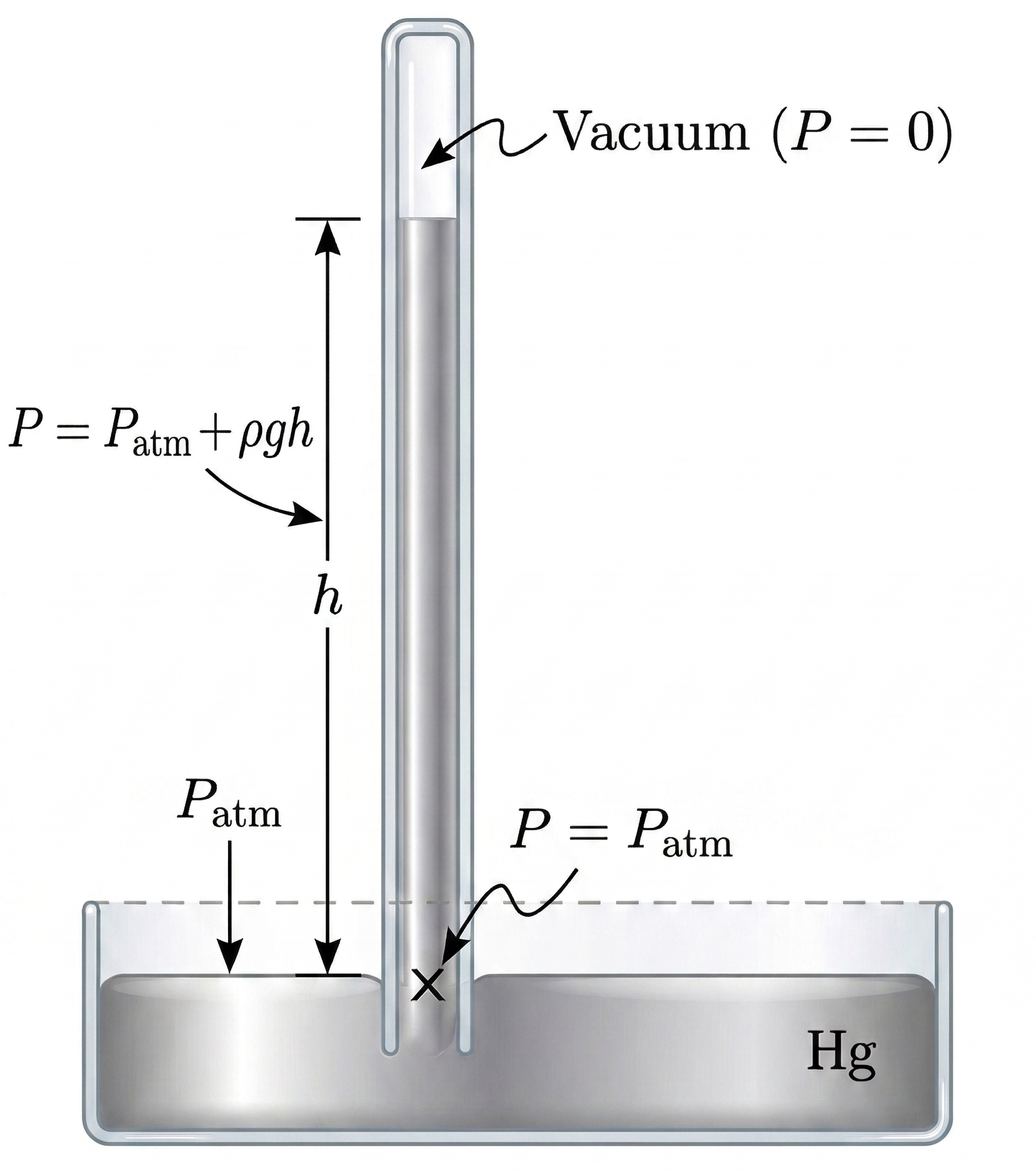
Fig. 14.10 Image Credit: Generated using Gemini.

Weather forecasters closely monitor changes in atmospheric pressure because it signals a change in the weather. The barometer can also be used as an altimeter, since the average atmospheric pressure varies with altitude. Mercury barometers and manometer are common enough so that millimeter heights of mercury (\(\rm mm\ Hg\)) are quoted for atmospheric and blood pressures.

14.2.2.3. Units of pressure

The SI unit for pressure is the pascal (\(\rm Pa\)), where \(1\ {\rm Pa} = 1\ {\rm N/m^2}\). In addition to the pascal, there are many other units for pressure in common use (see Table 14.3). Im meteorology, atmospheric pressure is often describe in the units of millibars (\(\rm mbar\)), where

\[\begin{align*} 1\ {\rm bar} &= 10^5\ {\rm Pa}, \\ 1000\ {\rm mbar} &= 10^5\ {\rm Pa}. \end{align*}\]

The millibar is convenient for meteorologists because the average atmospheric pressure at sea level on Earth is \(1.013 \times 10^5\ {\rm Pa} = 1013\ {\rm mbar} = 1\ {\rm atm}\). Using the equations derived when considering pressure at a depth of fluid, pressure can also be measured as millimeters (or inches) of mercury.

The pressure at the bottom of a \(760{-}{\rm mm}\) column of mercury at \(0^\circ\) in barometer is equal to the atmospheric pressure. Thus, \(760\ {\rm mm\ Hg}\) is also used in place of one atmosphere of pressure.

In vacuum physics labs, scientists often use another unit called \(\rm torr\) (named after Torricelli), where \(1\ {\rm torr} = 1\ {\rm mm\ Hg}\).

Table 14.3 Common Units of Pressure (Referenced to Pascals)

Unit	Equivalent in Pascals
Pascal (Pa)	\(1\ {\rm Pa} = 1\ {\rm N/m^2}\)
pound per square inch (psi)	\(1\ {\rm psi} = 6895\ {\rm Pa}\)
atmosphere (atm)	\(1\ {\rm atm} = 1.013\times10^{5}\ {\rm Pa}\)
bar	\(1\ {\rm bar} = 10^{5}\ {\rm Pa}\)
torr (mm Hg)	\(1\ {\rm torr} = 133.3\ {\rm Pa}\)
inches of mercury (in Hg)	\(1\ {\rm in\ Hg} = 3386\ {\rm Pa}\)
millibar (mbar)	\(1\ {\rm mbar} = 100\ {\rm Pa}\)

14.2.2.4. Example Problem: Fluid Heights in an Open U-Tube

Exercise 14.2

The Problem

A U-tube with both ends open is filled with a liquid of density \(\rho_1\) to a height \(h\) on both sides (Fig. 14.11). A liquid of density \(\rho_2 < \rho_1\) is poured into one side and Liquid 2 settles on top of Liquid 1. The heights on the two sides are different. The height to the top of Liquid 2 from the interface is \(h_2\) and the height to the top of Liquid 1 from the level of the interface is \(h_1\). Derive a formula for the height difference.

Fig. 14.11 Image Credit: Openstax.

Show worked solution

The Model

Because both ends of the tube are open, each free surface is exposed to the same atmospheric pressure \(P_o\). In hydrostatic equilibrium, two points at the same height within the same connected liquid must have the same pressure. We therefore compare the pressure at the interface on the right side to the pressure at a point in Liquid 1 on the left side at that same height. The pressure at each point is the atmospheric pressure plus the weight of the fluid column above it.

The Math

On the left side, the point at the interface level lies beneath a column of Liquid 1 of height \(h_1\), so its pressure is

\[\begin{align*} P_{\rm left} = P_o + \rho_1 g h_1. \end{align*}\]

On the right side, the interface lies beneath a column of Liquid 2 of height \(h_2\), so its pressure is

\[\begin{align*} P_{\rm right} = P_o + \rho_2 g h_2. \end{align*}\]

Because these two points are at the same height in the same connected fluid, their pressures must be equal. Thus,

\[\begin{align*} P_o + \rho_1 g h_1 &= P_o + \rho_2 g h_2. \end{align*}\]

Subtracting \(P_o\) from both sides and dividing by \(g\) gives

\[\begin{align*} \rho_1 h_1 &= \rho_2 h_2. \end{align*}\]

Solving for \(h_1\) gives

\[\begin{align*} h_1 = \frac{\rho_2}{\rho_1} h_2. \end{align*}\]

The height difference between the two sides is therefore

\[\begin{align*} h_2 - h_1 &= h_2 - \frac{\rho_2}{\rho_1} h_2 \\ &= \left(1 - \frac{\rho_2}{\rho_1}\right) h_2. \end{align*}\]

The Conclusion

The height difference between the two fluid levels is

\[\begin{align*} \boxed{h_2 - h_1 = \left(1 - \frac{\rho_2}{\rho_1}\right) h_2.} \end{align*}\]

This result is consistent with the special case \(\rho_2 = \rho_1\), for which the two heights become equal.

The Verification

The algebraic result can be checked by choosing sample densities and a sample value of \(h_2\), then comparing the direct difference \(h_2-h_1\) with the derived formula.

# sample values for the fluid densities (in kg/m^3)
rho_1 = 1000.0   # density of Liquid 1
rho_2 = 800.0    # density of Liquid 2

# sample height of Liquid 2 above the interface (in m)
h_2 = 0.50

# compute the height h_1 from hydrostatic equilibrium
h_1 = (rho_2 / rho_1) * h_2

# compute the height difference directly
delta_h_direct = h_2 - h_1

# compute the height difference from the derived formula
delta_h_formula = (1 - rho_2 / rho_1) * h_2

print(f"The height of Liquid 1 above the interface is {h_1:.3f} m.")
print(f"The direct height difference is {delta_h_direct:.3f} m.")
print(f"The derived formula gives a height difference of {delta_h_formula:.3f} m.")

14.3. Pascal’s Principle and Hydraulics

This audio is AI-generated.

14.3.1. Pascal’s Principle

In 1653, Blaise Pascal published his Treatise on the Equilibrium of Liquids, in which he develops his principles of static fluids. When a fluid is not flowing (i.e., static), we say that the fluid is in static equilibrium. If the fluid is water, we say it is in hydrostatic equilibrium. For a fluid in static equilibrium, the net force on any part of the fluid must be zero because the fluid will would otherwise start to flow.

Pascal’s observations provide the foundation for hydraulics. Pascal observed that a change in pressure applied to an enclosed fluid is transmitted undiminished throughout the fluid and to the walls of the container. Pascal’s principle implies that the total pressure in a fluid is the sum of the pressures from different sources.

Note that this principle does not say that the pressure is the same at all points of a fluid. A good example is the fluid at a depth depends on the depth of the fluid and the pressure of the atmosphere. Rather, Pascal’s principle applies to the change in pressure.

Fig. 14.12 Image Credit: Openstax.

Suppose you place some water in a cylindrical container of height \(h\) and cross-sectional area \(A\) that has a movable piston of mass \(m\) (see Figure 14.12). Adding a weight \(w = Mg\) at the top of the piston increases the pressure at the top by \(w/A = Mg/A\), since the additional weight also acts over the area \(A\) of the lid by

\[ \Delta p_{\rm top} = \frac{Mg}{A}. \]

According to Pascal’s principle, the pressure at all points in the water changes by the same amount, \(Mg/A\). Thus the pressure at the bottom also increases by \(Mg/A\). The pressure at the bottom of the container is equal to the sum of

• the atmospheric pressure,

• the pressure due to the fluid, and

• the pressure supplied by the mass.

The change in pressure at the bottom of the container due to the mass is

\[ \Delta p_{\rm bottom} = \frac{Mg}{A}. \]

Since the pressure changes are the same everywhere in the fluid, we no longer need subscripts to designate the pressure change for the top or bottom, where

\[ \Delta p = \Delta p_{\rm top} = \Delta p_{\rm bottom} = \Delta p_{\rm everywhere}. \]

Physics4Life

This video shows that the pressure only depends on height of fluid on top.

14.3.2. Applications of Pascal’s Principle and Hydraulic Systems

Hydraulic systems are used to operate automotive brakes, hydraulic jacks, and many other mechanical systems (see Figure 14.13). We can derive a relationship between the forces in a simple hydraulic system by applying Pascal’s principle.

Fig. 14.13 Image Credit: Openstax.

The two pistons (in Fig. 14.13) are at the same height, so there is no difference in pressure due to a difference in depth. The pressure due to \(F_1\) action on area \(A_1\) is simply

\[ P_1 = \frac{F_1}{A_1}. \]

According to Pascal’s principle, the pressure is transmitted undiminished throughout the fluid and to all walls of the container. Thus, a pressure \(P_2\) is felt at the other piston that is equal to \(P_1\) (i.e., \(P_1=P_2\)). However, \(P_2 = F_2/A_2\), for this to be so, we find that

(14.10)\[\begin{align} \frac{F_1}{A_1} &= \frac{F_2}{A_2}. \end{align}\]

This equation relates the ratios of force to area in any hydraulic system, provided that the pistons are at the same vertical height and that friction in the system is negligible.

Hydraulic systems can increase or decrease the force applied to them. To mak the force larger, te pressure is applied to a larger area. For example if a \(100\)-\(\rm N\) force is applied to the left cylinder in Figure 14.13 and the right cylinder has an area \(5\times\) greater, then the output force is \(500\ {\rm N}\). Hydraulic systems are analogous to simple levers, but they have the advantage tha pressure can be sent through curved lines to several places at once.

The hydraulic jack is used to lift heavy loads, such as those used by auto mechanics to raise an automobile. It consists of an incompressible fluid filled in a U-tube fitted with a movable piston on each side. One side of the U-tube is narrower than the other. A small force applied over a small area can balance a much larger force on the other side over a larger area (see Figure 14.14).

Fig. 14.14 Image Credit: Openstax.

From Pascal’s principle, we find that the force needed to lift the care is less than the weight of the car:

\[ F_1 = \left(\frac{A_1}{A_2}\right)F_2, \]

where \(F_1\) is the force applied to lift the car, \(A_1\) is the cross-sectional area of the smaller piston, \(A_2\) is the cross-sectional area of the larger piston, and \(F_2\) is the weight of the car.

14.3.3. Example Problem: Calculating Force on Wheel Cylinders

Exercise 14.3

The Problem

Consider the automobile hydraulic system shown in Fig. 14.15. Suppose a force of \(100\ {\rm N}\) is applied to the brake pedal, which acts on the pedal cylinder (acting as a “master” cylinder) through a lever. A force of \(500\ {\rm N}\) is exerted on the pedal cylinder. Pressure created in the pedal cylinder is transmitted to the four wheel cylinders. The pedal cylinder has a diameter of \(0.500\ {\rm cm}\) and each wheel cylinder has a diameter of \(2.50\ {\rm cm}\). Calculate the magnitude of the force \(F_2\) created at each of the wheel cylinders.

Fig. 14.15 Image Credit: OpenStax.

Show worked solution

The Model

We treat the brake fluid as an ideal fluid in static equilibrium, so Pascal’s principle applies. The pressure is transmitted equally throughout the fluid, which means the pressure in the master cylinder equals the pressure in each wheel cylinder. If \(F_1\) is the force applied to the pedal cylinder, and \(A_1\) and \(A_2\) are the cross-sectional areas of the pedal and wheel cylinders, respectively, then \(F_1/A_1 = F_2/A_2\). Because the given \(500\ {\rm N}\) is already the force exerted on the pedal cylinder, the lever analysis is not needed here.

---

The Math

We begin with Pascal’s principle, which states that the pressure is the same in both cylinders. This gives the relationship \(F_1/A_1 = F_2/A_2\), where \(F_1\) is the force applied to the pedal cylinder and \(F_2\) is the force exerted by each wheel cylinder. Solving this equation for the output force gives \(F_2 = (A_2/A_1)F_1\).

Because both cylinders have circular cross sections, their areas can be written in terms of their radii as \(A = \pi r^2\). Substituting this into the area ratio shows that the factor \(\pi\) cancels, leaving \(A_2/A_1 = r_2^2/r_1^2\). This allows us to express the force entirely in terms of the cylinder radii.

The given diameters of the pedal and wheel cylinders are \(0.500\ {\rm cm}\) and \(2.50\ {\rm cm}\), respectively, so the corresponding radii are \(r_1 = 0.250\ {\rm cm}\) and \(r_2 = 1.25\ {\rm cm}\). Substituting these values into the force relation gives

\[\begin{align*} F_2 &= \left(\frac{r_2^2}{r_1^2}\right) F_1 \\ &= \left(\frac{(1.25\ {\rm cm})^2}{(0.250\ {\rm cm})^2}\right)(500\ {\rm N}) \\ &= 25(500\ {\rm N}) \\ &= 1.25\times10^{4}\ {\rm N}. \end{align*}\]

---

The Conclusion

Each wheel cylinder exerts a force of \(1.25\times10^{4}\ {\rm N}\). This result is significantly larger than the \(500\ {\rm N}\) force applied to the pedal cylinder, which reflects the large ratio of the cylinder areas in the hydraulic system. Because pressure is transmitted equally throughout the fluid, increasing the cross-sectional area of the output cylinder increases the force it exerts.

This amplification of force explains how a driver can apply a relatively small force at the pedal and still generate a much larger braking force at the wheels. However, this increase in force comes at the expense of distance—the wheel cylinders move a smaller distance than the pedal cylinder, so the total work done remains consistent with energy conservation.

---

The Verification

The code below computes the area ratio from the cylinder radii and then uses Pascal’s principle to calculate the force produced by each wheel cylinder.

import numpy as np

# given values
F1 = 500.0       # force applied to the pedal cylinder (N)
r1 = 0.250       # radius of the pedal cylinder (cm)
r2 = 1.25        # radius of each wheel cylinder (cm)

# compute the area ratio A2/A1 for circular cylinders
area_ratio = r2**2 / r1**2

# compute the output force at each wheel cylinder
F2 = area_ratio * F1

print(f"The area ratio of the wheel cylinder to the pedal cylinder is {area_ratio:.1f}.")
print(f"The force exerted by each wheel cylinder is {F2:.3e} N.")

14.4. Archimedes’ Principle and Buoyancy

This audio is AI-generated.

When placed in a fluid, some objects float due to a buoyant force (see Figure 14.16).

• Where does this buoyant force come from?

• Why is it that some things float and others do not?

• Do objects that sink get any support at all from the fluid?

• Is your body buoyed by the atmosphere, or are helium balloons affected?

Fig. 14.16 Image Credit: Openstax.

Pressure increases with depth in a fluid!

This means that the upward force on the bottom of an object (in a fluid) is greater than the downward force on top of the object. There is an upward, or buoyant, force on any object in any fluid (see Figure 14.17).

Fig. 14.17 Image Credit: Openstax.

• If the buoyant force is greater than the object’s weight, the net force on the object is upward. If we release such an object, it will rise in the fluid.

• If the buoyant force is less than the object’s weight, the object sinks when released.

• If the buoyant force equals the object’s weight, the object can remain suspended at its present depth, either immersed in the fluid or partly above the surface.

The buoyant force is always present, whether the object floats, sinks, or is suspended in a fluid.

Buoyant Force

The buoyant force is the upward force on any object in any fluid.

14.4.1. Archimedes’ Principle

Just how large is the buoyant force?

Consider what happens when a submerged object is removed from a fluid (see Figure 14.18). If the object were not in the fluid, the space the object occupied would be filled by fluid having a weight \(w_{\rm fl}\). This weight is supported by the surrounding fluid, so the buoyant force must equal \(w_{\rm fl}\), or the weight of the fluid displaced by the object.

Fig. 14.18 Image Credit: Openstax.

Archimedes’ Principle

The buoyant force on an object equals the weight of the fluid it displaces. In equation form, Archimedes’ principle is

\[ F_{\rm B} = w_{\rm fl}, \]

where \(F_{\rm B}\) is the buoyant force and \(w_{\rm fl}\) is the weight of the fluid displaced by the object.

This principle is named after the Greek mathematician and inventor Archimedes of Syracuse, who state this principle long before concepts of force were well established.

Archimedes’ principle refers to the force of buoyancy that results when a body is submerged in a fluid, whether partially or wholly. The force that provides the pressure of a fluid acts on a body perpendicular to the surface. The force due to the pressure at the bottom is pointed up, while at the tope, the force due to the pressure is pointed down. The forces due to pressures at the sides are pointing into the body.

Since the bottom of the body is at a greater depth than the top, the pressure at the lower part of the body is higher than the pressure at the upper part (as shown in Fig. 14.17). Therefore a net upward force acts on the body. This upward force is the force of buoyancy.

TEDEd

This video tells the tale of Archimedes and his famous phrase Eureka!

14.4.2. Density and Archimedes’ Principle

If you drop a lump of clay in water, it will sink. But if you mold the same lump of clay into the shape of a boat, then it will float. The clay boat displaces more water than the lump and experiences a greater buoyant force, even though its mass is the same.

The average density of an object is what ultimately determines whether it floats. If an object’s average density is less than that of the surrounding fluid, it will float. The fluid has a higher density, which means contains more mass for a given volume and hence more weight. The buoyant force is greater than the weight of the object. An object denser than the fluid will sink.

In Figure 14.19, the unloaded ship has a lower density and less of it is submerged compared with the loaded ship. We can derive a quantitative expression for the fraction submerged by considering density.

Fig. 14.19 Image Credit: Openstax.

The fraction submerged is the ratio of the volume submerged to the volume of the object, or

\[ \text{fraction submerged} = \frac{V_{\rm sub}}{V_{\rm obj}} = \frac{V_{\rm fl}}{V_{\rm obj}}. \]

The volume submerged \(V_{\rm sub}\) equals the volume of the fluid displaced \(V_{\rm fl}\). We can obtain the relationship between the densities by substituting \(\rho = m/V\), or \(V= m/\rho\). This gives

\[ \frac{V_{\rm fl}}{V_{\rm obj}} = \left(\frac{m_{\rm fl}}{\rho_{\rm fl}}\right) \left(\frac{\rho_{\rm obj}}{m_{\rm obj}}\right) = \left(\frac{m_{\rm fl}}{m_{\rm obj}}\right) \left(\frac{\rho_{\rm obj}}{\rho_{\rm fl}}\right),\]

where \(\rho_{\rm obj}\) is the average density of the object and \(\rho_{\rm fl}\) is the density of the fluid. Since the object floats, its mass and that of the fluid displaced are equal (i.e., \(m_{\rm obj} = m_{\rm fl}\)), leaving

\[ \frac{V_{\rm fl}}{V_{\rm obj}} = \frac{\rho_{\rm obj}}{\rho_{\rm fl}}.\]

We can determine the density of an unknown fluid using an object of a known density and measuring the fraction of it that is submerged.

Numerous lower-density objects or substances float in higher density fluids, such as:

• oil on water,

• a hot-air ballon in the atmosphere,

• a bit of cork in wine,

• an iceberg in salt water, and

• hot wax in a “lava lamp.

A less obvious example is that mountain ranges float on the higher density crust and mantle beneath them.

14.4.3. Measuring Density

A common technique to measure density is to use a scale balance (see Figure 14.20), where you weigh the object (e.g., a coin) in air and then weigh it again submerged in a liquid of known density (e.g., water). The density of the object can be calculated and your (fool’s) gold can be authenticated.

Fig. 14.20 Image Credit: Openstax.

This calculation is based on Archimedes’ principle, where the buoyant force on an object is equal to the weight of the fluid it displaces. This means that the object appears to weigh less when submerged. The weight measured while submerged is called the object’s apparent weight.

The object suffers an apparent weight loss equal to the weight of the fluid displaced. On balances that measure mass, the object suffers an apparent mass loss equal to the mass of fluid displaced.

14.4.4. Example Problem: Calculating Average Density

Exercise 14.4

The Problem

Suppose a \(60.0\ {\rm kg}\) woman floats in fresh water with \(97.0\%\) of her volume submerged when her lungs are full of air. What is her average density?

Show worked solution

The Model

When an object floats at rest, the buoyant force balances its weight. The buoyant force equals the weight of the displaced fluid, so \(\rho_{\rm fl} g V_{\rm sub} = \rho_{\rm obj} g V\). The fraction of the object’s volume that is submerged is therefore determined by the ratio of densities.

---

The Math

For an object in equilibrium, the buoyant force equals the weight, so \(\rho_{\rm fl} g V_{\rm sub} = \rho_{\rm obj} g V\). Dividing both sides by \(\rho_{\rm fl} g V\) gives

\[\begin{align*} \frac{V_{\rm sub}}{V} = \frac{\rho_{\rm obj}}{\rho_{\rm fl}}. \end{align*}\]

The problem states that \(97.0\%\) of the volume is submerged, so \(V_{\rm sub}/V = 0.970\). Solving for the density of the woman gives

\[\begin{align*} \rho_{\rm obj} = \left(\frac{V_{\rm sub}}{V}\right)\rho_{\rm fl}. \end{align*}\]

Substituting the known values with \(\rho_{\rm fl} = 1000\ {\rm kg/m^3}\) gives

\[\begin{align*} \rho_{\rm obj} = (0.970)(1000\ {\rm kg/m^3}) = 970\ {\rm kg/m^3}. \end{align*}\]

---

The Conclusion

The woman’s average density is \(970\ {\rm kg/m^3}\). This value is slightly less than the density of water, which is why she floats with most—but not all—of her volume submerged. The fact that \(97.0\%\) of her volume is below the surface directly reflects how close her density is to that of water.

---

The Verification

The calculation can be checked by comparing the weight of the woman to the buoyant force computed from the displaced volume fraction.

# given values
rho_fl = 1000      # density of water (kg/m^3)
fraction_sub = 0.970  # fraction of volume submerged

# compute density of the woman
rho_obj = fraction_sub * rho_fl

print(f"The average density of the woman is {rho_obj:.0f} kg/m^3.")

14.5. Fluid Dynamics

This audio is AI-generated.

In contrast to static fluids, there is the study of fluids in motion or fluid dynamics. Even the most basic forms of fluid motion can be quite complex. For this reason, we limit our investigation to ideal fluids in many of the examples. In ideal fluid is a fluid with negligible viscosity, where viscosity is a measure of the internal friction in a fluid.

14.5.1. Characteristics of Flow

Velocity vectors are often used to illustrate fluid motion in applications like meteorology. Wind can be modeled as a fluid motion of air in the atmosphere and represented by vectors indicating the speed and direction of the wind at any given point on a map. Figure 14.21 shows velocity vectors describing the winds during Hurricane Arthur in 2014.

Fig. 14.21 Image Credit: Openstax.

Another method for representing fluid motion is a streamline. A streamline represents the path of a small volume of fluid as it flows. The velocity is always tangential to the streamline. Figure 14.22 illustrates two examples of fluids moving through a pipe.

Fig. 14.22 Image Credit: Openstax.

There are two extremes of fluid flow:

• laminar flow (sometimes called steady flow) is represented by smooth, parallel streamlines. The velocity of the fluid is greatest in the center and decreases near the walls of the pipe. The gradient in velocity is due to the viscosity of the fluid and friction between the pipe walls and the fluid.

• turbulent flow has streamlines that are irregular and change over time. In turbulent flow the paths of the fluid flow are irregular as different parts of the fluid mix together or form small circular regions that resemble whirlpools.

14.5.2. Flow Rate and its Relation to Velocity

The volume of fluid passing by a given location through an area during a period of time is called the flow rate \(Q\), or volume flow rate. This is written as

(14.11)\[\begin{align} Q = \frac{dV}{dt}, \end{align}\]

where \(V\) is the volume and \(t\) is the elapsed time.

Fig. 14.23 Image Credit: Openstax.

In Figure 14.23, the volume of the cylinder is \(Ax\) and thus, the flow rate is

\[ Q = \frac{dV}{dt} = \frac{d}{dt}(Ax) = A \frac{dx}{dt} = Av. \]

The SI unit for flow rate is \(\rm m^3/s\), but several other units are in common use, such as liters per minute (\(\rm L/min\)).

Flow rate and velocity are related, but measure different physical quantities. To make the distinction clear, consider the flow rate of a river. The greater the velocity of the water, the greater the flow rate of the river. Flow rate depends on the size and shape of the river. A rapid mountain stream carries far less water than the Amazon River.

Figure 14.23 illustrates the volume flow rate, which is given by \(Q = \frac{dV}{dt} = Av\) and depends on the cross-sectional area \(A\) of the pipe, as well as the average speed \(v\). The relationship tells us that the larger the conduit, the greater its cross-sectional area. In Fig. Figure 14.23, the shaded cylinder has a volume \(V = Ad\), which flows past the point \(P\) in a time \(t\). Dividing both sides by \(t\) gives

\[ \frac{V}{t} = \frac{Ad}{t}.\]

Since the average speed is given by \(v=d/t\) and the flow rate is the changing volume over time (\(Q = V/t\)), this means that \(Q = Av\).

Fig. 14.24 Image Credit: Openstax.

Figure 14.24 shows an incompressible fluid flowing along a pipe of decreasing radius. Because the fluid is incompressible, the same amount of fluid must flow past any point in the tube in a given time to ensure continuity of flow. The flow is continuous because there are no sources (or sinks) to add (or remove) mass. The mass flowing into the pipe must equal the mass flowing out of the pipe.

In this case, the cross-sectional area of the pipe decreases and the velocity must necessarily increase. This logic can be extended to say that the flow rate must be the same at all points along the pipe. In particular for two arbitrary points \(1\) and \(2\), we have

(14.12)\[\begin{align} Q_1 &= Q_2, \\ A_1v_1 &= A_2v_2. \end{align}\]

This is called the equation of continuity and is valid for any incompressible fluid (with constant density). Consider how water flows from a narrow spray nozzle: The water emerges with a large speed when the area of the nozzle is restricted. Conversely, when a river empties into one end of a reservoir, the water slows considerably and can pickup speed again when it leaves the other end of the reservoir. Speed increases when the cross-sectional area decreases, and vice-versa.

Liquids are essentially incompressible, which makes the equation of continuity valid for all liquids. however gases are compressible, so the the equation must be applied with caution to gases as they are subjected to compression or expansion.

14.5.3. Mass Conservation

The flow rate of a fluid can also be described by the mass flow rate. This is the rate at which a mass of the fluid moves past a fixed point. Consider the mass within the shaded volume of Figure 14.23. The mass can be determined from the density and volume:

\[ m = \rho V = \rho Ax. \]

The mass flow rate is then defined by

\[ \frac{dm}{dt} = \frac{d}{dt}\left(\rho Ax\right) = \rho A\frac{dx}{dt} = \rho Av, \]

where \(\rho\) is the density, \(A\) is the cross-sectional area, and \(v\) is the speed (i.e., magnitude of velocity). The mass flow rate can be used to solve problems using equation of continuity. Consider the pipe (in Fig. 14.24), where the inlet has a cross-sectional area \(A_1\) and the outlet constricts with an cross sectional area \(A_2\). From continuity, the total mass entering the pipe must be equal to the mass of fluid exiting the pipe.

We can find a relationship between the velocity and the cross-sectional area by setting the inlet mass flow rate equal to the outlet mass flow rate:

(14.13)\[\begin{align} \rho_1 A_1 v_1 &= \rho_2 A_2 v_2. \end{align}\]

This is also known as the general form of the continuity equation. If the density of the fluid remains constant through the constriction (i.e., the fluid is incompressible), then the density cancels from the continuity equation,

\[ A_1 v_1 = A_2 v_2. \]

The equation reduces to show the volume flow rate into the pipe equals the volume flow rate out of the pipe.

14.5.4. Example Problem: Calculating Fluid Speed through a Nozzle

Exercise 14.5

The Problem

A nozzle with a diameter of \(0.500\ {\rm cm}\) is attached to a garden hose with a radius of \(0.900\ {\rm cm}\). The flow rate through hose and nozzle is \(0.500\ {\rm L/s}\). Calculate the speed of the water (a) in the hose and (b) in the nozzle.

Show worked solution

The Model

We model the water as an incompressible fluid flowing steadily through the hose and nozzle. Because the fluid is incompressible, the volume flow rate is conserved between different cross sections. The hose and nozzle are both treated as circular pipes, so their cross-sectional areas depend only on their radii. The given flow rate determines the fluid speed in each section through the geometry of the pipe.

---

The Math

(a) To determine the speed of the water in the hose, we begin with the definition of volume flow rate, which relates the flow rate to the cross-sectional area and the fluid speed. Solving this relationship for the speed allows us to express the velocity in terms of the known flow rate and the area of the hose.

\[\begin{align*} v_1 &= \frac{Q}{A_1}. \end{align*}\]

The hose has a radius of \(r_1 = 0.900\ {\rm cm} = 9.00\times10^{-3}\ {\rm m}\), so its cross-sectional area is \(A_1 = \pi r_1^2\). The flow rate is \(Q = 0.500\ {\rm L/s} = 5.00\times10^{-4}\ {\rm m^3/s}\). Substituting these values gives

\[\begin{align*} v_1 &= \frac{Q}{\pi r_1^2} \\ &= \frac{5.00\times10^{-4}\ {\rm m^3/s}}{\pi (9.00\times10^{-3}\ {\rm m})^2} \\ &= 1.96\ {\rm m/s}. \end{align*}\]

(b) To determine the speed in the nozzle, we use the continuity condition, which states that the flow rate is the same through both sections of the pipe. This implies that the product of cross-sectional area and speed is constant, so solving for the nozzle speed gives

\[\begin{align*} v_2 &= \frac{A_1}{A_2} v_1. \end{align*}\]

Because both cross sections are circular, the ratio of areas can be expressed in terms of the radii, which allows us to write

\[\begin{align*} \frac{A_1}{A_2} = \frac{r_1^2}{r_2^2}. \end{align*}\]

The nozzle diameter is \(0.500\ {\rm cm}\), so its radius is \(r_2 = 0.250\ {\rm cm}\). Substituting the known values gives

\[\begin{align*} v_2 &= \left(\frac{r_1^2}{r_2^2}\right) v_1 \\ &= \left(\frac{(0.900\ {\rm cm})^2}{(0.250\ {\rm cm})^2}\right)(1.96\ {\rm m/s}) \\ &= 25.4\ {\rm m/s}. \end{align*}\]

---

The Conclusion

The speed of the water in the hose is \(1.96\ {\rm m/s}\), and the speed in the nozzle is \(25.4\ {\rm m/s}\). The much higher speed in the nozzle is a direct consequence of the smaller cross-sectional area, since the same volume flow rate must pass through both sections. This illustrates how constricting a fluid flow increases its speed.

---

The Verification

The calculation computes the fluid speed in the hose using the flow rate and cross-sectional area, then applies continuity to determine the speed in the nozzle. This mirrors the analytical method used above.

import numpy as np

# given values
Q = 5.00e-4      # flow rate (m^3/s)
r1 = 9.00e-3     # hose radius (m)
r2 = 2.50e-3     # nozzle radius (m)

# compute cross-sectional areas
A1 = np.pi * r1**2
A2 = np.pi * r2**2

# compute speeds
v1 = Q / A1
v2 = (A1 / A2) * v1

print(f"The speed of the water in the hose is {v1:.2f} m/s.")
print(f"The speed of the water in the nozzle is {v2:.1f} m/s.")

14.6. Bernoulli’s Equation

This audio is AI-generated.

When a fluid flows into a narrower channel, its speed increases which means that its kinetic energy increases as well. The increased kinetic energy come from the net work don on the fluid to push it into the channel. If the fluid changes vertical position, work is also done on the fluid by the gravitational force.

A pressure difference occurs when the channel narrows, where this difference results in a net force on the fluid because the \(P \times A = F\), and this net force does work. Recall the work-energy theorem,

\[ W_{\rm net} = \Delta K = K - K_o = \frac{1}{2}mv^2 - \frac{1}{2}mv_o^2. \]

The net work done increases the fluid’s kinetic energy. As a result, the pressure drops in a rapidly moving fluid whether or not the fluid is confined to a tube.

For example, shower curtains have a disagreeable habit of bulging into the shower stall when the shower is on. The high-velocity stream of water and air creates a region of lower pressure inside the shower, whereas the pressure on the other side remains the same (at the standard atmospheric pressure). This pressure difference results in a net force, pushing the curtain inward.

Similarly, when a car passes a semi on the highway, the two vehicles pull toward each other. The reason is the same: The high velocity of the air between the car and the truck creates a region of lower pressure between the vehicles, and they are pushed together by greater pressure on the outside (see Figure 14.25). THis effect was observed as back as the mid-1800s, when it was found that trains passing in opposite directions tipped precariously toward one another.

Fig. 14.25 Image Credit: Openstax.

14.6.1. Energy Conservation and Bernoulli’s Equation

The application of the principle of conservation of energy to frictionless laminar flow leads to a very useful relation between pressure and a fluid’s flow speed. This relation is called Bernoulli’s equation, named after Daniel Bernoulli who published his studies in his book Hydrodynamica.

Consider an incompressible fluid flowing through a pipe that has a varying diameter and height (see Figure 14.26). We identify two locations along the pipe using the subscripts \(1\) and \(2\) on the respective physical parameters: cross-sectional area, velocity, height, and pressure. We assume that the density at the two points is the same, where the shaded volumes must be equal since the fluid is incompressible.

Fig. 14.26 Image Credit: Openstax.

We also assume that there are no viscous forces in the fluid, so the energy of any part of the fluid will be conserved. To derive Bernoulli’s equation, we first calculate the work that was done on the fluid:

\[\begin{align*} dW &= F_1 dx_1 - F_2 dx_2, \\ &= P_1 A_1 dx_1 - P_2 A_2 dx_2, \\ &= P_1 dV - P_2 dV = (P_1 - P_2)dV. \end{align*}\]

The work done was due to the conservative force of gravity and the change in the kinetic energy of the fluid. The change in the kinetic energy of the fluid is equal to

\[ \Delta K = \frac{1}{2}m_2v_2^2 - \frac{1}{2}m_1 v_1^2 = \frac{\rho}{2}dV\left(v_2^2 -v_1^2\right), \]

where we have used the relation \(m = \rho dV\). The change in potential energy is

\[ \Delta U = mgh_2 - mgh_1 = \rho dV g(h_2-h_1). \]

The energy equation then becomes

\[\begin{align*} dW &= \Delta K + \Delta U, \\ (P_1 - P_2)dV &= \frac{\rho}{2}dV\left(v_2^2 -v_1^2\right) + \rho dV g(h_2-h_1), \\ P_1 - P_2 &= \frac{1}{2}\rho\left(v_2^2 -v_1^2\right) + \rho g(h_2-h_1). \end{align*}\]

Rearranging the equation gives Bernoulli’s equation:

\[ P_1 + \frac{1}{2}\rho v_1^2 + \rho gh_1 = P_2 + \frac{1}{2}\rho v_2^2 + \rho gh_2. \]

This relation states that the mechanical energy of any part of the fluid changes as a result of the work done by the fluid external to that part, du to varying the pressure along the way. Since the two points were chosen arbitrarily, we can write Bernoulli’s equation more generally as a conservation principle along the flow.

Bernoulli’s Equation

For an ideal fluid moving steadily, the pressure and energy density is conserved along a flow line. The conservation relation is given by

(14.14)\[\begin{align} P + \frac{1}{2}\rho v^2 + \rho gh = \text{constant}, \end{align}\]

where \(P\) is the pressure, \(\rho\) is the mass density, \(v\) is the speed of the fluid, and \(h\) is the height.

In a dynamic situation, the pressures at the same height in different parts of the fluid may be different if they have different speeds of flow.

14.6.2. Analyzing Bernoulli’s Equation

If we follow a small volume of fluid along its path, the sum of pressure and energy density remains the same even though various individual quantities may change. Bernoulli’s equation is just a convenient statement of the conservation of energy for an incompressible fluid in the absence of friction.

14.6.2.1. Bernoulli’s equation for static fluids

Consider the simple solution where the fluid is static (i.e., \(v_1 = v_2 = 0\)). Bernoulli’s equation in that case is

\[ P_1 + \rho gh_1 = P_2 + \rho gh_2. \]

We can simplify the equation by measuring the relative height \(h\) as the difference between \(h_2\) and \(h_1\), or \(h = h_2 - h_1\). In this case, we get

\[ P_2 = P_1 + \rho gh. \]

This equation tells us tha the pressure increases with depth for static fluids. As we go from point \(1\) to point \(2\) in the fluid, the depth increases by \(h\) and the difference in pressure is equal to \(\rho gh\). Thus, Bernoulli’s equation confirms the fact that pressure change due to the weight of a fluid is \(\rho gh\).

14.6.2.2. Bernoulli’s principle

Suppose a fluid is moving but its depth is constant (i.e, \(h_1 = h_2\)). Under this condition, Bernoulli’s equation becomes

\[ P_1 + \frac{1}{2}\rho v_1^2 = P_2 + \frac{1}{2}\rho v_2^2. \]

Situations in which fluid flows at a constant depth are so common that this equation is often called Bernoulli’s principle, which is simply Bernoulli’s equation for a constant depth. Bernoulli’s principle reinforces that pressure drops as the speed increases in a moving fluid: If \(v_2>v_1\) in the equation, then \(P_2\) must be less than \(P_1\) for the equality to hold. It is more easily seen by

\[ P_1 - P_2 = \frac{1}{2}\rho (v_2^2 - v_1^2), \]

because \(v^2>0\) and \(P_1 > P_2\) must be true for the left-side to be positive.

14.6.2.3. Example Problem: Calculating Pressure

Exercise 14.6

The Problem

In Example 14.5, we found that the speed of water in a hose increased from \(1.96\ {\rm m/s}\) to \(25.5\ {\rm m/s}\) going from the hose to the nozzle. Calculate the pressure in the hose, given that the absolute pressure in the nozzle is \(1.01\times10^{5}\ {\rm N/m^2}\) (atmospheric, as it must be) and assuming level, frictionless flow.

Show worked solution

The Model

We model the fluid as incompressible and flowing steadily, so Bernoulli’s principle applies along a streamline. Because the flow is level, there is no change in gravitational potential energy. The pressure and kinetic energy of the fluid therefore trade off as the speed changes between the hose and the nozzle. The pressure at the nozzle is atmospheric because the fluid is exposed to the air.

---

The Math

We begin with Bernoulli’s principle, which relates the pressure and speed of the fluid at two points along the same streamline. Because the flow is level, the gravitational terms cancel, leaving a relationship between pressure and kinetic energy.

\[\begin{align*} P_1 + \frac{1}{2}\rho v_1^2 = P_2 + \frac{1}{2}\rho v_2^2. \end{align*}\]

To determine the pressure in the hose, we solve this equation for \(P_1\) by isolating it on one side. Subtracting the kinetic energy term at point 1 and adding the kinetic energy term at point 2 gives

\[\begin{align*} P_1 = P_2 + \frac{1}{2}\rho v_2^2 - \frac{1}{2}\rho v_1^2. \end{align*}\]

Factoring out the common coefficient simplifies the expression to

\[\begin{align*} P_1 = P_2 + \frac{1}{2}\rho\left(v_2^2 - v_1^2\right). \end{align*}\]

The known values are \(P_2 = 1.01\times10^{5}\ {\rm N/m^2}\), \(\rho = 1000\ {\rm kg/m^3}\), \(v_1 = 1.96\ {\rm m/s}\), and \(v_2 = 25.5\ {\rm m/s}\). Substituting these values gives

\[\begin{align*} P_1 &= 1.01\times10^{5}\ {\rm N/m^2} + \frac{1}{2}(1000\ {\rm kg/m^3})\left[(25.5\ {\rm m/s})^2 - (1.96\ {\rm m/s})^2\right] \\ &= 1.01\times10^{5}\ {\rm N/m^2} + 500\left(650.25 - 3.84\right) \\ &= 1.01\times10^{5}\ {\rm N/m^2} + 3.23\times10^{5}\ {\rm N/m^2} \\ &= 4.24\times10^{5}\ {\rm N/m^2}. \end{align*}\]

---

The Conclusion

The pressure in the hose is P_1 = 4.24\times10^{5}\ {\rm N/m^2}. This pressure is greater than atmospheric pressure because the fluid is moving more slowly in the hose than in the nozzle. As the fluid accelerates into the narrower nozzle, kinetic energy increases, which requires a decrease in pressure according to Bernoulli’s principle. This result is consistent with the expectation that higher-speed flow corresponds to lower pressure.

---

The Verification

The calculation evaluates Bernoulli’s equation using the given speeds and fluid density to compute the pressure difference between the hose and nozzle. This directly mirrors the analytical steps shown above.

import numpy as np

# given values
P2 = 1.01e5     # nozzle pressure (Pa)
rho = 1000      # density of water (kg/m^3)
v1 = 1.96       # hose speed (m/s)
v2 = 25.5       # nozzle speed (m/s)

# compute pressure in the hose using Bernoulli's equation
P1 = P2 + 0.5 * rho * (v2**2 - v1**2)

print(f"The pressure in the hose is {P1:.3e} N/m^2.")

14.6.3. Applications of Bernoulli’s Principle

14.6.3.1. Entrainment

People have long put the Bernoulli principle to work by using the reduced pressure in high-velocity fluids to move things around. With a higher pressure on the outside, the high-velocity fluid forces other fluids into the stream. This process is called entrainment. Entrainment devices (see Figure 14.27) have been in use as pumps to raise water to small heights, as needed for draining swamps, field, or other low-lying areas.

Fig. 14.27 Image Credit: Openstax.

14.6.3.2. Velocity measurement

The fluid velocity can be measured with devices making use of Bernoulli’s principle (see Figure 14.28). The manometer (in Fig. 14.28a) is connected to two tube that are small enough to not appreciably disturb the flow. The tube facing the oncoming fluid creates a dead spot having zero velocity (\(v_1=0\)) in front of it, while fluid passing the other tube has a velocity \(v_2\).

Fig. 14.28 Image Credit: Openstax.

This means that Bernoulli’s principle can be simplified by

\[\begin{align*} P_1 + \frac{1}{2}\rho v_1^2 &= P_2 + \frac{1}{2}\rho v_2^2, \\ P_1 &= P_2 + \frac{1}{2}\rho v_2^2, \\ P_2 &= P_1 - \frac{1}{2}\rho v_2^2. \end{align*}\]

Thus, the pressure \(P_2\) over the second opening is reduced by \(\frac{1}{2}\rho v_2^2\), so the fluid in the manometer rises by \(h\) on the side connected to the second opening, where

\[ h \propto \frac{1}{2}\rho v_2^2. \]

Solving for \(v_2\), we see that

\[ v_2 \propto \sqrt{h}. \]

Fig. 14.28b shows a version of this device that is in common use for measuring various fluid velocities, where such devices are frequently used as air-speed indicators in aircraft.

14.6.3.3. Example Problem: A Fire Hose Nozzle

Exercise 14.7

The Problem

Fire hoses used in major structural fires have an inside diameter of \(6.40\ {\rm cm}\) (Fig. 14.29). Suppose such a hose carries a flow of \(40.0\ {\rm L/s}\), starting at a gauge pressure of \(1.62\times10^{6}\ {\rm N/m^2}\). The hose rises up \(10.0\ {\rm m}\) along a ladder to a nozzle having an inside diameter of \(3.00\ {\rm cm}\). What is the pressure in the nozzle?

Fig. 14.29 Image Credit: Openstax.

Show worked solution

The Model

We model the water as an incompressible fluid in steady, frictionless flow, so Bernoulli’s principle applies along a streamline. The hose and nozzle are treated as circular pipes, so the fluid speeds can be found from the volume flow rate and the cross-sectional areas. Because the nozzle is higher than the hose, the pressure at the nozzle is reduced both by the gain in gravitational potential energy and by the increase in kinetic energy as the flow enters the narrower opening. The given initial pressure is a gauge pressure, so the final result will also be a gauge pressure.

---

The Math

To determine the nozzle pressure, we first need the fluid speeds in the hose and in the nozzle. For steady incompressible flow, the volume flow rate is the same at every cross section, so the speed is found from the flow-rate relation \(Q = Av\). Solving for the speed gives \(v = Q/A\).

The hose has diameter \(6.40\ {\rm cm}\), so its radius is \(r_1 = 3.20\ {\rm cm} = 3.20\times10^{-2}\ {\rm m}\). The nozzle has diameter \(3.00\ {\rm cm}\), so its radius is \(r_2 = 1.50\ {\rm cm} = 1.50\times10^{-2}\ {\rm m}\). The flow rate is \(Q = 40.0\ {\rm L/s} = 4.00\times10^{-2}\ {\rm m^3/s}\). Using \(A = \pi r^2\), the speed in the hose is

\[\begin{align*} v_1 &= \frac{Q}{A_1} \\ &= \frac{Q}{\pi r_1^2} \\ &= \frac{4.00\times10^{-2}\ {\rm m^3/s}}{\pi(3.20\times10^{-2}\ {\rm m})^2} \\ &= 12.4\ {\rm m/s}. \end{align*}\]

Using the same method, the speed in the nozzle is

\[\begin{align*} v_2 &= \frac{Q}{A_2} \\ &= \frac{Q}{\pi r_2^2} \\ &= \frac{4.00\times10^{-2}\ {\rm m^3/s}}{\pi(1.50\times10^{-2}\ {\rm m})^2} \\ &= 56.6\ {\rm m/s}. \end{align*}\]

Now that the speeds are known, we apply Bernoulli’s principle between the hose at ground level and the nozzle at the top of the ladder. For steady, incompressible, frictionless flow along a streamline, Bernoulli’s equation is

\[\begin{align*} P_1 + \frac{1}{2}\rho v_1^2 + \rho g h_1 = P_2 + \frac{1}{2}\rho v_2^2 + \rho g h_2. \end{align*}\]

To determine the pressure in the nozzle, we solve this equation for \(P_2\). Taking the hose level as the reference height gives \(h_1 = 0\) and \(h_2 = 10.0\ {\rm m}\). Moving the kinetic-energy and gravitational terms to the other side gives

\[\begin{align*} P_2 &= P_1 + \frac{1}{2}\rho\left(v_1^2 - v_2^2\right) - \rho g h_2,\\ &= 1.62\times10^{6}\ {\rm N/m^2} + \frac{1}{2}(1000\ {\rm kg/m^3})\left[(12.4\ {\rm m/s})^2 - (56.6\ {\rm m/s})^2\right] - (1000\ {\rm kg/m^3})(9.81\ {\rm m/s^2})(10.0\ {\rm m}) \\ &= -2.96\times10^{3}\ {\rm N/m^2}. \end{align*}\]

---

The Conclusion

The pressure in the nozzle is \(-2960\ {\rm N/m^2}\), which is equivalent to \(-2.96\ {\rm kPa}\) gauge pressure. This result is very close to zero compared with atmospheric pressure, which is consistent with the fact that the water is about to emerge into the open air. The large drop in pressure occurs because the water both rises to a higher elevation and speeds up substantially as it enters the narrower nozzle.

---

The Verification

The code below first computes the fluid speeds from the flow rate and the circular cross-sectional areas, then substitutes those values into Bernoulli’s equation to compute the nozzle pressure. This mirrors the analytical solution directly.

import numpy as np

# given values
Q = 4.00e-2      # flow rate (m^3/s)
P1 = 1.62e6      # initial gauge pressure (Pa)
rho = 1000       # density of water (kg/m^3)
g = 9.81         # gravitational acceleration (m/s^2)
r1 = 3.20e-2     # hose radius (m)
r2 = 1.50e-2     # nozzle radius (m)
h1 = 0.0         # hose height (m)
h2 = 10.0        # nozzle height (m)

# compute cross-sectional areas
A1 = np.pi * r1**2
A2 = np.pi * r2**2

# compute fluid speeds
v1 = Q / A1
v2 = Q / A2

# compute nozzle pressure from Bernoulli's equation
P2 = P1 + 0.5 * rho * (v1**2 - v2**2) - rho * g * (h2 - h1)

print(f"The speed of the water in the hose is {v1:.1f} m/s.")
print(f"The speed of the water in the nozzle is {v2:.1f} m/s.")
print(f"The gauge pressure in the nozzle is {P2/1000:.2f} kPa.")

14.7. Viscosity and Turbulence

This audio is AI-generated.

Recall (from Chapter 6) that an object sliding across the floor with an initial velocity and no applied force will come to rest due to the frictional force. Friction depends on the types of materials in contact and is proportional to the normal force.

At low speeds, the drag is proportional to the velocity, whereas at high speeds, drag is proportional to the velocity squared. There are also forces of friction that act on fluids in motion. For example, a fluid flowing through a pipe is subject to resistance between the fluid and the walls. Friction also occurs between the different layers of fluid. The resistive forces (with the pipe walls and the layers of the fluid) affect the way the fluid flows through the pipe.

14.7.1. Viscosity and Laminar Flow

When you pour yourself a glass of juice, the liquid flows freely and quickly. But if you pour syrups or honey, the liquid flows and sticks to the container. The difference is fluid friction, both within the fluid itself and between the fluid and its surroundings. We call this property of fluids viscosity. Water has a very low viscosity, while honey (or molasses) has a much higher viscosity.

The precise definition of viscosity is based on laminar (i.e., nonturbulent) flow. Figure 14.30 shows schematically how laminar and turbulent flow differ. When flow is laminary, layers flow without mixing. On the other hand, turbulent flow has the layers mixing and significant velocities occur in directions other than the overall direction of flow.

Fig. 14.30 Image Credit: Openstax.

Turbulence is a fluid flow in which layers mix together via eddies and swirls. It has two main causes:

1. Any obstruction or sharp corner (e.g., a faucet) creates turbulent by imparting velocities perpendicular to the flow.

2. The drag between adjacent layers of fluid and between the fluid and its surroundings can form swirls and eddies when the speed is great enough.

Figure 14.31 shows how viscosity is measured for a fluid, where the to be measured is placed between two plates. The bottom plate is held fixed, while the top plate is moved to the right and drags the fluid with it. The layer (or laminar) of fluid in contact with either plate does not move relative to the plate, so the layer moves at a speed \(v\) while the bottom layer remains at rest. Each successive layer from the top down

• exerts a force on the one below it,

• tries to drag the next layer along, and

• produce variation in speed from \(v\) to \(0\).

Fig. 14.31 Image Credit: Openstax.

In this approximation, the flow is laminar where the layers don’t mix. The motion in Figure 14.31 is like a continuous shearing motion. Fluids have zero shear strength, but the rate at which they are sheared is related to the same geometrical factors \(A\) and \(L\) as is the shear deformation for solids. The fluid is initially at rest in Figure 14.31.

The layer of fluid in contact with the moving plate is accelerated and starts to move du to the internal friction between the moving plate and the fluid. The next layer is in contact with the moving layer and it accelerates because there is internal friction between the two layers. There is also internal friction between the stationary plate and the lowest layer of fluid, next to the station plate.

A force \(F\) is required to keep the top plate in Fig. 14.31 moving at a constant velocity \(v\), and experiments show that this force \(F\) depends on four factors. The force \(F\) is

1. directly proportional to \(v\) (at least for laminar flows). A more complicated relation is needed for turbulent flows.

2. proportional to the area \(A\) of the plate. This seems reasonable because \(A\) is directly proportional to the amount of fluid being moved.

3. inversely proportional to the distance between the planes \(L\). This is reasonable because \(L\) is like a lever arm, where the greater the lever arm, the less the force that is needed.

4. directly proportional to the coefficient of viscosity \(\eta\). The greater the viscosity, the greater the force required.

These dependencies are combined into the equation

\[ F = \eta \frac{vA}{L}. \]

The is equation gives us a working definition of fluid viscosity \(\eta\). Solving for \(\eta\) gives

(14.15)\[\begin{align} \eta = \frac{FL}{vA}. \end{align}\]

The SI unit of viscosity is \(\rm N\cdot/\left[(m/s) m^2\right] = \left( N/m^2\right)\ s\) or \(\rm Pa\cdot s\). Table 14.4 lists the coefficients of viscosity for various fluids. Viscosity varies from one fluid to another by several orders of magnitude.

Table 14.4 Coefficients of Viscosity of Various Fluids

Fluid	Temperature (\(^\circ{\rm C}\))	\(\eta\ (\times 10^{-3}\ {\rm Pa\cdot s})\)
Air	0	0.0171
Air	20	0.0181
Air	40	0.0190
Air	100	0.0218
Ammonia	20	0.00974
Carbon dioxide	20	0.0147
Helium	20	0.0196
Hydrogen	0	0.0090
Mercury	20	0.0450
Oxygen	20	0.0203
Steam	100	0.0130
Liquid water	0	1.792
Liquid water	20	1.002
Liquid water	37	0.6947
Liquid water	40	0.653
Liquid water	100	0.282
Whole blood	20	3.015
Whole blood	37	2.084
Blood plasma	20	1.810
Blood plasma	37	1.257
Ethyl alcohol	20	1.20
Methanol	20	0.584
Oil (heavy machine)	20	660
Oil (motor, SAE 10)	30	200
Oil (olive)	20	138
Glycerin	20	1500
Honey	20	2000–10000
Maple syrup	20	2000–3000
Milk	20	3.0
Oil (corn)	20	65

14.7.2. Laminar Flow Confined to Tubes: Poiseuille’s Law

What causes flow?

It is a pressure difference. There is a very simple relationship between horizontal flow and pressure. Flow rate \(Q\) is in the direction from high to low pressure. The greater the pressure differential between two points, the greater the flow rate. This relationship can be stated as

(14.16)\[Q = \frac{P_2 - P_1}{R},\]

where \(P_1\) and \(P_2\) are the pressures a the two points and \(R\) is the resistance to flow. The resistance \(R\) includes everything, except pressure, that affects flow rate. For example \(R\) is greater for a long tube than for a short one. The greater the viscosity of a fluid, the greater the value of \(R\). Turbulence greatly increases \(R\), whereas increasing the diameter of a tube decreases \(R\).

If viscosity is zero, the fluid is frictionless and the resistance to flow is also zero. Comparing frictionless flow in a tube to viscous flow (see Fig. 14.32), we see that for a viscous fluid, speed is greatest at midstream because of drag at the boundaries. We can see the effect of viscosity in a Bunsen burner flame, even though viscosity of natural gas is small.

Fig. 14.32 Image Credit: Openstax.

The resistance \(R\) to laminar flow of an incompressible fluid with viscosity \(\eta\) through a horizontal tube of uniform radius \(r\) and length \(l\) is given by

(14.17)\[\begin{align} R = \frac{8\eta l}{\pi r^4}. \end{align}\]

This equation is called Poiseuille’s law for resistance, named after J. L Poiseuille who derived it in an attempt to understand the flow of blood through the body.

In the expression for \(R\), we see that resistance is directly proportional to both the fluid viscosity \(\eta\) and the length \(l\) of a tube. Both of these directly affect the amount of friction encountered, where the greater the resistance, the smaller the flow. The radius \(r\) of a tube also affects the resistance, which makes sense because a larger radius allows for a greater flow (all other factors remaining the same).

Note

In Poiseuille’s law, \(r\) is raised to the fourth power. This exponent means that any change in the radius of a tube has a very large effect on resistance. For example, doubling the radius of a tube decreases resistance by a factor of \(2^4 = 16\).

Taking the flow rate \(Q\) and the resistance \(R\) together, we find the following expression for the flow rate:

(14.18)\[\begin{align} Q = \frac{(P_2 - P_1)\pi r^4}{8\eta l}. \end{align}\]

Figure 14.33 illustrates Poiseuille’s law for a tube of length \(l\). Notice that the flow rate is highest at the center of the tube.

Fig. 14.33 Image Credit: Openstax.

14.7.3. Flow and Resistance as Causes of Pressure Drops

Water Pressure in homes is sometimes lower than normal during times of heavy use (e.g., hot summer days). The drop in pressure occurs in the water main before it reaches individual homes (see Figure 14.34).

Fig. 14.34 Image Credit: Openstax.

We can understand why the pressure \(P_1\) to the home drops during times of heavy use by rearranging Eqn. (14.16):

\[\begin{align*} Q &= \frac{P_2 - {P_1}}{R}, \\ P_2 - P_1 &= RQ. \end{align*}\]

In this case, \(P_2\) is the pressure at the water works and \(R\) is the resistance of the water main. During times of heavy use, the flow rate \(Q\) is large. This means that \(P_2-P_1\) must also be large (i.e., \(P_2 \gg P_1\)). Therefore, \(P_1\) must decrease assuming that \(P_2\) stays the same. It is correct to think of flow and resistance as causing the pressure to drop from \(P_2\) to \(P_1\). The equation \(P_2-P_1 = RQ\) is valid for both laminar and turbulent flows.

We can also ues this relation to analyze pressure drops occurring in more complex systems in which the tube radius is not the same everywhere. Resistance is much greater in narrow places (e.g. an obstructed coronary artery). For a given flow rate \(Q\), the pressure drop is greatest where the tube is most narrow. This is how water faucets control flow.

Additionally, \(R\) is greatly increased by turbulence, and a constriction that creates turbulence greatly reduces the pressure downstream. Plaque in an artery reduces pressure and hence flow, both by its resistance and by the turbulence it creates.

14.7.4. Measuring Turbulence

An indicator called the Reynolds number \(N_R\) can reveal whether flow is laminar or turbulent. For flow in a tube of uniform diameter, the Reynolds number is defined as

(14.19)\[\begin{align} N_R = \frac{2}{\eta} \rho v r, \quad \text{(flow in tube)} \end{align}\]

where \(\rho\) is the fluid density, \(v\) its speed, \(\eta\) its viscosity, and \(r\) the tube radius. The Reynolds number is a dimensionless quantity. Experiments have revealed that \(N_R\) is related to the onset of turbulence.

• For \(N_R\) below about \(2000\), the flow is laminar.

• For \(N_R\) above \(3000\), the flow is turbulent.

For \(2000 < N_R < 3000\), the flow is unstable. It can be laminar, but small obstructions and surface roughness can make it turbulent. It may also oscillate randomly between being laminar and turbulent. In fact, the flow of a fluid with a Reynolds number between \(2000-3000\) is a good example of chaotic behavior.

Tip

A system is defined to be chaotic when its behavior is so sensitive to the choice of the initial state, it is extremely difficult to predict precisely any future state.

It is difficult (but not impossible) to predict whether the flow is turbulent or not when a fluid’s Reynold’s number falls in this range due to extremely sensitive dependence on factors like roughness and obstructions on the nature of the flow. A tiny variation in one factor has an exaggerated (or nonlinear) effect on the flow.

14.7.5. Example Problem: Air Conditioning Systems

Exercise 14.8

The Problem

An air conditioning system is being designed to supply air at a gauge pressure of \(0.054\ {\rm Pa}\) at a temperature of \(20^\circ{\rm C}\). The air is sent through an insulated, round conduit with a diameter of \(18.00\ {\rm cm}\). The conduit is \(20\ {\rm m}\) long and is open to a room at atmospheric pressure \(101.30\ {\rm kPa}\). The room has a length of \(12\ {\rm m}\), a width of \(6\ {\rm m}\), and a height of \(3\ {\rm m}\). (a) What is the volume flow rate through the pipe, assuming laminar flow? (b) Estimate the length of time to completely replace the air in the room. (c) The builders decide to save money by using a conduit with a diameter of \(9.00\ {\rm cm}\). What is the new flow rate?

Show worked solution

The Model

We model the air as a fluid undergoing steady laminar flow through a round conduit, so Poiseuille’s law applies. The conduit is treated as cylindrical with constant radius along its length, and the pressure difference driving the flow is the given gauge pressure relative to the room. Because the room is open to the atmosphere, the outlet pressure is atmospheric, so the gauge pressure directly gives the pressure difference across the conduit. To estimate the air-replacement time, we treat the volume flow rate as constant and divide the room volume by that flow rate. In part (c), the conduit length, pressure difference, and viscosity remain unchanged, so the new flow rate depends only on the smaller radius through the \(r^4\) dependence of Poiseuille flow.

---

The Math

(a) For steady laminar flow through a cylindrical conduit, Poiseuille’s law gives the volume flow rate in terms of the pressure difference, viscosity, conduit length, and conduit radius. The system requires the volume flow rate, given by

\[\begin{align*} Q = \frac{\Delta P\,\pi r^4}{8\eta l}. \end{align*}\]

The pressure difference is the given gauge pressure, so \(\Delta P = 0.054\ {\rm Pa}\). From Table 14.4, the viscosity of air at \(20^\circ{\rm C}\) is \(\eta = 0.0181\times10^{-3}\ {\rm Pa\cdot s} = 1.81\times10^{-5}\ {\rm Pa\cdot s}\). The conduit diameter is \(18.00\ {\rm cm}\), so the radius is \(r = 9.00\ {\rm cm} = 0.0900\ {\rm m}\), and the conduit length is \(l = 20\ {\rm m}\). Substituting these values gives

\[\begin{align*} Q &= \frac{(0.054\ {\rm Pa})\pi(0.0900\ {\rm m})^4}{8(1.81\times10^{-5}\ {\rm Pa\cdot s})(20\ {\rm m})} \\ &= 3.84\times10^{-3}\ {\rm m^3/s}. \end{align*}\]

(b) To estimate the time required to replace the air in the room, we first determine the room volume. For a rectangular room, the volume is the product of its length, width, and height. Thus,

\[\begin{align*} V &= (12\ {\rm m})(6\ {\rm m})(3\ {\rm m}) \\ &= 216\ {\rm m^3}. \end{align*}\]

For a constant volume flow rate, the replacement time is the room volume divided by the flow rate. Therefore,

\[\begin{align*} \Delta t &= \frac{V}{Q} \\ &= \frac{216\ {\rm m^3}}{3.84\times10^{-3}\ {\rm m^3/s}} \\ &= 5.63\times10^{4}\ {\rm s}. \end{align*}\]

Converting this time to hours gives

\[\begin{align*} \Delta t &= \frac{5.63\times10^{4}\ {\rm s}}{3600\ {\rm s/hr}} \\ &= 15.6\ {\rm hr}. \end{align*}\]

(c) For the smaller conduit, the new diameter is \(9.00\ {\rm cm}\), so the new radius is \(r' = 4.50\ {\rm cm} = 0.0450\ {\rm m}\). Using Poiseuille’s law again with the same pressure difference, viscosity, and conduit length gives

\[\begin{align*} Q' &= \frac{\Delta P\,\pi r'^4}{8\eta l} \\ &= \frac{(0.054\ {\rm Pa})\pi(0.0450\ {\rm m})^4}{8(1.81\times10^{-5}\ {\rm Pa\cdot s})(20\ {\rm m})} \\ &= 2.40\times10^{-4}\ {\rm m^3/s}. \end{align*}\]

This result is also consistent with the radius dependence \(Q \propto r^4\). Halving the radius reduces the flow rate by a factor of \(2^4 = 16\), so the new flow rate should be one-sixteenth of the original value:

\[\begin{align*} Q' = \frac{Q}{16} = \frac{3.84\times10^{-3}\ {\rm m^3/s}}{16} = 2.40\times10^{-4}\ {\rm m^3/s}. \end{align*}\]

---

The Conclusion

The volume flow rate through the original conduit is \(3.84\times10^{-3}\ {\rm m^3/s}\). At this rate, the time required to replace the \(216\ {\rm m^3}\) of air in the room is \(15.6\ {\rm hr}\). If the conduit diameter is reduced from \(18.00\ {\rm cm}\) to \(9.00\ {\rm cm}\), the new flow rate becomes \(2.40\times10^{-4}\ {\rm m^3/s}\).

These results show that the flow rate is extremely sensitive to the conduit radius in laminar flow. Halving the diameter halves the radius, which reduces the flow rate by a factor of sixteen. This dramatic reduction explains why even a modest decrease in duct size can greatly increase the time required to move air through a system.

---

The Verification

The code below evaluates Poiseuille’s law for the original and reduced conduit sizes, then computes the room volume and the replacement time using the original flow rate. This mirrors the same sequence of calculations used in the analytical solution.

import numpy as np

# given values
d1 = 0.1800          # original conduit diameter (m)
d2 = 0.0900          # reduced conduit diameter (m)
l = 20.0             # conduit length (m)
dP = 0.054           # gauge pressure difference (Pa)
eta = 1.81e-5        # viscosity of air at 20 C (Pa·s)

# room dimensions
L = 12.0             # room length (m)
W = 6.0              # room width (m)
H = 3.0              # room height (m)

# convert diameters to radii
r1 = d1 / 2
r2 = d2 / 2

# compute volume flow rates from Poiseuille's law
Q1 = dP * np.pi * r1**4 / (8 * eta * l)
Q2 = dP * np.pi * r2**4 / (8 * eta * l)

# compute room volume and replacement time
V = L * W * H
dt = V / Q1
dt_hr = dt / 3600

print(f"The original volume flow rate is {Q1:.3e} m^3/s.")
print(f"The time required to replace the air in the room is {dt_hr:.1f} hr.")
print(f"The new volume flow rate for the smaller conduit is {Q2:.3e} m^3/s.")

14.7.6. Example Problem: Turbulent or Laminar Flow

Exercise 14.9

The Problem

In Example 14.8, we found the volume flow rate of an air conditioning system to be \(Q = 3.84\times10^{-3}\ {\rm m^3/s}\). This calculation assumed laminar flow. (a) Was this a good assumption? (b) At what velocity would the flow become turbulent?

Show worked solution

The Model

We model the air as flowing steadily through a round conduit of radius \(0.0900\ {\rm m}\). To test whether the laminar-flow assumption is valid, we first determine the average fluid speed from the known volume flow rate and conduit cross section. We then use the Reynolds number to classify the flow. For part (b), the onset of turbulence is estimated by taking the Reynolds number to be \(2000\), which is the usual threshold between laminar and turbulent flow in a pipe.

---

The Math

(a) To determine whether the flow is laminar, we first need the average speed of the air in the conduit. For steady flow through a circular cross section, the volume flow rate is related to the speed by \(Q = Av\), where \(A = \pi r^2\). Solving for the speed gives

\[\begin{align*} v = \frac{Q}{\pi r^2}. \end{align*}\]

The volume flow rate is \(Q = 3.84\times10^{-3}\ {\rm m^3/s}\), and the conduit radius is \(r = 0.0900\ {\rm m}\). Substituting these values gives

\[\begin{align*} v &= \frac{3.84\times10^{-3}\ {\rm m^3/s}}{\pi(0.0900\ {\rm m})^2} \\ &= 0.151\ {\rm m/s}. \end{align*}\]

To classify the flow, we use the Reynolds number for flow in a pipe. For a pipe of radius \(r\), the Reynolds number is

\[\begin{align*} N_{\rm R} = \frac{2\rho v r}{\eta}. \end{align*}\]

At \(20^\circ{\rm C}\), the density of air is \(\rho = 1.29\ {\rm kg/m^3}\) and its viscosity is \(\eta = 1.81\times10^{-5}\ {\rm Pa\cdot s}\). Substituting these values together with \(v = 0.151\ {\rm m/s}\) and \(r = 0.0900\ {\rm m}\) gives

\[\begin{align*} N_{\rm R} &= \frac{2(1.29\ {\rm kg/m^3})(0.151\ {\rm m/s})(0.0900\ {\rm m})}{1.81\times10^{-5}\ {\rm Pa\cdot s}} \\ &= 1940. \end{align*}\]

Because this value is less than \(2000\), the flow is in the laminar regime.

(b) To determine the speed at which the flow becomes turbulent, we set the Reynolds number equal to the threshold value \(2000\) and solve for \(v\). Starting from \(N_{\rm R} = 2\rho v r/\eta\), dividing both sides by \(2\rho r\) gives

\[\begin{align*} v = \frac{N_{\rm R}\eta}{2\rho r}. \end{align*}\]

Substituting \(N_{\rm R} = 2000\), \(\eta = 1.81\times10^{-5}\ {\rm Pa\cdot s}\), \(\rho = 1.29\ {\rm kg/m^3}\), and \(r = 0.0900\ {\rm m}\) gives

\[\begin{align*} v &= \frac{(2000)(1.81\times10^{-5}\ {\rm Pa\cdot s})}{2(1.29\ {\rm kg/m^3})(0.0900\ {\rm m})} \\ &= 0.156\ {\rm m/s}. \end{align*}\]

---

The Conclusion

The Reynolds number for the air-conditioning flow is \(1940\), so the assumption of laminar flow is reasonable. The flow becomes turbulent when the speed reaches about \(0.156\ {\rm m/s}\). Because the operating speed of \(0.151\ {\rm m/s}\) is only slightly below this threshold, the flow is just barely in the laminar regime.

---

The Verification

The code below computes the flow speed from the volume flow rate and conduit radius, then uses that speed to evaluate the Reynolds number. It then solves the Reynolds-number relation for the threshold speed corresponding to the onset of turbulence.

import numpy as np

# given values
Q = 3.84e-3      # volume flow rate (m^3/s)
r = 0.0900       # conduit radius (m)
rho = 1.29       # density of air at 20 C (kg/m^3)
eta = 1.81e-5    # viscosity of air at 20 C (Pa·s)

# compute the average flow speed
v = Q / (np.pi * r**2)

# compute the Reynolds number
NR = 2 * rho * v * r / eta

# compute the threshold speed for turbulent flow
v_turb = 2000 * eta / (2 * rho * r)

print(f"The average speed of the air is {v:.3f} m/s.")
print(f"The Reynolds number of the flow is {NR:.0f}.")
print(f"The flow becomes turbulent at a speed of {v_turb:.3f} m/s.")

14.8. In-Class Problems

14.8.1. Part I

Problem 1

What is the mass of a deep breath of air having a volume of \(2.0\ {\rm L}\)? Discuss the effect taking such a breath has on your body’s volume and density.

Problem 2

Suppose you have a coffee mug with a circular cross-section and vertical sides (uniform radius). What is its inside radius if it holds \(375\ {\rm g}\) of coffee when filled to a depth of \(7.50\ {\rm cm}\)? Assume coffee has the same density as water.

Problem 3

The greatest ocean depths on Earth are found in the Marianas Trench near the Philippines. Calculate the pressure due to the ocean at the bottom of this trench, given its depth is \(11.0\ {\rm km}\) and assuming the density of seawater is constant all the way down.

14.8.2. Part II

Problem 4

A host pours the remnants of several bottles of wine into a jug after a party. The host then inserts a cork with a \(2.00\ {\rm cm}\) diameter into the bottle, placing it in direct contact with the wine. The host is amazed when the host pounds the cork into place and the bottom of the jug (with a \(14.0\ {\rm cm}\) diameter) breaks away.

Calculate the extra force exerted against the bottom if the cork is pounded with a \(120\ {\rm N}\) force.

Problem 5

What fraction of ice is submerged when it floats in freshwater, given the density of water at \(0^\circ{\rm C}\) is very close to \(1000\ {\rm kg/m^3}\)?

Problem 6

The Huka Falls on the Waikato River is one of New Zealand’s most visited natural tourist attractions. On average, the river has a flow rate of about \(300{,}000\ {\rm L/s}\). At the gorge, the river narrows to \(20\ {\rm m}\) wide and averages \(20\ {\rm m}\) deep.

(a) What is the average speed of the river in the gorge?
(b) What is the average speed of the water in the river downstream of the falls when it widens to \(60\ {\rm m}\) and its depth increases to an average of \(40\ {\rm m}\)?

14.8.3. Part III

Problem 7

Water is moving at a velocity of \(2.00\ {\rm m/s}\) through a hose with an internal diameter of \(1.60\ {\rm cm}\).

(a) What is the flow rate in liters per second?
(b) The fluid velocity in this hose’s nozzle is \(15.0\ {\rm m/s}\). What is the nozzle’s inside diameter?

Problem 8

A sump pump (used to drain water from the basement of houses built below the water table) is draining a flooded basement at the rate of \(0.750\ {\rm L/s}\), with an output pressure of \(3.00\times10^{5}\ {\rm N/m^2}\).

(a) The water enters a hose with a \(3.00\ {\rm cm}\) inside diameter and rises \(2.50\ {\rm m}\) above the pump. What is its pressure at this point?
(b) The hose goes over the foundation wall, losing \(0.500\ {\rm m}\) in height, and widens to \(4.00\ {\rm cm}\) in diameter. What is the pressure now? You may neglect frictional losses in both parts of the problem.

Problem 9

Calculate the Reynolds numbers for the flow of water through (a) a nozzle with a radius of \(0.250\ {\rm cm}\) and (b) a garden hose with a radius of \(0.900\ {\rm cm}\), when the nozzle is attached to the hose. The flow rate through hose and nozzle is \(0.500\ {\rm L/s}\). Can the flow in either possibly be laminar?

14.9. Homework

14.9.1. Conceptual Questions

Problem 1

The image shows a glass of ice water filled to the brim. Will the water overflow when the ice melts? Explain your answer.

Glass of ice water filled to the brim. Image Credit: Openstax.

Problem 2

You can squirt water from a garden hose a considerably greater distance by partially covering the opening with your thumb. Explain how this works.

14.9.2. Quantitative Questions

Problem 3

What force must be exerted on the master cylinder of a hydraulic lift to support the weight of a \(2000\ {\rm kg}\) car (a large car) resting on a second cylinder? The master cylinder has a \(2.0\ {\rm cm}\) diameter and the second cylinder has a \(24.0\ {\rm cm}\) diameter.

Problem 4

A rock with a mass of \(540\ {\rm g}\) in air is found to have an apparent mass of \(342\ {\rm g}\) when submerged in water.

(a) What mass of water is displaced?
(b) What is the volume of the rock?
(c) What is its average density? Is this consistent with the value for granite?

Problem 5

What is the fluid speed in a fire hose with a \(9.00\ {\rm cm}\) diameter carrying \(80.0\ {\rm L/s}\) of water?

(a) What is the flow rate in cubic meters per second?
(b) Would your answers be different if salt water replaced the fresh water in the fire hose?

Problem 6

(a) What is the pressure drop due to the Bernoulli effect as water goes into a \(3.0\ {\rm cm}\)-diameter nozzle from a \(9.0\ {\rm cm}\)-diameter fire hose while carrying a flow of \(40\ {\rm L/s}\)?

(b) To what maximum height above the nozzle can this water rise? (The actual height will be significantly smaller due to air resistance.)