3. Motion along 1D#
Jul 20, 2026 | 9045 words | 60 min read
Chapter roadmap
This chapter introduces one-dimensional kinematics. We describe motion without yet explaining what causes it, so the object is modeled as a particle moving along one straight axis.
As you read, focus on three questions:
Can I define a coordinate axis and use algebraic signs to represent direction?
Can I distinguish position, displacement, velocity, and acceleration?
Can I use graphs and equations to describe how motion changes with time?
These ideas provide the foundation for describing motion in two and three dimensions in the next chapter.
3.1. Position, Displacement, and Average Velocity#
This narration is AI-generated from the course text.
3.1.1. Position#
To describe the motion of an object, must first locate it using its position \(x\) (i.e., where it is at any particular time.). More precisely, we need to specify its position relative to a convenient frame of reference.
A frame of reference is an arbitrary set of axes from which the position (and motion) of an object are described. We often describe the position of an object relative to the “stationary” Earth or objects on the Earth. For example,
a rocket could relate its position relative to the Earth as a whole,
a cyclist’s position could relate to the nearby buildings.
It is not necessary for the reference to be stationary. For example, to describe a position of a person in an airplane, we use the airplane as the reference frame even though it is moving through the air.
Typically, we use the variable \(x\) when discussing 1-D motion (in general), where we might use the variable \(y\) when discussing vertical motion.
3.1.2. Displacement#
If an object moves relative to a frame of reference, then the object’s position changes (i.e., displacement). The word displacement implies that an object has moved. Recall from Chapter 2, displacement is a vector with magnitude and direction. In 1-D, the direction is simply represented as a positive (\(+\)) or negative (\(-\)) relative to the reference. For example,
moving \(2\ {\rm m}\) to the right is indicated by a displacement of \(+2\ {\rm m}\),
moving \(4\ {\rm m}\) to the left is indicated by a displacement of \(-4\ {\rm m}\).
Displacement \(\Delta x\) is the change in position of an object:
where \(x_f\) is the final position and \(x_o\) is the initial position.
Note
We use the uppercase Greek letter delta (\(\Delta\)) to mean “change in” a variable. Thus, \(\Delta x\) means change in position. We always solve for displacement with the difference of \(x_o\) from \(x_f\).
Checkpoint
A particle moves from \(x_o = -3\ {\rm m}\) to \(x_f = +2\ {\rm m}\).
Is the displacement positive, negative, or zero?
Objects in motion can have a series of displacements, where we define total displacement \(\Delta x_{Tot}\) as the sum of the individual displacements (recall how we summed multiple vectors to find the resultant), and express this mathematically as,
where \(\Delta x_i\) are the individual displacements. In the earlier example, we had \(\Delta x_1 = 2\ {\rm m}\) and \(\Delta x_2 = -4\ {\rm m}\) so that \(\Delta x_{Tot} = -2\ {\rm m}\). But we need to work out the individual \(x_i\). Here’s what we know,
This means we have
What is \(x_o\)? – It’s the initial reference or where we started before moving at all (i.e., the origin). In this case, \(x_o = 0\), which means we now know
\(\boxed{x_o = 0}\)
\(x_1 - 0 = 2\ {\rm m} \rightarrow \boxed{x_1 = 2\ {\rm m}}\).
\(x_2 - 2\ {\rm m} = -4\ {\rm m} \rightarrow \boxed{x_2 = -2\ {\rm m}}\)
Thus, the total displacement is given by
The total displacement is \(-2\ {\rm m}\) along the \(x\)-axis, or \(\vec{D} = -2\hat{i}\ {\rm m}\). The above process can be represented in vectors by
The magnitude of the displacement is always positive, \(|D| = \sqrt{\vec{D}\cdot \vec{D}}\). In this case, we can find that \(\boxed{|D| = 2\ {\rm m}}\).
Checkpoint
A runner moves \(4\ {\rm m}\) east, then \(4\ {\rm m}\) west.
What is the total displacement? What is the total distance traveled?
The distance traveled \(d\) should not be confused with the magnitude of the total displacement. The distance traveled is the total length of the path between the two positions, where it is determined
and in this case,
3.1.3. Average Velocity#
To calculate how fast something is moving, we must introduce the time variable \(t\). Similar to the displacement \(\Delta x\), there is a time between two points, which is called the elapsed time \(\Delta t = t_f - t_o\).
Checkpoint
Can the average velocity be zero even when the distance traveled is not zero?
Explain using displacement.
If \(x_f\) and \(x_o\) are the positions of an object at times \(t_f\) and \(t_o\), respectively, then the average velocity \(\bar{v}\) is
Note
The average velocity is a vector and can be negative, when \(x_f<x_o\). This means that the average velocity can be in the opposite direction as the positive reference direction.
3.1.3.1. Example Problem: Delivering Flyers#
Exercise 3.1
The Problem
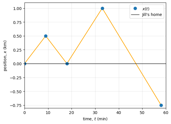
Jill sets out from her home to deliver flyers for her yard sale, traveling due east along her street lined with houses. At \(0.5\ {\rm km}\) and \(9\ {\rm min}\) later she runs out of flyers and has to retrace her steps back to her house to get more. This takes an additional \(9\ {\rm min}\). After picking up more flyers, she sets out again on the same path, continuing where she left off, and ends up \(1.0\ {\rm km}\) from her house. This third leg of her trip takes \(15\ {\rm min}\). At this point she turns back toward her house, heading west. After \(1.75\ {\rm km}\) and \(25\ {\rm min}\) she stops to rest.
a. What is Jill’s total displacement to the point where she stops to rest?
b. What is the magnitude of the final displacement?
c. What is the average velocity during her entire trip?
d. What is the total distance traveled?
e. Make a graph of position versus time.
The Model
Jill’s motion is one-dimensional along an east-west street. We choose east as the positive \(x\)-direction, west as the negative \(x\)-direction, and Jill’s home as the origin. The trip is broken into straight-line segments, so the net displacement depends only on the starting and ending positions, while the total distance depends on the length of every segment traveled.
The Math
We choose Jill’s home as \(x_o=0\) and reconstruct her position at the end of each leg. After the first leg, she is at \(x_1=+0.5\ {\rm km}\) after \(9\ {\rm min}\). After returning home, she is at \(x_2=0\) after \(18\ {\rm min}\). After the third leg, she is at \(x_3=+1.0\ {\rm km}\) after \(33\ {\rm min}\). During the final leg, Jill travels \(1.75\ {\rm km}\) west from \(x_3=+1.0\ {\rm km}\), so her final position is given by
The signed displacement during each segment is the change in position for that segment, which gives
(a) The total displacement is the change from the initial position to the final position, which is given by
(b) The magnitude of the final displacement is the absolute value of the total displacement, which is
(c) The total elapsed time is the sum of the four time intervals, which gives
The average velocity over the entire trip is the total displacement divided by the total elapsed time, which gives
(d) The total distance traveled is the sum of the magnitudes of the segment displacements, which gives
(e) The position-time graph is made from the positions at the end of each leg, so the plotted points are \((0\ {\rm min},0)\), \((9\ {\rm min},0.5\ {\rm km})\), \((18\ {\rm min},0)\), \((33\ {\rm min},1.0\ {\rm km})\), and \((58\ {\rm min},-0.75\ {\rm km})\).
The Conclusion
Jill’s final displacement is \(\boxed{-0.75\ {\rm km}}\), so she ends \(\boxed{0.75\ {\rm km}}\) west of her house. Her average velocity is \(\boxed{-0.013\ {\rm km/min}}\), where the negative sign shows that her net motion is westward. Her total distance traveled is \(\boxed{3.75\ {\rm km}}\), which is larger than the magnitude of her displacement because she reverses direction more than once.
The Verification
The Python cell below stores the time and position at the end of each leg, computes the total displacement, computes the average velocity, and sums the absolute segment displacements. The position-time graph is piecewise linear because the known data identify Jill’s position only at the endpoints of each segment.
import numpy as np
import matplotlib.pyplot as plt
# --- Data from the problem (time in min, position in km) ---
t = np.array([0, 9, 18, 33, 58])
x = np.array([0, 0.5, 0, 1.0, -0.75])
# Segment displacements and totals
dx = np.diff(x) #np.diff finds \Delta x
dt_total = t[-1] - t[0]
dx_total = x[-1] - x[0]
distance_total = np.sum(np.abs(dx))
v_avg = dx_total / dt_total
print(f"The total displacement for the trip is {dx_total:.2f} km.")
print(f"The magnitude of the total displacement is {abs(dx_total):.2f} km.")
print(f"The average velocity for the full trip is {v_avg:.4f} km/min.")
print(f"The total distance traveled during the trip is {distance_total:.2f} km.")
# --- Plot position vs time ---
fig = plt.figure()
ax = fig.add_subplot(111)
ax.plot(t, x, "-",color='orange')
ax.plot(t, x, '.', ms=15,label=r"$x(t)$")
ax.set_xlabel(r"time, $t$ (min)")
ax.set_ylabel(r"position, $x$ (km)")
ax.axhline(0, linewidth=1,color='k',label="Jill's home") # home reference line
ax.legend()
ax.grid(True, alpha=0.3)
# Tight limits to remove excess whitespace
ax.set_xlim(0,60)
ax.set_ylim(-0.8, 1.1)
plt.show()
The total displacement for the trip is -0.75 km.
The magnitude of the total displacement is 0.75 km.
The average velocity for the full trip is -0.0129 km/min.
The total distance traveled during the trip is 3.75 km.
3.2. Instantaneous Velocity and Speed#
This narration is AI-generated from the course text.
3.2.1. Instantaneous Velocity#
The quantity that tells us how fast an object is moving anywhere along its path is the instantaneous velocity, or simply velocity. It is the average velocity between two discrete points on the path.
Suppose we know the position \(x\) of an object at any time \(t\), then we would know the continuous function \(x(t)\). We can express the average velocity \(\bar{v}\) by
To find the instantaneous velocity at any position, we let \(t_1 \rightarrow t\) and \(t_2 \rightarrow t + \Delta t\). Then we substitute into our expression for the average velocity and define \(v(t)\) by,
We now define the instantaneous velocity of an object is the limit of the average velocity \(\bar{v}\) as the elapsed time \(\Delta t\) approaches zero, or the derivative of \(x\) with respect to \(t\):
Instantaneous velocity is a vector with dimension of \(L/T\). Since the definition of average velocity is written in terms of the change in position \(\Delta x\) over a specific time interval \(\Delta t\), we also refer to the velocity as the rate of change of the position function.
The rate of change is a measure of how fast a function is changing at a time \(t\), or the slope of the line that is tangent to the curve at \(t\). The displacement at the initial time \(t_o\) is zero (i.e., \(\Delta x = 0\)), therefore the velocity will also be zero and the slope will be flat.
Checkpoint
On a position-versus-time graph, what does a horizontal tangent line mean about the velocity at that instant?
At other times (\(t_1,\ t_2,\dots,\ t_N\)), the velocity is not zero (unless the position never changes) because the slope would be positive or negative. If the function \(x(t)\) had a minimum, then the slope would also be zero (i.e., \(v(t) = 0\)). Thus, the zeros of the velocity function give the minimum and maximum of the position function.
Fig. 3.1 In a graph of position versus time, the instantaneous velocity is the slope of the tangent line at a given point. Image Credit: OpenStax: Instantaneous Velocity and Speed.#
3.2.1.1. Example Problem: Plotting velocity from position#
Exercise 3.2
The Problem
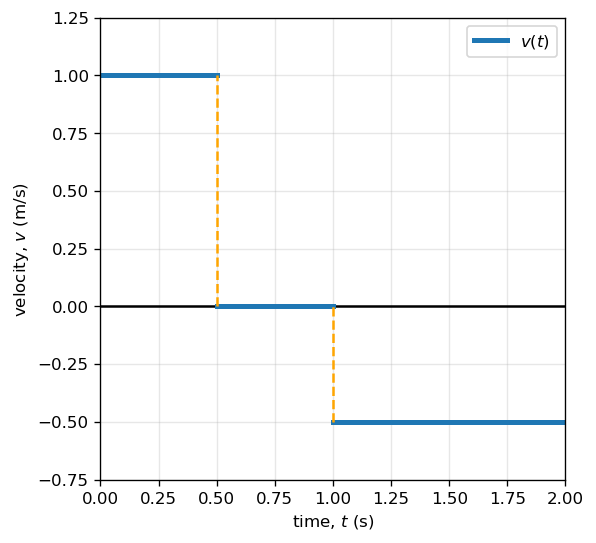
A position-versus-time graph is shown in Fig. 3.2. Using this graph, determine the corresponding velocity-versus-time graph.
Specifically:
Identify the velocity during each time interval.
Sketch or describe the resulting velocity-time graph.
Fig. 3.2 The object starts out in the positive direction, stops for a short time, and then reverses direction, heading back toward the origin. Image Credit: OpenStax: Instantaneous Velocity and Speed.#
The Model
The motion is one-dimensional along a straight line. The graph is made of straight-line position segments, so the velocity is constant within each time interval. A positive slope represents motion in the positive direction, a zero slope represents zero velocity, and a negative slope represents motion in the negative direction.
The Math
(a) The velocity during each interval is the slope of the position-versus-time graph. During the first interval, the position changes from \(0.0\ {\rm m}\) to \(0.5\ {\rm m}\) while the time changes from \(0.0\ {\rm s}\) to \(0.5\ {\rm s}\), which gives
During the second interval, the position remains fixed at \(0.5\ {\rm m}\) while the time changes from \(0.5\ {\rm s}\) to \(1.0\ {\rm s}\), which gives
During the third interval, the position changes from \(0.5\ {\rm m}\) to \(0.0\ {\rm m}\) while the time changes from \(1.0\ {\rm s}\) to \(2.0\ {\rm s}\), which gives
(b) The velocity-time graph is therefore piecewise constant, with horizontal segments at \(+1.0\ {\rm m/s}\), \(0.0\ {\rm m/s}\), and \(-0.5\ {\rm m/s}\) over the three corresponding intervals.
The Conclusion
The velocity is \(\boxed{+1.0\ {\rm m/s}}\) from \(0\) to \(0.5\ {\rm s}\), \(\boxed{0.0\ {\rm m/s}}\) from \(0.5\ {\rm s}\) to \(1.0\ {\rm s}\), and \(\boxed{-0.5\ {\rm m/s}}\) from \(1.0\ {\rm s}\) to \(2.0\ {\rm s}\). The signs match the physical interpretation of the graph: the object first moves in the positive direction, then stops, and finally moves back toward the origin.
The Verification
The Python cell below constructs the velocity-time graph from the three slopes found analytically. The horizontal pieces in the graph confirm that each straight-line segment of the position-time graph corresponds to a constant velocity over that interval.
import numpy as np
import matplotlib.pyplot as plt
# Time intervals (s)
t = np.array([0.0, 0.5, 1.0, 2.0])
# Corresponding velocities (m/s)
v = np.array([1.0, 0.0, -0.5])
fig = plt.figure(figsize=(5,5),dpi=120)
ax = fig.add_subplot(111)
ax.axhline(0, linewidth=1.5, color='k')
# Plot piecewise-constant velocity
ax.plot([0,0.5],[1,1],'-',color='tab:blue',lw=3,label=r"$v(t)$")
ax.plot([0.5,1.0],[0,0],'-',color='tab:blue',lw=3)
ax.plot([1,2],[-0.5,-0.5],'-',color='tab:blue',lw=3)
# Plot lines to connect the jumps; these are not physical
#axvline(x_o,y_o/y_range,y_f/y_range,kwargs); the y-values are scaled over the full y-range
ax.axvline(0.5,0.375,0.875,linestyle='--',color='orange',lw=1.5)
ax.axvline(1.0,0.125,0.375,linestyle='--',color='orange',lw=1.5)
ax.set_xlabel(r"time, $t$ (s)")
ax.set_ylabel(r"velocity, $v$ (m/s)")
ax.legend()
ax.grid(True, alpha=0.3)
# Tight limits
ax.set_xlim(0, 2.0)
ax.set_ylim(-0.75, 1.25)
plt.show()
3.2.2. Speed#
Most people use the terms speed and velocity interchangeably. In physics, they do not have the same meaning and are distinct concepts. Speed is a scalar, while velocity is a vector.
We calculate the average speed \(\bar{s}\) by
Average speed is different than average velocity because the numerator Total distance is always a positive quantity, and hence, average speed cannot be negative. For example, if a trip starts and ends at the same location,
the total displacement is zero, which implies the average velocity is zero.
the total distance traveled is not zero and thus, the average speed is not zero.
However, we can calculate the instantaneous speed from the magnitude of the instantaneous velocity, or
Checkpoint
A particle has velocity \(v = -6\ {\rm m/s}\).
What is its speed?
Two particles moving in opposite directions can have the same speed, but have different velocities. Table 3.1 shows some typical speeds in \(\rm m/s\) and \(\rm mph\).
Speed |
m/s |
mi/h |
|---|---|---|
Continental drift |
\(10^{-7}\) |
\(2\times10^{-7}\) |
Brisk walk |
1.7 |
3.9 |
Cyclist |
4.4 |
10 |
Sprint runner |
12.2 |
27 |
Rural speed limit |
24.6 |
56 |
Official land speed record |
341.1 |
763 |
Speed of sound at sea level |
343 |
768 |
Space shuttle on reentry |
7,800 |
17,500 |
Escape velocity of Earth\(^\ast\) |
11,200 |
25,000 |
Orbital speed of Earth around the Sun |
29,783 |
66,623 |
Speed of light in a vacuum |
299,792,458 |
670,616,629 |
\(^\ast\) Escape velocity is the speed at which an object must be launched so that it overcomes Earth’s gravity and is not pulled back toward Earth.
3.2.3. Calculating Instantaneous Velocity#
If the position function \(x(t)\) is has the form of \(at^n\), where \(A\) is a constant and \(n\) is an integer, then it can be differentiated using the power rule by,
Note
If there are additional terms added together (e.g., \(x(t) = At^n + Bt^m\)), then the power rule of differentiation is distributive, where it can be done multiple times and the solution is the sum of those terms.
If \(x(t) = A\), then the derivative is equal to zero. The slope of a constant horizontal line is zero like we saw at the maximum \(x(t_o)\) in Fig. 3.1.
3.2.3.1. Example Problem: Instantaneous Velocity vs. Average Velocity#
Exercise 3.3
The Problem
The position of a particle moving along the \(x\)-axis is given by
\[ x(t) = (3.0\ {\rm m/s})t + (0.5\ {\rm m/s^3})t^3.\]a. Using the definition of instantaneous velocity, find the instantaneous velocity at \(t = 2.0\ {\rm s}\).
b. Calculate the average velocity between \(t = 1.0\ {\rm s}\) and \(t = 3.0\ {\rm s}\).
The Model
The particle moves along the \(x\)-axis, so its motion is one-dimensional. Instantaneous velocity describes the rate at which the position changes at a single instant, while average velocity describes the net change in position over a finite time interval. Because the position function is a polynomial in time, the instantaneous velocity can be found by differentiating the position function directly.
The Math
(a) The instantaneous velocity is the derivative of the position function with respect to time, which gives
The instantaneous velocity at \(t=2.0\ {\rm s}\) is found by evaluating this function at that time, which gives
(b) The average velocity between \(t_1=1.0\ {\rm s}\) and \(t_2=3.0\ {\rm s}\) requires the position at each endpoint, which gives
The average velocity is the displacement over the elapsed time, which gives
The Conclusion
The instantaneous velocity at \(t=2.0\ {\rm s}\) is \(\boxed{9.0\ {\rm m/s}}\), and the average velocity from \(1.0\ {\rm s}\) to \(3.0\ {\rm s}\) is \(\boxed{9.5\ {\rm m/s}}\). These values are close but not identical because the velocity is changing over the interval.
The Verification
The Python cell below evaluates the analytical velocity function at \(t=2.0\ {\rm s}\) and computes the average velocity from the two endpoint positions. These calculations mirror the derivative and slope methods used in the analytical solution.
import numpy as np
import matplotlib.pyplot as plt
# Position and velocity functions (from the analytic work)
def x(t):
return 3.0*t + 0.5*t**3
def v(t):
return 3.0 + 1.5*t**2
# Quantities requested in the problem
v_inst = v(2.0)
v_avg = (x(3.0) - x(1.0)) / (3.0 - 1.0)
print(f"The instantaneous velocity at t = 2.0 s is {v_inst:.1f} m/s.")
print(f"The average velocity from t = 1.0 s to t = 3.0 s is {v_avg:.1f} m/s.")
The instantaneous velocity at t = 2.0 s is 9.0 m/s.
The average velocity from t = 1.0 s to t = 3.0 s is 9.5 m/s.
3.3. Average and Instantaneous Acceleration#
This narration is AI-generated from the course text.
3.3.1. Average Acceleration#
The average acceleration \(\bar{a}\) is the rate of change for the velocity \(v\):
where \(t\) is time.
The SI units for acceleration are meters per second squared (or meters per second per second) and abbreviated as \(\rm m/s^2\). This means how much the velocity has changed every second, where the velocity can change in either magnitude or direction due to it being a vector. For example,
a runner traveling at \(10\ {\rm km/h}\) due east slows to a stop reverses direction, and continues to run \(10\ {\rm km/h}\) due west.
Before turning around, the runner had one average acceleration, then a different average acceleration afterwards. This is shown mathematically as,
The magnitude of the velocity is the same in both directions, however the direction is different. Acceleration is a vector in the same direction as the change in velocity \(\Delta v\). Acceleration is a change in speed or direction, or both.
Note
Although acceleration is in the direction of the change in velocity, it is not always in the direction of motion. When an object slows down, its acceleration is opposite to the direction of its motion.
The term deceleration can cause confusion because it is not a vector and it does not point to a specific direction with respect to a specific direction.
We can say the runner was decelerating before coming to a stop and accelerating afterward, but we shouldn’t include the coordinate system unit vector (\(\hat{i}\) or \(-\hat{i}\)) in our analysis. Otherwise the runner always has a negative acceleration, in contrast to our intuition. Instead of using the term deceleration, we describe the motion more accurately with a positive or negative acceleration relative to the coordinate system.
If an object has a velocity in the positive direction with respect to the origin and it acquires a constant negative acceleration, the object eventually comes to rest and reverses direction (i.e., our runner in \(\Delta t_1\)). Eventually, the object passes through the origin going in the opposite direction (i.e., our runner in \(\Delta t_2\)).
Checkpoint
An object has \(v = +8\ {\rm m/s}\) and \(a = -2\ {\rm m/s^2}\).
Is it moving in the positive or negative direction? Is it speeding up or slowing down?
The sign of acceleration tells us the direction of the change in velocity, not whether the object is speeding up or slowing down. To decide whether the speed is increasing or decreasing, we compare the signs of velocity and acceleration. If \(v\) and \(a\) have the same sign, the object speeds up. If \(v\) and \(a\) have opposite signs, the object slows down.
Situation |
Sign of \(v\) |
Sign of \(a\) |
What happens to the speed? |
|---|---|---|---|
Moving in the positive direction and speeding up |
\(+\) |
\(+\) |
Speed increases |
Moving in the positive direction and slowing down |
\(+\) |
\(-\) |
Speed decreases |
Moving in the negative direction and speeding up |
\(-\) |
\(-\) |
Speed increases |
Moving in the negative direction and slowing down |
\(-\) |
\(+\) |
Speed decreases |
Fig. 3.3 An object in motion with a velocity vector toward the east under negative acceleration comes to a rest and reverses direction. It passes the origin going in the opposite direction after a long enough time. Image Credit: OpenStax: Average and Instantaneous Acceleration.#
3.3.1.1. Example Problem: Racehorse Leaves the Gate#
Exercise 3.4
The Problem
A racehorse coming out of the gate accelerates from rest to a velocity of \(15.0 {\rm m/s}\) due west in \(1.80 {\rm s}\). What is its average acceleration?
Fig. 3.4 Identify the coordinate system, the given information, and what you want to determine. Image Credit: OpenStax: Average and Instantaneous Acceleration.#
The Model
The horse moves in one dimension along an east-west line. We choose east as the positive direction and west as the negative direction. Since the horse starts from rest and ends with a westward velocity, the change in velocity is directed west, so the average acceleration should be negative in this coordinate system.
The Math
The average acceleration is the change in velocity divided by the elapsed time, which is given by
The horse starts from rest and west is the negative direction, so the initial and final velocities are \(v_o=0\) and \(v_f=-15.0\ {\rm m/s}\). The change in velocity is therefore
Dividing this change in velocity by the elapsed time gives the average acceleration as
The Conclusion
The horse’s average acceleration is \(\boxed{-8.33\ {\rm m/s^2}}\). The negative sign means the acceleration points west, which is consistent with the horse increasing its speed westward from rest.
The Verification
The Python cell below computes the change in velocity and divides by the elapsed time. This mirrors the analytical definition of average acceleration and confirms the westward acceleration.
# Given values
v0 = 0.0 # m/s
vf = -15.0 # m/s (west is negative)
dt = 1.80 # s
# Average acceleration
a_avg = (vf - v0) / dt
print(f"The racehorse's average acceleration is {a_avg:.2f} m/s^2.")
The racehorse's average acceleration is -8.33 m/s^2.
3.3.2. Instantaneous Acceleration#
Instantaneous acceleration \(a\), or acceleration at a time \(t\), is found using the same process discussed for instantaneous velocity. We calculate, the average acceleration between two points in time \(\Delta t\) and let \(\Delta t \rightarrow 0\). The result is the derivative of the velocity function \(v(t)\) and is expressed as
We can show that the instantaneous acceleration at \(t_o\) is the slope of the tangent line to the velocity graph at time \(t_o\). The average acceleration approaches the instantaneous acceleration as \(\Delta t \rightarrow 0\).
Checkpoint
On a velocity-versus-time graph, what does a horizontal tangent line mean about the acceleration at that instant?
Fig. 3.5 In a graph of velocity versus time, instantaneous acceleration is the slope of the tangent line. Image Credit: OpenStax: Average and Instantaneous Acceleration.#
As shown in Fig. 3.5a, the velocity has a maximum when its slope is zero, which corresponds to a zero of the acceleration function. In Fig. 3.5b, there is a minimum velocity when the acceleration is zero. The zeros of the acceleration function give either the minimum or maximum velocity.
Calculus Note: Derivatives, Extrema, and Evolution
Finding Extrema by Setting the Derivative to Zero
One of the most powerful and general uses of calculus is identifying where a quantity reaches a maximum or minimum.
Given a function \(f(x)\), extrema occur at critical points, which satisfy
(or where the derivative is undefined).
This works because the derivative represents the rate of change of the function. At a maximum or minimum, the function momentarily stops increasing or decreasing, so its slope is zero.
Examples
In kinematics, setting \(v(t) = \frac{dx}{dt} = 0\) finds when an object momentarily stops or turns around.
In optimization, setting \(\frac{dE}{dx} = 0\) finds stable equilibrium configurations.
In thermodynamics, extrema of entropy or energy determine equilibrium states.
This method applies to any differentiable function, not just position or velocity.
Using Derivatives to Evolve a System
Derivatives do more than identify special points. They describe how systems change in time. Many physical laws are written as differential equations, which specify how a quantity evolves:
Here, the derivative tells us how the system changes at each instant. Solving the differential equation allows us to predict the system’s future behavior.
Examples
Newton’s Second Law:
\[ m\frac{dv}{dt} = F(x,v,t) \]determines how velocity evolves from forces.
Radioactive decay:
\[ \frac{dN}{dt} = -\lambda N \]describes how a quantity decreases over time.
Population growth, electrical circuits, orbital motion, and climate models are all governed by differential equations.
Big Picture
Setting derivatives equal to zero finds where something stops changing (extrema, turning points, equilibrium).
Using derivatives in equations tells us how something changes (motion, growth, decay, evolution).
Together, these ideas form the mathematical backbone of physics, engineering, and applied science.
3.3.2.1. Example Problem: Calculating Instantaneous Acceleration#
Exercise 3.5
The Problem
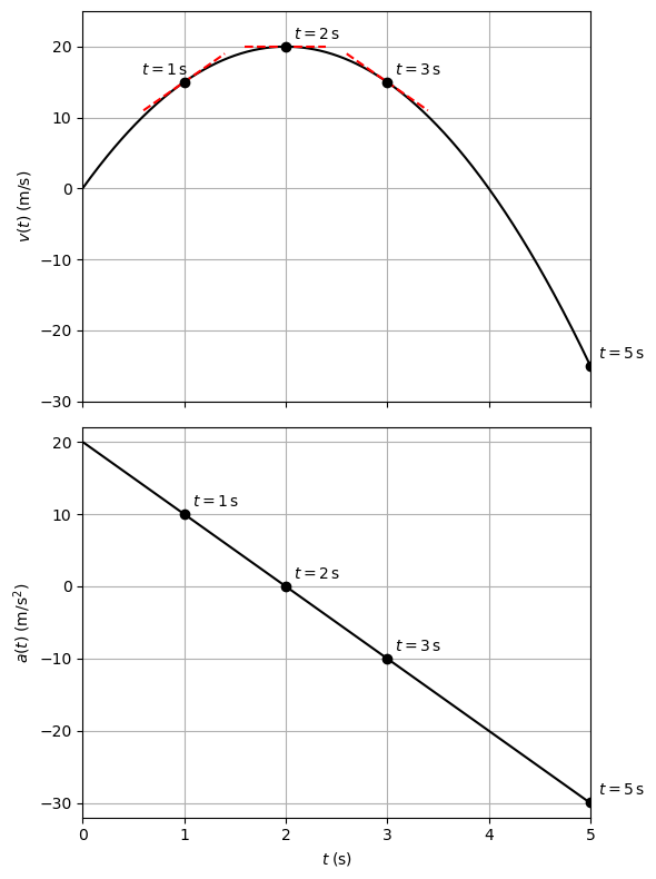
A particle is in one-dimensional motion and is accelerating. The functional form of its velocity is \(v(t) = (20\ {\rm m/s^2})t - (5\ {\rm m/s^3})t^2\).
a. Find the functional form of the acceleration.
b. Find the instantaneous velocity at \(t = 1,\ 2,\ 3,\) and \(5\ {\rm s}\).
c. Find the instantaneous acceleration at \(t = 1,\ 2,\ 3,\) and \(5\ {\rm s}\).
d. Interpret the results of part (c) in terms of the directions of the acceleration and velocity vectors.
The Model
The particle moves in one dimension, so the signs of velocity and acceleration represent direction. Acceleration describes the time rate of change of velocity. If velocity and acceleration have the same sign, the particle speeds up; if they have opposite signs, the particle slows down.
The Math
(a) The acceleration function is found by differentiating the velocity function with respect to time, which gives
(b) The instantaneous velocity values are found by evaluating the velocity function at each requested time, which gives
(c) The instantaneous acceleration values are found by evaluating the acceleration function at each requested time, which gives
(d) At \(t=1\ {\rm s}\), both velocity and acceleration are positive, so the particle is moving in the positive direction and speeding up. At \(t=2\ {\rm s}\), the velocity is positive and the acceleration is zero, so the velocity is momentarily at its maximum value. At \(t=3\ {\rm s}\), the velocity is positive but the acceleration is negative, so the particle is slowing down. At \(t=5\ {\rm s}\), both velocity and acceleration are negative, so the particle is moving in the negative direction and speeding up.
The Conclusion
The acceleration function is \(\boxed{a(t)=20\ {\rm m/s^2}-(10\ {\rm m/s^3})t}\). The requested velocity values are \(\boxed{15\ {\rm m/s}}\), \(\boxed{20\ {\rm m/s}}\), \(\boxed{15\ {\rm m/s}}\), and \(\boxed{-25\ {\rm m/s}}\). The corresponding acceleration values are \(\boxed{10\ {\rm m/s^2}}\), \(\boxed{0\ {\rm m/s^2}}\), \(\boxed{-10\ {\rm m/s^2}}\), and \(\boxed{-30\ {\rm m/s^2}}\), which show when the particle speeds up, slows down, or reverses direction.
The Verification
The Python cell below evaluates the analytical velocity and acceleration functions at the requested times. The plotted functions confirm that the velocity reaches its maximum when the acceleration crosses zero.
Show code cell source
import numpy as np
import matplotlib.pyplot as plt
# Analytic functions (for comparison)
def v_analytic(t):
return 20*t - 5*t**2
def a_analytic(t):
return 20 - 10*t
# Time grid (uniform spacing is explicit)
dt = 0.01
t = np.arange(0, 5.01, dt)
# Sample velocity from the analytic function (this is our "measured" data stream)
v = v_analytic(t)
# Central-difference acceleration from sampled velocity (independent numerical verification)
# a_i ≈ (v_{i+1} - v_{i-1}) / (2 dt)
a_num = np.empty_like(v)
a_num[1:-1] = (v[2:] - v[:-2]) / (2*dt)
# One-sided differences at endpoints (not central, but avoids NaNs at the plot edges)
a_num[0] = (v[1] - v[0]) / dt
a_num[-1] = (v[-1] - v[-2]) / dt
# Times for annotations / tangents
t_points = np.array([1, 2, 3, 5])
t_tangent = np.array([1, 2, 3])
# Helper: find nearest index on the grid
def idx_of_time(tp):
return int(np.round((tp - t[0]) / dt))
# Print comparisons at the marked times
print("Instantaneous values (analytic vs. numeric central-difference):")
for tp in t_points:
i = idx_of_time(tp)
print(
f"At t = {tp:.0f} s, the velocity is {v[i]:.2f} m/s, "
f"the analytical acceleration is {a_analytic(tp):.2f} m/s^2, "
f"and the numerical acceleration is {a_num[i]:.2f} m/s^2."
)
# Plot settings packed for reuse in a single loop
series = [
{"y": v,"color": "black","ylabel": r"$v(t)\;(\mathrm{m/s})$","ylim": (-30, 25),"use_tangents": True},
{"y": a_num,"color": "black","ylabel": r"$a(t)\;(\mathrm{m/s^2})$", "ylim": (-32, 22),"use_tangents": False},
]
fig, axes = plt.subplots(nrows=2, ncols=1, figsize=(6, 8), sharex=True,dpi=100)
for ax, s in zip(axes, series):
y = s["y"]
# Main curve and marked points
ax.plot(t, y, color=s["color"])
ax.scatter(t_points, [y[idx_of_time(tp)] for tp in t_points], color="black", zorder=3)
# Annotations
for tp in t_points:
i = idx_of_time(tp)
t_off = t[i]
if abs(tp - 1)<1e-4 and s["use_tangents"]:
t_off += -0.5
ax.annotate(rf"$t={tp}\,\mathrm{{s}}$",(t_off, y[i]),textcoords="offset points",xytext=(5, 5),fontsize=10)
# Tangent lines on v(t) panel: slope comes from *numeric* acceleration at that time
# (this reinforces "slope = derivative" using the numerical derivative)
if s["use_tangents"]:
half_span = 0.4
for tp in t_tangent:
i0 = idx_of_time(tp)
slope = a_num[i0] # numeric slope
t0,v0 = t[i0],y[i0]
t_local = np.arange(t0 - half_span, t0 + half_span + dt, dt)
v_tan = v0 + slope * (t_local - t0)
ax.plot(t_local, v_tan, linestyle="--", color="r", linewidth=1.5)
ax.set_ylabel(s["ylabel"])
ax.set_xlim(0, 5)
ax.set_ylim(*s["ylim"])
ax.grid(True)
axes[1].set_xlabel(r"$t\;(\mathrm{s})$")
plt.tight_layout()
plt.show()
Instantaneous values (analytic vs. numeric central-difference):
At t = 1 s, the velocity is 15.00 m/s, the analytical acceleration is 10.00 m/s^2, and the numerical acceleration is 10.00 m/s^2.
At t = 2 s, the velocity is 20.00 m/s, the analytical acceleration is 0.00 m/s^2, and the numerical acceleration is 0.00 m/s^2.
At t = 3 s, the velocity is 15.00 m/s, the analytical acceleration is -10.00 m/s^2, and the numerical acceleration is -10.00 m/s^2.
At t = 5 s, the velocity is -25.00 m/s, the analytical acceleration is -30.00 m/s^2, and the numerical acceleration is -29.95 m/s^2.
3.3.3. Getting a Feel for Accelerations#
You feel an acceleration when riding an elevator or stepping on the gas (“go”) pedal in your car. However, the sense of scale for acceleration is provided in Table 3.3. Expressing acceleration in units of \(g\) helps relate these values to everyday experience and to the forces objects must withstand.
Acceleration |
Value (m/s²) |
Value (\(g\)) |
|---|---|---|
High-speed train |
0.25 |
0.03 |
Elevator |
2 |
0.20 |
Cheetah |
5 |
0.5 |
Object in free fall without air resistance near the surface of Earth, \(g\) |
9.8 |
1 |
Space shuttle maximum during launch |
29 |
3 |
Parachutist peak during normal opening of parachute |
59 |
6 |
F16 aircraft pulling out of a dive |
79 |
8 |
Explosive seat ejection from aircraft |
147 |
15 |
Sprint missile |
982 |
100 |
Fastest rocket sled peak acceleration |
1540 |
160 |
Jumping flea |
3200 |
330 |
Baseball struck by a bat |
30,000 |
3,000 |
Closing jaws of a trap-jaw ant |
1,000,000 |
100,000 |
Proton in the Large Hadron Collider |
\(2 \times 10^{9}\) |
\(2 \times 10^{8}\) |
3.4. Motion with Constant Acceleration#
This narration is AI-generated from the course text.
Before using the constant-acceleration equations, we need to decide whether this model applies. These equations are powerful, but they only describe motion where the acceleration is constant over the interval being analyzed.
Checkpoint
A car accelerates from rest, then later brakes to a stop.
Should the entire trip be modeled with one constant acceleration, or should it be split into separate intervals?
Choosing a One-Dimensional Motion Model
Use the following questions before choosing an equation.
Is the motion along one straight axis?
If yes, the motion can be described with one-dimensional position, velocity, and acceleration.Is the acceleration constant over the interval?
If yes, the constant-acceleration equations can be used. If no, use graphs, calculus, or split the motion into intervals where the acceleration is approximately constant.Are the known and unknown quantities among \(x\), \(x_o\), \(v\), \(v_o\), \(a\), and \(t\)?
If yes, choose an equation that contains the unknown and the given quantities.Does the sign of the answer make physical sense?
Check whether the object is moving in the expected direction, speeding up or slowing down appropriately, and whether any time value is physically meaningful.
3.4.1. Notation#
To make things simpler, we introduce some conventions in notation. One simplification is taking \(t_o = 0\), which is the point in time when you begin to measure. Time exists before this point, but until “you get your Delorean to 88 mph”, then it doesn’t make sense to include the past.
The elapsed time goes from \(\Delta t = t_f - t_o\) to \(\Delta t = t_f\). We don’t need the subscript \(f\) anymore. So, the elapsed time is \(\Delta t = t\). We can drop the subscript \(f\) from the \(\Delta x\) and \(\Delta v\) as well. In our simplified notation we have
where the subscript \(o\) denotes an initial value and the absence of a subscript indicates the final value of the variable.
For now, we will also make the assumption that the acceleration is constant. As a result, the average and instantaneous acceleration are equal, or
In many situations in this course, the acceleration is constant. When it isn’t (e.g., a car accelerating to top speed, then braking to a stop), the motion will be considered in separate parts (like with the runner) and each part has its own constant acceleration.
3.4.2. Displacement and Position from Velocity#
To get our first two equations, we start with the definition of average velocity:
and substitute the simplified notation to get
Solving for \(x\) gives
where the arithmetic average velocity is
This version of \(\bar{v}\) reflects that when acceleration is constant, then \(\bar{v}\) is the simple average of the initial and final velocities.
3.4.3. Solving for Final Velocity from Acceleration and Time#
We can derive another useful equation by manipulating the definition of acceleration:
By substituting the simplified notation for \(\Delta v\) and \(\Delta t\), we have
Solving for \(v\) yields
The above equation gives us insight into relationships among velocity, acceleration, and time. We can see that
Final velocity depends on both acceleration and time
For zero acceleration, then the initial and final velocities are equal (i.e., \(v=v_o\))
If \(a<0\), then \(v<v_o\).
These relationships fit our intuition, which can be a good sign.
3.4.3.1. Example Problem: Calculating Final Velocity#
Exercise 3.6
The Problem
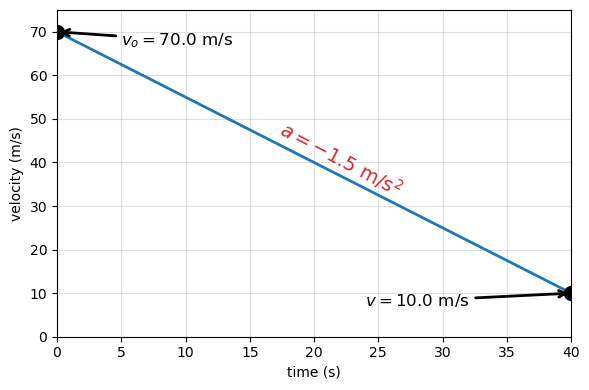
An airplane lands with an initial velocity of \(70.0\ {\rm m/s}\) and then accelerates opposite to the motion at \(1.50\ {\rm m/s^2}\) for \(40.0\ {\rm s}\). What is its final velocity?
Fig. 3.6 The airplane lands with an initial velocity of \(70.0\ {\rm m/s}\) and slows to a final velocity of \(10.0\ {\rm m/s}\) before heading for the terminal. Note the acceleration is negative because its direction is opposite to its velocity, which is positive. Figure Credit: OpenStax: Motion with Constant Acceleration.#
The Model
The airplane moves in one dimension with constant acceleration. We choose the initial direction of motion as positive. Since the acceleration is opposite the motion, the acceleration is negative in this coordinate system.
The Math
For constant acceleration, the final velocity is related to the initial velocity, acceleration, and elapsed time by
The acceleration is negative because it points opposite the positive direction of motion, so the velocity-time relation gives
The Conclusion
The airplane’s final velocity is \(\boxed{10.0\ {\rm m/s}}\). The result is still positive, so the airplane is still moving in its original direction after \(40.0\ {\rm s}\), but it has slowed substantially.
The Verification
The Python cell below evaluates the same velocity-time relation used in the analytical solution. The velocity-time graph confirms that constant negative acceleration decreases the velocity linearly from \(70.0\ {\rm m/s}\) to \(10.0\ {\rm m/s}\).
import numpy as np
import matplotlib.pyplot as plt
# Given values
v0 = 70.0 # initial velocity (m/s)
a = -1.50 # acceleration (m/s^2)
t_final = 40.0 # time (s)
# Compute final velocity
v_final = v0 + a * t_final
print(f"After {t_final:.0f} s, the airplane's final velocity is {v_final:.1f} m/s.")
#-----
# Time array (uniform spacing, intentional)
dt = 0.1
t = np.arange(0, t_final + dt, dt)
# Velocity as a function of time
v = v0 + a * t
# Create the figure using object-oriented style
fig = plt.figure(figsize=(6, 4),dpi=100)
ax = fig.add_subplot(111)
ax.plot(t, v, linewidth=2)
ax.plot([0, t_final], [v0, v_final],'ko',ms=10,zorder=3)
# Labels and limits
ax.set_xlabel("time (s)")
ax.set_ylabel("velocity (m/s)")
ax.set_xlim(0, t_final)
ax.set_ylim(0, v0 + 5)
# Annotations instead of titles
ax.annotate(rf"$v_o = {v0:.1f}\ \mathrm{{m/s}}$",xy=(0, v0), fontsize=12,
xytext=(5, v0 - 3),arrowprops=dict(arrowstyle="->",linewidth=2))
ax.annotate(rf"$v = {v_final:.1f}\ \mathrm{{m/s}}$",xy=(t_final, v_final), fontsize=12,
xytext=(t_final - 16, v_final - 3),arrowprops=dict(arrowstyle="->",linewidth=2))
ax.text(17,32,rf"$a= {a:.1f}\ \mathrm{{m/s^2}}$",rotation=-28,color='tab:red',fontsize=14)
ax.grid(True,alpha=0.4)
plt.tight_layout()
plt.show()
After 40 s, the airplane's final velocity is 10.0 m/s.
3.4.4. Solving for Final Position with Constant Acceleration#
We can use the equation that defines the average velocity \(\bar{v}\) that is related to time and displacement \(\Delta x\) with the arithmetic definition of average velocity. This gives us 3 equations as
where \(a\) is a constant acceleration and using our simplified notation. The third equation can be substituted into the second equation to get
Now we substitute this expression for \(\bar{v}\) into the equation for displacement yielding
The position equation can also be written using the final velocity instead of the initial velocity. This form is useful when \(v\), \(a\), and \(t\) are known, but \(v_o\) is not needed.
The velocity equation can be solved for the initial velocity, which gives
The position equation can then be rewritten by replacing \(v_o\) with \(v-at\), which gives
Expanding and combining the acceleration terms gives the equivalent position equation
Writing this result in displacement form gives
This equation describes the same constant-acceleration motion, but it is written in terms of the final velocity \(v\) rather than the initial velocity \(v_o\).
We can see the following relationships from the above equation:
Displacement depends on the time squared, when the acceleration is not zero.
The form of the equation is a quadratic, where it should plot as a parabola.
If the acceleration is zero, then it reduces to \(x = x_o + v_o t\). the equation for displacement under constant velocity \(v_o\).
3.4.4.1. Example Problem: Calculating Displacement of an Accelerating Object#
Exercise 3.7
The Problem
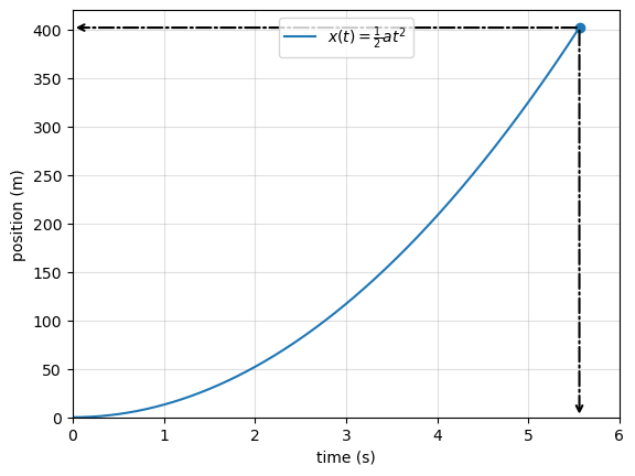
Dragsters can achieve an average acceleration of \(26.0\ {\rm m/s^2}\). Suppose a dragster accelerates from rest at this rate for \(5.56\ {\rm s}\). How far does it travel in this time?
Fig. 3.7 Sketch of an accelerating dragster. Figure Credit: OpenStax: Motion with Constant Acceleration.#
The Model
The dragster is modeled as a particle moving in one dimension with constant acceleration. It starts from rest at the starting line, which we choose as the origin. With these choices, the displacement is determined by the acceleration and the elapsed time.
The Math
For one-dimensional motion with constant acceleration, the position is given by
Because the dragster starts from rest at the origin, \(v_o=0\) and \(x_o=0\), so the position equation reduces to
The displacement after \(5.56\ {\rm s}\) is found by evaluating this expression, which gives
The Conclusion
The dragster travels \(\boxed{402\ {\rm m}}\) while accelerating from rest for \(5.56\ {\rm s}\). The large displacement over a short time is physically reasonable because the acceleration is very large.
The Verification
The Python cell below computes the position as a function of time using the same constant-acceleration model. Evaluating the final point and plotting the position-time curve confirm that the displacement grows quadratically and reaches approximately \(402\ {\rm m}\).
# Verification of displacement for constant acceleration
import numpy as np
import matplotlib.pyplot as plt
# Given values
a = 26.0 # acceleration (m/s^2)
t_final = 5.56 # final time (s)
# Time array (use arange for intentional spacing)
dt = 0.01
t = np.arange(0, t_final + dt, dt)
# Position as a function of time (x0 = 0, v0 = 0)
x = 0.5 * a * t**2
# Print final displacement
print(f"After {t_final:.2f} s, the dragster's displacement is {x[-1]:.0f} m.")
# Plot position vs time
fig, ax = plt.subplots()
ax.plot(t, x, label=r"$x(t)=\frac{1}{2}at^2$")
ax.scatter(t_final, x[-1], zorder=3)
# Arrows from endpoint to axes
ax.annotate("", xy=(t_final, 0), xytext=(t_final, x[-1]),
arrowprops=dict(arrowstyle="->", lw=1.5,ls='-.'))
ax.annotate("", xy=(0, x[-1]), xytext=(t_final, x[-1]),
arrowprops=dict(arrowstyle="->", lw=1.5,ls='-.'))
ax.set_xlabel("time (s)")
ax.set_ylabel("position (m)")
ax.legend(loc='upper center')
ax.set_xlim(0,6)
ax.set_ylim(0,420)
ax.grid(True,alpha=0.4)
plt.show()
After 5.56 s, the dragster's displacement is 402 m.
3.4.5. Solving for Final Velocity from Distance and Acceleration#
Since the acceleration \(a\) is constant, we can instead solve for the time \(t\) and substitute into the equation for displacement. We have the following equations:
Substituting the first and second equations into the final equation (and performing some algebra) gives
Solving for \(v^2\), we get
Formatting Grouped Expressions
When fractions, powers, or stacked expressions get tall, ordinary parentheses or brackets can look too small.
LaTeX can automatically resize delimiters using \left and \right.
Automatic resizing with \left( \right)
Use these when the contents are tall (fractions, exponents, roots):
\(\left(\frac{1}{2}at^2\right)\)
\(\left(\frac{x_2-x_1}{t_2-t_1}\right)\)
\(\left(a+\frac{b}{c}\right)^2\)
LaTeX adjusts the size of the parentheses to match the height of the expression inside.
Automatic resizing with \left[ \right]
Brackets behave the same way and are often clearer for long expressions:
\(\left[\frac{x_2-x_1}{t_2-t_1}\right]\)
\(\left[\frac{1}{2}at^2\right]_{t=0}^{t=t_f}\)
\(\left[a+\left(\frac{b}{c}\right)^2\right]\)
Mixing delimiter types
You can mix parentheses and brackets to improve readability:
\(\left[\frac{(x_2-x_1)}{(t_2-t_1)}\right]\)
\(\left(a+\frac{b}{c}\right)\left(a-\frac{b}{c}\right)\)
Suppressing one side
If you only want one visible delimiter, use a period . on the other side:
\(\left.\frac{dx}{dt}\right|_{t=2\ {\rm s}}\)
\(\left[\frac{1}{2}at^2\right.\)
Rule of thumb
Use ordinary
( )or[ ]for simple expressions.Use
\left( \right)or\left[ \right]whenever the expression contains fractions, roots, or stacked exponents.
This keeps your math clean, readable, and professional, especially in physics derivations.
Difference of Squares Identity
A very common algebra identity is
You can see it by distributing (or using FOIL to save a step):
This is useful for quickly simplifying expressions and for factoring quadratics that look like a difference of squares.
We can see the following relationships in this equation:
The final velocity depends on the acceleration and total displacement.
For a fixed acceleration, the stopping distance \((x-x_o)\) increases with the square of the velocity. It takes much farther to stop. This is shown by
\[ x-x_o = \frac{v_o^2}{2a} \propto v_o^2.\]
3.4.5.1. Example Problem: Calculating Final Velocity#
Exercise 3.8
The Problem
A dragster starts from rest and accelerates at an average rate of \(a=26.0\ {\rm m/s^2}\). In the previous example, it traveled a displacement of \(\Delta x = x-x_o = 402\ {\rm m}\).
Use a kinematic equation that does not involve time to find the dragster’s final velocity.
The Model
The dragster moves in one dimension with constant acceleration. It starts from rest and moves in the positive direction. Since the elapsed time is not needed, we use the time-independent relationship between speed, acceleration, and displacement.
The Math
For constant acceleration, the time-independent kinematic equation is
Because the dragster starts from rest, \(v_o=0\), and because the displacement is \(\Delta x=x-x_o\), the time-independent equation becomes
The final speed is the positive square root because the dragster accelerates forward, which gives
The Conclusion
The dragster’s final velocity is \(\boxed{145\ {\rm m/s}}\) in the forward direction. The positive root is selected because the dragster starts from rest and accelerates forward.
The Verification
The Python cell below computes the final speed from the same time-independent kinematic equation. It also checks consistency by using the displacement equation to recover the time and confirming that \(v=at\) gives the same final speed.
import numpy as np
# Given values
a = 26.0 # m/s^2
dx = 402.0 # m
# Time-free kinematics: v^2 = v0^2 + 2 a dx, with v0 = 0
v = np.sqrt(2 * a * dx)
# Unit conversions
v_kmh = v * 3.6
v_mph = v * 2.2369362920544
# Optional consistency check using dx = (1/2) a t^2 (valid because v0 = 0)
t = np.sqrt(2 * dx / a)
v_check = a * t
print(f"The final velocity found from distance and acceleration is {v:.1f} m/s.")
print(f"The same final velocity is {v_kmh:.1f} km/h.")
print(f"The same final velocity is {v_mph:.1f} mi/h.")
print(f"The consistency check gives a travel time of {t:.3f} s.")
print(f"The consistency check gives a final velocity of {v_check:.3f} m/s.")
print(f"The difference between the two final-velocity calculations is {abs(v_check - v):.3e} m/s.")
The final velocity found from distance and acceleration is 144.6 m/s.
The same final velocity is 520.5 km/h.
The same final velocity is 323.4 mi/h.
The consistency check gives a travel time of 5.561 s.
The consistency check gives a final velocity of 144.582 m/s.
The difference between the two final-velocity calculations is 0.000e+00 m/s.
3.4.6. Putting Equations Together#
Here’s a summary of the equations that we’ve developed thus far (under the assumption of constant \(a\)):
The equation we choose depends on which quantity is missing from the problem. The table below is useful only when the acceleration is constant over the interval being analyzed.
Equation |
Missing quantity |
Use this equation when… |
|---|---|---|
\(v = v_o + at\) |
\(x - x_o\) |
The displacement is not given and is not requested. |
\(x = x_o + v_ot + \frac{1}{2}at^2\) |
\(v\) |
The final velocity is not given and is not requested. |
\(v^2 = v_o^2 + 2a(x - x_o)\) |
\(t\) |
The time interval is not given and is not requested. |
\(x = x_o + \frac{1}{2}(v_o + v)t\) |
\(a\) |
The acceleration is not given and is not requested. |
\(x = x_o + vt - \frac{1}{2}at^2\) |
\(v_o\) |
The initial velocity is not given and is not requested. |
Checkpoint
A problem gives \(v_o\), \(a\), and \(x-x_o\), and asks for \(v\).
Which constant-acceleration equation avoids using time?
A good first step in any constant-acceleration problem is to list the known quantities and the requested unknown. Then choose the equation that contains those quantities while leaving out the quantity that is not part of the problem.
As we’ve seen already, some problems have two unknowns and thus, require two equations to solve for those unknowns. We must have as many equations as there are unknowns to solve a given situation.
Note
Consider how we can calculate the constant acceleration given the initial velocity \(v_o\), final velocity \(v\), and time interval \(t\). We can solve for the acceleration by
In the case where the time interval \(t\) is very small (i.e., \(t\rightarrow 0\)), the constant acceleration blows up (i.e., becomes infinite). Therefore, we must use a different method for calculating the acceleration \(a\).
Instead, we use the expression that depends on the velocities and displacement. This is given as
In the limit that both the velocity difference and displacement approach zero, the expression for acceleration becomes indeterminate. Resolving this limit leads naturally to the definition of instantaneous acceleration as a derivative, \(a=dv/dt\). This highlights the difference between average acceleration over a finite interval and instantaneous acceleration at a single moment in time.
A Note on “Infinite” Acceleration and What It Really Means
At first glance, both expressions for acceleration can seem to “blow up” (become infinite):
Let’s look at what this really means.
Time-based form
If the change in velocity (v - v_o) is small and the time (t) is finite, the acceleration is small.
If (v = v_o), then (a = 0): there is no acceleration.
But if we try to change velocity by a finite amount in an extremely short time ((t \rightarrow 0)), the acceleration becomes very large.
This situation does not represent realistic motion. It corresponds to an instantaneous jump in velocity, which would require an infinite force.
Displacement-based form
If the velocity change is small and the displacement is finite, the acceleration is small.
If (v = v_o), the numerator is zero and (a = 0).
If a finite velocity change occurs over almost no distance, the acceleration again becomes very large.
This describes another unphysical situation: a sharp change in motion over essentially zero distance.
How calculus resolves the issue
When both the change in velocity and the time (or displacement) become small together, these expressions take the indeterminate form (0/0). In that limit, acceleration must be defined using a derivative:
This definition ensures that acceleration remains finite for smooth, realistic motion.
Key takeaway
Very large accelerations arise when velocity changes too abruptly.
Real objects change velocity smoothly, not instantaneously.
Calculus replaces finite differences with derivatives to correctly describe motion at an instant.
This is why sharp corners on velocity graphs imply infinite acceleration and why real motion curves are smooth.
3.4.6.1. Example Problem: Calculating Time#
Exercise 3.9
The Problem
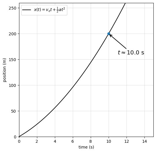
A car merges into freeway traffic on a straight, \(200\ {\rm m}\)-long on-ramp. If its initial velocity is \(v_o = 10.0\ {\rm m/s}\) and it accelerates uniformly at \(a = 2.00\ {\rm m/s^2}\), how long does it take the car to travel \(200\ {\rm m}\) up the ramp?
Fig. 3.8 Sketch of a car accelerating on a freeway ramp. Figure Credit: OpenStax: Motion with Constant Acceleration.#
The Model
The car moves in one dimension with constant acceleration along the ramp. We choose the start of the ramp as the origin and take the direction of motion as positive. The known displacement, initial velocity, and acceleration determine the travel time through the constant-acceleration position equation.
The Math
For constant acceleration, the position is given by
With the start of the ramp as the origin, \(x_o=0\) and \(x=200\ {\rm m}\), so the position equation gives
Applying the quadratic formula to the equation \(t^2+10.0t-200=0\) gives
The two mathematical roots are \(t=10.0\ {\rm s}\) and \(t=-20.0\ {\rm s}\). The negative root corresponds to a time before the modeled motion begins, so the physical travel time is
The Conclusion
The car takes \(\boxed{10.0\ {\rm s}}\) to travel the \(200\ {\rm m}\) on-ramp. The negative mathematical root is rejected because it does not describe the time after the car begins the modeled motion.
The Verification
The Python cell below computes the position as a function of time using the same constant-acceleration equation. The numerical result confirms that the car reaches \(200\ {\rm m}\) at approximately \(10.0\ {\rm s}\).
# Verification of time for an accelerating car on a freeway ramp
import numpy as np
import matplotlib.pyplot as plt
# Given values
v0 = 10.0 # initial velocity (m/s)
a = 2.00 # acceleration (m/s^2)
x_target = 200.0 # displacement (m)
# Time array
dt = 0.01
t = np.arange(0, 15 + dt, dt)
# Position as a function of time
x = v0 * t + 0.5 * a * t**2
# Find the time when x is closest to 200 m
idx = np.argmin(np.abs(x - x_target))
t_solution = t[idx]
x_solution = x[idx]
# Print numerical result
print(f"The car reaches {x_target:.0f} m after approximately {t_solution:.2f} s.")
print(f"At that time, the computed position is {x_solution:.1f} m.")
# Plot position vs time
fig, ax = plt.subplots(figsize=(6,6),dpi=100)
ax.plot(t, x, 'k-', lw=1.5,label=r"$x(t) = v_o t + \frac{1}{2} a t^2$")
ax.scatter(t_solution, x_solution, zorder=3)
# Annotate solution point
ax.annotate(
r"$t \approx 10.0\ \mathrm{s}$",xy=(t_solution, x_solution),
xytext=(t_solution + 1.0, x_solution - 40), arrowprops=dict(arrowstyle="->",lw=1.5),fontsize=14)
ax.set_xlabel("time (s)")
ax.set_ylabel("position (m)")
ax.set_xlim(0, 15)
ax.set_ylim(0, 260)
ax.grid(True, alpha=0.4)
ax.legend(loc="upper left")
plt.show()
The car reaches 200 m after approximately 10.00 s.
At that time, the computed position is 200.0 m.
3.4.6.2. Example Problem: Acceleration of a Spaceship#
Exercise 3.10
The Problem
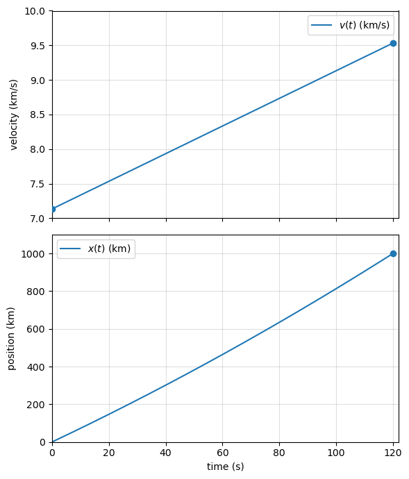
A spaceship has left Earth’s orbit and is on its way to the Moon. It accelerates at \(20.0\ {\rm m/s^2}\) for \(2\ {\rm min}\) and covers a distance of \(1000\ {\rm km}\). What are the initial and final velocities of the spaceship?
The Model
The spaceship moves in one dimension with constant acceleration. Both the initial and final velocities are unknown, so the displacement relation is used first to determine the initial velocity. The velocity-time relation is then used to determine the final velocity.
The Math
For constant acceleration, the displacement is related to initial velocity, acceleration, and time by
It is convenient to work in kilometers for position and seconds for time. Converting the acceleration and elapsed time gives
Solving the displacement equation for the initial velocity gives
The final velocity is found from the velocity-time relation, which gives
The Conclusion
The spaceship’s initial velocity is \(\boxed{7.13\ {\rm km/s}}\), and its final velocity is \(\boxed{9.53\ {\rm km/s}}\). The final velocity is larger because the spaceship accelerates in the direction of motion throughout the interval.
The Verification
The Python cell below computes the initial velocity from the displacement equation and then computes the final velocity from the velocity-time relation. The position and velocity plots confirm that the spaceship reaches \(1000\ {\rm km}\) at \(120\ {\rm s}\) while its velocity increases linearly.
# Verification of spaceship acceleration problem
import numpy as np
import matplotlib.pyplot as plt
# Given values
a = 0.02 # km/s^2
t_final = 120.0 # s
x_final = 1.0e3 # km
# Time array
dt = 0.1
t = np.arange(0, t_final + dt, dt)
# Solve for initial velocity from displacement equation
v0 = (x_final - 0.5 * a * t_final**2) / t_final
# Velocity and position as functions of time
v = v0 + a * t
x = v0 * t + 0.5 * a * t**2
# Print results
print(f"The required initial velocity is {v0:.1f} km/s.")
print(f"The final velocity after {t_final:.0f} s is {v[-1]:.1f} km/s.")
print(f"The final position after {t_final:.0f} s is {x[-1]:.1f} km.")
# Create plots
fig, axes = plt.subplots(2, 1, figsize=(6, 7), sharex=True)
# Velocity plot
axes[0].plot(t, v,label='$v(t)$ (km/s)')
axes[0].scatter([0, t_final], [v0, v[-1]], zorder=3)
axes[0].set_ylabel("velocity (km/s)")
axes[0].legend()
axes[0].grid(True, alpha=0.4)
axes[0].set_ylim(7,10)
axes[0].set_xlim(0,122)
# Position plot
axes[1].plot(t, x, label='$x(t)$ (km)')
axes[1].scatter(t_final, x[-1], zorder=3)
axes[1].set_xlabel("time (s)")
axes[1].set_ylabel("position (km)")
axes[1].legend()
axes[1].grid(True, alpha=0.4)
axes[1].set_ylim(0,1100)
axes[1].set_xlim(0,122)
plt.tight_layout()
plt.show()
The required initial velocity is 7.1 km/s.
The final velocity after 120 s is 9.5 km/s.
The final position after 120 s is 1000.0 km.
3.4.7. Two-Body Pursuit Problems#
In a two-body pursuit problem, the motions of the objects are coupled (i.e., the unknown depends on the motion of both objects). To solve these problems we write the equations of motion for each object and then solve them simultaneously to find the unknown.
Fig. 3.9 A two-body pursuit scenario where car 2 has a constant velocity and car 1 is behind with a constant acceleration. Car 1 catches up with car 2 at a later time. Figure Credit: OpenStax: Motion with Constant Acceleration.#
Checkpoint
In a pursuit problem, what condition tells us that the two objects meet?
Should their positions, velocities, or accelerations be equal?
The time and distance required for car 1 to catch car 2 (see Fig. 3.9) depends on the initial distance car 1 is from car 2 as well as the velocities of both cars and the acceleration of car 1.
The initial distance defines how far car 1 needs to travel to catch up.
The velocities of both cars and the acceleration of car 1 define the relative motion of the cars. If
\[\begin{align*} \begin{cases} \text{car 1 never catches car 2}; \quad &a_1\leq 0\ \&\ v_1 < v_2, \\ \text{car 1 keeps pace with car 2}; \quad &a_1 = 0\ \&\ v_1 = v_2, \\ \text{car 1 catches car 2}; \quad &a_1>0\ \&\ v_1 > v_2. \end{cases} \end{align*}\]
The two objects meet when their positions are equal at the same time:
Their velocities do not need to be equal when they meet. In fact, in many pursuit problems the catching object has a different velocity at the instant it reaches the other object.
For the common case where car 2 moves with constant velocity and car 1 starts behind it, car 1 catches car 2 if the position equation has a physically meaningful positive-time solution. If no positive-time solution exists, then car 1 does not catch car 2 within the modeled motion.
3.4.7.1. Example Problem: Cheetah Catching a Gazelle#
Exercise 3.11
The Problem
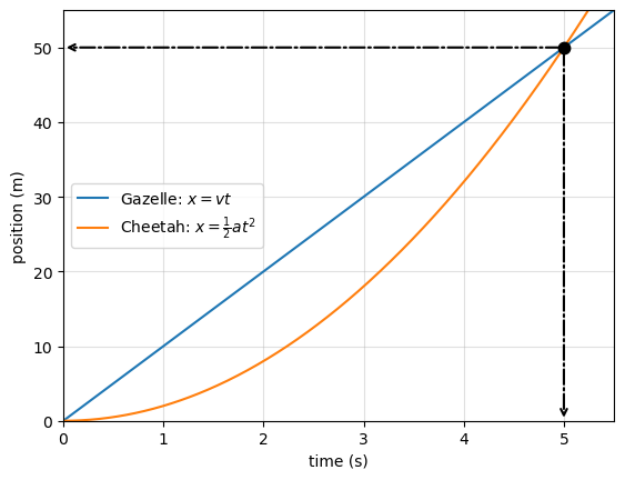
A cheetah waits in hiding behind a bush. The cheetah spots a gazelle running past at \(10\ {\rm m/s}\). At the instant the gazelle passes the cheetah, the cheetah accelerates from rest at \(4.0\ {\rm m/s^2}\) to catch the gazelle.
a. How long does it take for the cheetah to catch the gazelle?
b. What is the displacement of the gazelle and the cheetah?
The Model
This is a one-dimensional pursuit problem involving two objects. We choose the point where the gazelle passes the cheetah as the origin and take the direction of motion as positive. The gazelle moves with constant velocity, while the cheetah starts from rest and accelerates uniformly. The cheetah catches the gazelle when both animals have the same position at the same time.
The Math
The gazelle moves with constant velocity, so its position is
The cheetah starts from rest with constant acceleration, so its position is
(a) At the catch time, the two positions are equal, which gives
The nonzero catch time is found by dividing both sides by \(t\) and solving for \(t\), which gives
(b) The catch displacement is found by evaluating the gazelle’s position at \(t=5.0\ {\rm s}\), which gives
The cheetah’s position gives the same displacement at the catch time, which is
The Conclusion
The cheetah catches the gazelle after \(\boxed{5.0\ {\rm s}}\). Both animals have traveled \(\boxed{50\ {\rm m}}\) from the starting point when the catch occurs.
The Verification
The Python cell below computes the positions of the cheetah and gazelle as functions of time and identifies the nonzero intersection of the two curves. The numerical intersection confirms the analytical catch time and displacement.
import numpy as np
import matplotlib.pyplot as plt
# Given parameters
v_G = 10.0 # speed of gazelle in m/s
a_C = 4.0 # acceleration of cheetah in m/s^2
# Time array
dt = 0.01
t = np.arange(0, 6 + dt, dt)
# Positions
x_G = v_G * t
x_C = 0.5 * a_C * t**2
# Find catch time (minimum separation)
idx = np.where(np.abs(x_G- x_C)<1e-4)[0]
t_catch = t[idx][1] # need [1] to exclude starting time
x_catch = x_G[idx][1] # need [1] to exclude starting separation
print(f"The cheetah catches the gazelle after {t_catch:.2f} s.")
print(f"The displacement at the catch point is {x_catch:.1f} m.")
# Plot
fig, ax = plt.subplots()
ax.plot(t, x_G, label="Gazelle: $x=vt$")
ax.plot(t, x_C, label="Cheetah: $x=\\frac{1}{2}at^2$")
ax.plot(t_catch, x_catch, 'k.',ms=15,zorder=3)
# Arrows from endpoint to axes
ax.annotate("", xy=(t_catch, 0), xytext=(t_catch, x_catch),
arrowprops=dict(arrowstyle="->", lw=1.5,ls='-.'))
ax.annotate("", xy=(0, x_catch), xytext=(t_catch, x_catch),
arrowprops=dict(arrowstyle="->", lw=1.5,ls='-.'))
ax.set_xlabel("time (s)")
ax.set_ylabel("position (m)")
ax.legend(loc='center left')
ax.grid(alpha=0.4)
ax.set_xlim(0,5.5)
ax.set_ylim(0,55)
plt.show()
The cheetah catches the gazelle after 5.00 s.
The displacement at the catch point is 50.0 m.
Show code cell source
import numpy as np
import matplotlib.pyplot as plt
from matplotlib.animation import FuncAnimation
from IPython.display import HTML
# ----------------------------
# Given parameters
# ----------------------------
v_G = 10.0 # speed of gazelle in m/s
a_C = 4.0 # acceleration of cheetah in m/s^2
# Time array (use arange, not linspace)
dt = 0.01
t = np.arange(0, 5.01 + dt, dt)
# Positions
x_G = v_G * t
x_C = 0.5 * a_C * t**2
# Catch time (exclude the starting time)
idx = np.where(np.abs(x_G - x_C) < 1e-4)[0]
t_catch = t[idx][1] # [1] excludes the trivial t=0 intersection
x_catch = x_G[idx][1]
print(f"The cheetah catches the gazelle after {t_catch:.2f} s.")
print(f"The displacement at the catch point is {x_catch:.1f} m.")
# Find the animation frame closest to t_catch
i_catch = int(np.argmin(np.abs(t - t_catch)))
# ----------------------------
# Animation setup
# ----------------------------
fig, ax = plt.subplots(figsize=(9, 2.6))
xmax = max(x_G[-1], x_C[-1])
ax.set_xlim(-0.03 * xmax, 1.03 * xmax)
ax.set_ylim(-1.0, 1.0)
ax.set_yticks([])
ax.set_xlabel("position x (m)")
ax.grid(alpha=0.35)
# "Track" line
ax.hlines(0, 0, xmax, alpha=0.2)
# Dots (gazelle blue, cheetah orange)
dot_G, = ax.plot([], [], "o", ms=10, label="Gazelle")
dot_C, = ax.plot([], [], "o", ms=10, label="Cheetah")
# Catch highlight: ring + label + guide arrows
ring, = ax.plot([], [], "o", ms=18, mfc="none", mec="k", mew=2, zorder=4)
txt = ax.text(0, 0.55, "", ha="center", va="bottom")
# Two arrows from catch point to axes (hidden until catch)
# We'll draw them as line segments with arrowheads.
arr_to_x = ax.annotate("",xy=(0, 0), xytext=(0, 0),
arrowprops=dict(arrowstyle="->", lw=1.5, ls="-."))
arr_to_t = ax.annotate("",xy=(0, 0),xytext=(0, 0),
arrowprops=dict(arrowstyle="->", lw=1.5, ls="-."))
arr_to_x.set_visible(False)
arr_to_t.set_visible(False)
ax.legend(loc="upper left")
# small vertical offset so they don't overlap visually
y_G, y_C = 0.25, -0.25
def init():
dot_G.set_data([], [])
dot_C.set_data([], [])
dot_G.set_color("tab:blue")
dot_C.set_color("tab:orange")
ring.set_data([], [])
txt.set_text("")
arr_to_x.set_visible(False)
arr_to_t.set_visible(False)
return dot_G, dot_C, ring, txt, arr_to_x, arr_to_t
def update(i):
# Move dots
dot_G.set_data([x_G[i]], [y_G])
dot_C.set_data([x_C[i]], [y_C])
# Default state
ring.set_data([], [])
txt.set_text("")
arr_to_x.set_visible(False)
arr_to_t.set_visible(False)
dot_G.set_markersize(10)
dot_C.set_markersize(10)
# Highlight catch frame
if i == i_catch:
dot_G.set_markersize(14)
dot_C.set_markersize(14)
ring.set_data([x_catch], [0.0])
txt.set_position((x_catch, 0.55))
txt.set_text(f"CATCH!\n$t={t_catch:.2f}\\,\\mathrm{{s}}$ $x={x_catch:.1f}\\,\\mathrm{{m}}$")
# Arrows from catch point to axes
arr_to_x.xy = (x_catch, 0.0) # arrow head on x-axis
arr_to_x.xyann = (x_catch, 0.35) # start above
arr_to_x.set_visible(True)
arr_to_t.xy = (0.0, 0.0) # arrow head at origin
arr_to_t.xyann = (x_catch, 0.0) # start at catch point on axis line
arr_to_t.set_visible(True)
return dot_G, dot_C, ring, txt, arr_to_x, arr_to_t
anim = FuncAnimation(fig,update,frames=len(t),init_func=init,interval=40,blit=True)
plt.close(fig)
HTML(anim.to_jshtml())
The cheetah catches the gazelle after 5.00 s.
The displacement at the catch point is 50.0 m.
3.5. Free Fall#
This narration is AI-generated from the course text.
3.5.1. Gravity#
Until Galileo Galilei showed otherwise, people believed that a heavier object has a greater acceleration in a free fall. We know now that this is not the case.
In the absence of air resistance, heavy objects arrive at the ground at the same time as lighter objects when dropped from the same height.
In the real world, air resistance can cause a lighter object to fall slower than a heavier object of the same size. A tennis ball reaches the ground after a baseball dropped at the same time, although the difference is not large. Air resistance opposes the motion of an object through the air and friction between objects also opposes motion between them.
Free fall is when an object falls without air resistance or friction. The force of gravity causes objects to fall toward the center of the Earth, where this acceleration is also called the acceleration due to gravity.
Near Earth’s surface (or for small changes in altitude) the acceleration due to gravity is constant, which means we can apply the kinematic equations to any falling object (where air resistance and friction are negligible), including spherical cows.
Acceleration due to gravity is given its own symbol \(g\), where it is nearly constant at any location on Earth’s surface with the average value
The value of \(g\) can vary from \(9.78 - 9.83\ {\rm m/s^2}\) depending on latitude, altitude, underlying geological formations, and local topography. Here we use \(g = 9.81\ {\rm m/s^2}\) unless otherwise specified.
Checkpoint
A ball is thrown straight upward. At the highest point, its velocity is momentarily zero.
What is its acceleration at that instant?
The direction of acceleration due to gravity \(g\) is defined to be downward (i.e., toward Earth’s center). Its direction defines what we call vertical.
Note
The acceleration \(a\) in the kinematic equations has the value \(+g\) or \(-g\) depending on how we define our coordinate system. If we define the
upward direction as positive, then \(a=-g=-9.81\ {\rm m/s^2}\).
downward direction as positive, then \(a=g=9.81\ {\rm m/s^2}\).
3.5.2. One-Dimensional Motion Involving Gravity#
Consider vertical (up-and-down) motion with no air resistance or friction, where these assumptions mean the velocity is also vertical. There are some statements about the initial velocity of an object as it enters or leaves free fall. The object is in free fall after it has left contact with whatever held or threw it.
If an object is dropped, we know the initial velocity is zero when in free fall (i.e., \(v_o = 0\)).
If the object is thrown, it has the same speed in free fall as it did before it was released (i.e., \(v_o\) is defined at release).
When in free fall, the motion is 1D and has constant acceleration of magnitude \(g\). When the object comes in contact with the ground (or any other object), it is no longer in free fall (i.e., \(a \neq g\)).
We represent the vertical displacement with the symbol \(y\) and write the following kinematic equations for objects in free fall. We assume that the positive direction is upward, which gives
When solving free fall problems, its helpful to follow this strategy:
Decide on the sign of \(g\) (i.e., is positive upward or downward). In some problems, it may be useful to have \(+g\) indicating the positive direction is downward.
DRAW A SKETCH of the problem. Visualizing the problem can be a useful first step. Don’t worry about artistic quality.
Identify the knowns and unknowns from the problem description.
Match the kinematic equations with the knowns and unknowns.
3.5.2.1. Example Problem: Free Fall of a Ball#
Exercise 3.12
The Problem
Fig. 3.10 shows the positions of a ball, at \(1\ {\rm s}\) intervals, with an initial velocity of \(4.9\ {\rm m/s}\) downward, that is thrown from the top of a \(98\ {\rm m}\)-high building. (a) How much time elapses before the ball reaches the ground? (b) What is the velocity when it arrives at the ground?
Fig. 3.10 The positions and velocities at \(1\ {\rm s}\) intervals of a ball thrown downward from a tall building at \(4.9\ {\rm m/s}\). Figure Credit: OpenStax: Free-fall.#
The Model
The ball moves vertically in one dimension under constant gravitational acceleration. We choose the top of the building as the origin, upward as positive, and downward as negative. With this sign convention, both the initial velocity and acceleration are negative.
The Math
(a) For constant acceleration, the vertical position is given by
The ball starts at the origin, the ground is at \(y=-98\ {\rm m}\), the initial velocity is downward, and \(a=-g\) with \(g=9.81\ {\rm m/s^2}\), so the impact condition gives
Solving this quadratic equation gives the mathematical roots \(t=-5.0\ {\rm s}\) and \(t=4.0\ {\rm s}\). The negative root is not physical for the motion after release, so the elapsed time is
(b) The velocity at the ground is found from the velocity-time equation, which gives
The Conclusion
The ball reaches the ground after \(\boxed{4.0\ {\rm s}}\). Its velocity just before impact is \(\boxed{-44\ {\rm m/s}}\), meaning the ball is moving downward at \(44\ {\rm m/s}\).
The Verification
The Python cell below computes the ball’s position and velocity as functions of time using the same constant-acceleration equations. The numerical values at the impact time confirm the analytical time and downward impact velocity.
import numpy as np
import matplotlib.pyplot as plt
# Given values
y0 = 0.0 # initial position (m)
v0 = -4.9 # initial velocity (m/s)
a = -9.81 # acceleration (m/s^2)
# Time array
dt = 0.01
t = np.arange(0, 6 + dt, dt)
# Position and velocity
y = y0 + v0*t + 0.5*a*t**2
v = v0 + a*t
# Find impact time (closest point to y = -98 m)
idx = np.argmin(np.abs(y + 98))
t_hit = t[idx]
v_hit = v[idx]
print(f"The ball reaches the ground after approximately {t_hit:.2f} s.")
print(f"The velocity of the ball at the ground is {v_hit:.1f} m/s.")
# Plot
fig, ax = plt.subplots(2, 1, figsize=(6, 6), sharex=True)
ax[0].plot(t, y)
ax[0].scatter(t_hit, y[idx], zorder=3)
ax[0].set_ylabel("position (m)")
ax[0].grid(alpha=0.4)
ax[0].set_ylim(-100,2)
ax[0].set_xlim(0,4)
ax[0].minorticks_on()
ax[1].plot(t, v)
ax[1].scatter(t_hit, v_hit, zorder=3)
ax[1].set_xlabel("time (s)")
ax[1].set_ylabel("velocity (m/s)")
ax[1].grid(alpha=0.4)
ax[1].set_ylim(-45,-0)
ax[1].set_xlim(0,4)
ax[1].minorticks_on()
plt.show()
The ball reaches the ground after approximately 4.00 s.
The velocity of the ball at the ground is -44.1 m/s.
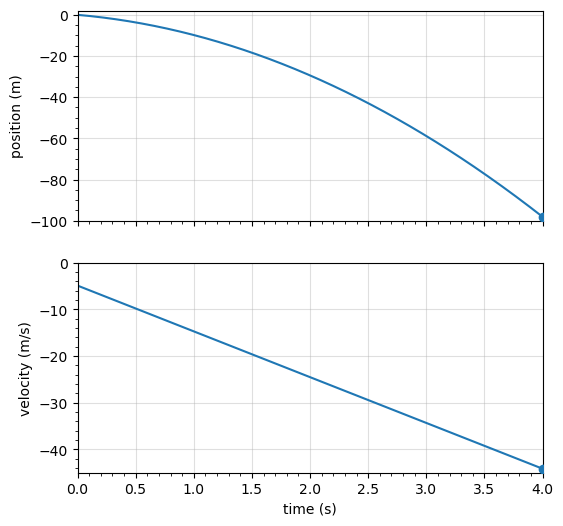
3.5.2.2. Example Problem: Rocket Booster Motion#
Exercise 3.13
The Problem
A small rocket blasts off and travels straight upward. When at a height of \(5.0\ {\rm km}\) and velocity of \(200.0\ {\rm m/s}\), it releases its booster. (a) What is the maximum height the booster attains? What is the velocity of the booster at a height of \(6.0\ {\rm km}\)? Neglect air resistance.
The Model
After release, the booster moves vertically under constant gravitational acceleration, with air resistance neglected. We choose upward as the positive direction and place the origin at the release point. The booster’s acceleration is downward, so it is negative in this coordinate system.
The Math
For constant acceleration, velocity and displacement are related by
Since the acceleration is gravitational and downward, \(a=-g\), so this relation becomes
(a) At the maximum height, the booster momentarily has zero velocity, so the velocity-displacement relation gives
Solving for the additional height above the release point gives
Using \(g=9.81\ {\rm m/s^2}\), the additional height above the release point is
The maximum height above Earth’s surface is the release height plus the additional height, which gives
(b) A height of \(6.0\ {\rm km}\) above Earth’s surface is \(1.0\ {\rm km}\) above the release point, which is
The speed at this height is found from the same velocity-displacement equation, which gives
Taking the square root gives two possible velocity directions at this height, so the velocity is
The Conclusion
The booster reaches a maximum height of \(\boxed{7.0\ {\rm km}}\) above Earth’s surface. At a height of \(6.0\ {\rm km}\), its velocity can be \(\boxed{+140\ {\rm m/s}}\) while moving upward or \(\boxed{-140\ {\rm m/s}}\) while moving downward.
The Verification
The Python cell below models the booster’s height and velocity after release using constant downward acceleration. The numerical peak height and the two velocity values at \(1.0\times10^3\ {\rm m}\) above the release point confirm the analytical results.
import numpy as np
import matplotlib.pyplot as plt
from matplotlib.collections import LineCollection
# Given parameters (after release)
g = 9.81 # m/s^2
v0 = 200.0 # m/s
y0 = 0.0 # m (release point as origin)
y_target = 1000.0 # m (this corresponds to 6.0 km altitude)
# Time array (use arange, not linspace)
dt = 0.001
t_max = 2 * v0 / g # time to go up and come back to y=0
t = np.arange(0.0, t_max + dt, dt)
# Kinematics
y = y0 + v0 * t - 0.5 * g * t**2
v = v0 - g * t
# (a) Max height (relative + absolute)
idx_peak = np.argmin(np.abs(v)) # closest to v=0
y_peak = y[idx_peak] # relative max height (m)
alt_peak_km = 5.0 + y_peak / 1000.0 # add 5.0 km release altitude
print(f"The maximum height above the release point is {y_peak:.0f} m.")
print(f"The maximum altitude above Earth's surface is {alt_peak_km:.1f} km.")
# (b) Two velocity solutions at y = 1000 m
# Find times where y crosses y_target (within tolerance) and keep the first crossing in each branch.
tol = 0.5 # meters (tolerance for selecting near-target points)
idx = np.where(np.abs(y - y_target) < tol)[0]
# Split into rising vs falling using sign of v (positive = rising, negative = falling)
idx_up = idx[v[idx] > 0]
idx_dn = idx[v[idx] < 0]
# Pick representative indices (first from each list)
i_up = idx_up[0]
i_dn = idx_dn[0]
t_up, v_up = t[i_up], v[i_up]
t_dn, v_dn = t[i_dn], v[i_dn]
print(f"At y = {y_target:.0f} m on the way up, the time is {t_up:.1f} s and the velocity is {v_up:.0f} m/s.")
print(f"At y = {y_target:.0f} m on the way down, the time is {t_dn:.1f} s and the velocity is {v_dn:.0f} m/s.")
# Plot v vs y, showing BOTH solutions at y_target
fig, ax = plt.subplots(figsize=(6,6),dpi=120)
#ax.plot(y, v, label="Booster trajectory: $v(y)$")
# Create line segments for (y, v)
points = np.array([y, v]).T.reshape(-1, 1, 2)
segments = np.concatenate([points[:-1], points[1:]], axis=1)
# LineCollection colored by time
lc = LineCollection(segments, cmap="viridis",label="Booster trajectory: $v(y)$")
lc.set_array(t) # color mapped to time
lc.set_linewidth(2)
line = ax.add_collection(lc)
ax.axvline(y_target, linestyle="--", linewidth=1.5, color = 'k',label=r"Target: $y=1000\ \mathrm{m}$")
# Mark the two solutions
ax.plot(y_target, v_up, "ko", zorder=3)
ax.plot(y_target, v_dn, "ko", zorder=3)
cbar = plt.colorbar(line, ax=ax)
cbar.set_label("time (s)")
# Annotations
ax.annotate(rf"$v=+{v_up:2.0f}\ \mathrm{{m/s}}$",xy=(y_target, v_up), xytext=(y_target + 150, v_up + 15),
arrowprops=dict(arrowstyle="->", lw=1.5, ls='-.'))
ax.annotate(rf"$v={v_dn:2.0f}\ \mathrm{{m/s}}$",xy=(y_target, v_dn), xytext=(y_target + 150, v_dn - 25),
arrowprops=dict(arrowstyle="->", lw=1.5, ls='-.'))
ax.set_xlabel("height relative to release, $y$ (m)")
ax.set_ylabel("velocity, $v$ (m/s)")
ax.grid(alpha=0.4)
ax.set_xlim(0, np.max(y) * 1.05)
ax.set_ylim(np.min(v) * 1.05, np.max(v) * 1.05)
ax.legend(loc="center left")
plt.show()
The maximum height above the release point is 2039 m.
The maximum altitude above Earth's surface is 7.0 km.
At y = 1000 m on the way up, the time is 5.8 s and the velocity is 143 m/s.
At y = 1000 m on the way down, the time is 34.9 s and the velocity is -143 m/s.
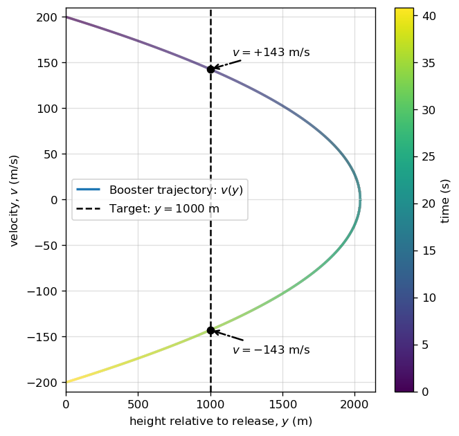
3.6. Finding Velocity and Displacement from Acceleration#
This narration is AI-generated from the course text.
3.6.1. Kinematic Equations from Integral Calculus#
In later chapters, we’ll start with a force that depends on the acceleration \(a\). There is some insight into why calculus is useful to determine (or remember) the kinematic equations.
Let’s begin with a particle with an acceleration \(a(t)\), which we can express as in differential form by
in terms of the the velocity function. One way to solve a differential equation is to take the indefinite integral of both sides, where we get
and \(C_1\) represents a constant of integration.
Note
The integral of the derivative of a function is simply the function. For example,
The integral is also called the anti-derivative because it is like an inverse operation of the derivative. This is similar to how \(\sqrt{x^2} = x\), if we take only the positive root.
Using the antiderivative property from calculus, we have
We can employ the same procedure to write the velocity function in terms of the position function, as
and with the integral, we have
where \(C_2\) is a second constant of integration.
Checkpoint
If acceleration is the slope of the velocity graph, what does the area under an acceleration-versus-time graph represent?
Using these integrals, we can derive the kinematic equations. Since \(a(t)\) can be any function, let’s assume that \(a(t)=at^0=a=\text{constant}\). Then we can evaluate the velocity function as
where \(C_1 = v_o = v(0)\). Then we can substitute into the integral to get the position function, or
where \(C_2 =x_o=x(0)\).
3.6.1.1. Example Problem: Motion of a Motorboat#
Exercise 3.14
The Problem
A motorboat is traveling at a constant velocity of \(5.0\ {\rm m/s}\) when it begins to accelerate opposite the direction of motion to arrive at a dock. Its acceleration is \(a(t) = -\frac{1}{4}t\ {\rm m/s^3}\). (a) What is the velocity function of the motorboat? (b) At what time does the velocity reach zero? (c) What is the position function of the motorboat? (d) What is the displacement of the motorboat from the time it begins to decelerate to the time its velocity reaches zero? (e) Graph the velocity and position functions.
The Model
The motorboat moves in one dimension along the direction of its initial motion. The acceleration is time dependent and points opposite the motion, so velocity is found by integrating acceleration, and position is found by integrating velocity. We choose the initial position as the origin and measure time from the instant the deceleration begins.
The Math
(a) Velocity is found by integrating the acceleration function with respect to time, which gives
The integration constant is determined by the initial velocity \(v(0)=5.0\ {\rm m/s}\), which gives \(C_1=5.0\ {\rm m/s}\). The velocity function is therefore
(b) The stopping time occurs when the velocity reaches zero, so the velocity function gives
Solving this equation for the positive time gives
(c) Position is found by integrating the velocity function with respect to time, which gives
The initial position is chosen to be \(x(0)=0\), so \(C_2=0\). The position function is therefore
(d) The displacement while the boat slows to rest is found by evaluating the position function at \(t=6.3\ {\rm s}\), which gives
(e) The velocity and position graphs are generated from the functions derived above. The velocity graph decreases to zero at \(t=6.3\ {\rm s}\), and the position graph reaches its maximum value at that same time.
The Conclusion
The motorboat’s velocity function is \(\boxed{v(t)=\left(5.0-\frac{1}{8}t^2\right){\rm m/s}}\), and its position function is \(\boxed{x(t)=\left(5.0t-\frac{1}{24}t^3\right){\rm m}}\). The velocity reaches zero at \(\boxed{6.3\ {\rm s}}\), after the boat has traveled \(\boxed{21\ {\rm m}}\). The velocity graph crosses zero at the same time that the position graph reaches its maximum.
The Verification
The Python cell below evaluates the derived velocity and position functions over time. The plots confirm that the velocity reaches zero at about \(6.3\ {\rm s}\) and that the position is about \(21\ {\rm m}\) at that instant.
import numpy as np
import matplotlib.pyplot as plt
# Time array
dt = 0.01
t = np.arange(0, 10 + dt, dt)
# Functions
v = 5.0 - (1/8)*t**2
x = 5.0*t - (1/24)*t**3
# Find stopping time
idx = np.where(np.abs(v) < 1e-2)[0][0]
t_stop = t[idx]
x_stop = x[idx]
print(f"The motorboat's velocity reaches zero after {t_stop:.2f} s.")
print(f"The displacement of the motorboat when it stops is {x_stop:.2f} m.")
# Plot setup
fig, ax = plt.subplots(2, 1, figsize=(5, 8), dpi=100)
data = [dict(f=v, flabel="velocity (m/s)", label=r"$v(t)=5-\frac{1}{8}t^2$",ylim=(-8, 5), marker_y=0),
dict(f=x, flabel="position (m)", label=r"$x(t)=5t-\frac{1}{24}t^3$",ylim=(0, 23), marker_y=x_stop)]
for i, cfg in enumerate(data):
ax[i].plot(t, cfg["f"], "k-", lw=1.5, label=cfg["label"])
ax[i].scatter(t_stop, cfg["marker_y"], zorder=3)
ax[i].set(xlabel="time (s)",ylabel=cfg["flabel"],xlim=(0, 10),ylim=cfg["ylim"])
ax[i].grid(alpha=0.4)
ax[i].legend()
# --- Annotations specific to each panel ---
# Velocity panel arrows
ax[0].annotate("", xy=(0, 0), xytext=(t_stop, 0),
arrowprops=dict(arrowstyle="->", lw=1.5, ls='-.'))
ax[0].annotate("", xy=(t_stop, -8), xytext=(t_stop, 0),
arrowprops=dict(arrowstyle="->", lw=1.5, ls='-.'))
# Position panel reference line + arrow
ax[1].axhline(x_stop, linestyle='--', alpha=0.5, color="r")
ax[1].annotate("", xy=(t_stop, x_stop), xytext=(t_stop, 0),
arrowprops=dict(arrowstyle="->", lw=1.5, ls='-.'))
plt.tight_layout()
plt.show()
The motorboat's velocity reaches zero after 6.32 s.
The displacement of the motorboat when it stops is 21.08 m.
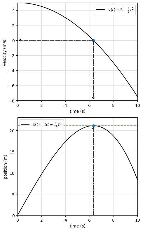
3.7. Supplemental Review#
These videos provide a fast review of ideas used in this chapter:
Crash Course Physics #1: Motion in a Straight Line — position, velocity, acceleration, and one-dimensional motion.
Crash Course Physics #2: Derivatives — the calculus connection between position, velocity, and acceleration.
Crash Course Physics #3: Integrals — the calculus connection between acceleration, velocity, and position.
Use these videos after you have worked through the chapter. They are best for reinforcing the big picture, not for learning the problem-solving method for the first time.
3.8. In-class Problems#
Problem 1
A cyclist rides \(8.0\) km east for \(20\) minutes, then turns and heads west for \(8\) minutes, covering \(3.2\) km. Finally, the cyclist rides east for \(16\) km, which takes \(40\) minutes.
(a) What is the final displacement of the cyclist?
(b) What is the cyclist’s average velocity over the entire trip?
Problem 2
An object has a position function \(x(t) = 5t\ {\rm m}.\)
(a) What is the velocity as a function of time?
(b) Graph the position function and the velocity function.
Problem 3
Assume an intercontinental ballistic missile goes from rest to a suborbital speed of \(6.5\ {\rm km/s}\) in \(60\ {\rm s}\) (the actual speed and time are classified).
(a) What is its average acceleration in \({\rm m/s^2}\)?
(b) What is its average acceleration in multiples of \(g = 9.81\ {\rm m/s^2}\)?
Problem 4
An express train passes through a station. It enters with an initial velocity of \(22\ {\rm m/s}\) and accelerates opposite the direction of motion at a rate of \(0.15\ {\rm m/s^2}\) as it goes through. The station is \(210\ {\rm m}\) long.
(a) How fast is the train when the nose leaves the station?
(b) How long is the nose of the train in the station?
(c) If the train is \(130\ {\rm m}\) long, what is the velocity of the end of the train as it leaves the station?
(d) When does the end of the train leave the station?
Problem 5
A diver bounces straight up from a diving board, avoids the board on the way down, and falls feet first into a pool. She starts with a velocity of \(4.00\ {\rm m/s}\), and her takeoff point is \(1.80\ {\rm m}\) above the pool.
(a) What is her highest point above the board?
(b) How long are her feet in the air?
(c) What is her velocity when her feet hit the water?
3.9. Homework#
3.9.1. Conceptual Problems#
Problem 1
During a given time interval the average velocity of an object is zero. What can you conclude about its displacement over the time interval?
Problem 2
An object that is thrown straight up falls back to Earth. This is one-dimensional motion.
(a) When is its velocity zero?
(b) Does its velocity change direction?
(c) Does the acceleration have the same sign on the way up as on the way down?
3.9.2. Problems#
Problem 3
A particle moves along the \(x\)-axis according to \(x(t) = 10t - 2t^2\ {\rm m}\).
(a) What is the instantaneous velocity at \(t = 2\ {\rm s}\) and \(t = 3\ {\rm s}\)?
(b) What is the instantaneous speed at these times?
(c) What is the average velocity between \(t = 2\ {\rm s}\) and \(t = 3\ {\rm s}\)?
Problem 4
An airplane, starting from rest, moves down the runway at constant acceleration for \(18\ {\rm s}\) and then takes off at a speed of \(60\ {\rm m/s}\). What is the average acceleration of the plane?
Problem 5
A fireworks shell is accelerated from rest to a velocity of \(65\ {\rm m/s}\) over a distance of \(0.25\ {\rm m}\).
(a) Calculate the acceleration.
(b) How long did the acceleration last?
Problem 6
(a) Calculate the height of a cliff if it takes \(2.35\ {\rm s}\) for a rock to hit the ground when it is thrown straight up from the cliff with an initial velocity of \(8.00\ {\rm m/s}\).
(b) How long a time would it take to reach the ground if it is thrown straight down with the same speed?