8. Potential Energy and Conservation of Energy#
Jul 20, 2026 | 7873 words | 52 min read
Chapter roadmap
This chapter turns work into a more flexible bookkeeping tool by introducing potential energy and then combining potential and kinetic energy into mechanical energy. The goal is to decide when energy can be transferred back and forth within a system and when energy leaves the mechanical system through non-conservative work.
As you read, focus on three questions:
How does the choice of system determine which forms of potential energy belong in the problem?
How can the same physical motion be described using work, potential energy, or conservation of mechanical energy?
How do energy diagrams show allowed motion, turning points, and equilibrium?
These ideas let you solve motion problems without always tracking the full path or solving for the acceleration at every instant.
8.1. Potential Energy of a System#
The work done on an object by gravity (near Earth’s surface) is a function only of the displacement \(\Delta y\) (or a height \(h\)). This property allows us to define a different kind of energy for the system, which is called potential energy (in contrast to the kinetic energy).
8.1.1. Potential Energy Basics#
Consider the kicking of a football (see Fig. 8.1). Ignoring friction and air resistance, we begin the analysis immediately after the kick, or at the start of the projectile motion of the ball.
As the football rises, the work done by the gravitational force on the ball is negative, because the ball’s displacement is positive vertically and the gravitational force is negative vertically.
The ball slows down until it reaches its highest point in the motion, thereby decreasing the ball’s kinetic energy.
The loss in kinetic energy translates to a gain in the gravitational potential energy of the football-Earth system.
Fig. 8.1 As a football starts its descent toward the receiver, gravitational potential energy is converted back into kinetic energy. During the upward part of the motion, kinetic energy decreases while gravitational potential energy increases; during the downward part, the transfer reverses. Image Credit: OpenStax: Potential Energy of a System.#
As the football falls toward Earth, the work done on the football is now positive, because the displacement and the gravitational force both point in the same direction (vertically downward).
The ball speeds up, which indicates an increase in kinetic energy.
Therefore, energy is converted from gravitational potential energy back into kinetic energy.
Based on this scenario, we define the difference in potential energy from point \(A\) to \(B\) as the negative of the work done, or
We call this a potential energy difference, not just an absolute potential energy. Thus, we define the potential energy relative to a given position \(\vec{r}\) and initial position \(\vec{r}_o\). We do this by rewriting the potential energy function as
Note
The choice of the potential energy at a starting location \(\vec{r}_o\) is arbitrary and we choose the most convenient starting position depending on the problem. Even though we made an arbitrary choice, we must stick with it and the rest of the problem must be solved consistently with this assumption.
There are some natural (i.e., well-accepted) choices. For example,
the lowest height in a problem is usually defined as zero potential energy,
or if an object is in space, the farthest point away from the system is defined as zero potential energy.
Then the potential energy with respect to zero at \(\vec{r}_o\) is just
As long as there is no friction (or air resistance), the change in kinetic energy of the football equals the negative of the change in gravitational potential energy of the football. This can be generalized to
Checkpoint
If you change the zero reference level for gravitational potential energy, does the change in gravitational potential energy between two fixed heights change? Explain briefly.
8.1.1.1. Example Problem: Basic Properties of Potential Energy#
Exercise 8.1
The Problem
A particle moves along the \(x\)-axis under the action of a force given by \(F = -a x^2\), where \(a = 3\ \mathrm{N/m^2}\).
(a) What is the difference in its potential energy as it moves from \(x_A = 1\ \mathrm{m}\) to \(x_B = 2\ \mathrm{m}\)?
(b) What is the particle’s potential energy at \(x = 1\ \mathrm{m}\) with respect to a given \(0.5\ \mathrm{J}\) of potential energy at \(x = 0\)?
Show worked solution
The Model
The system consists of a single particle constrained to move along the \(x\)-axis. The force acting on the particle depends only on its position along the \(x\)-axis and points along the same axis, with the negative sign indicating that the force acts opposite the direction of increasing \(x\). No other forces act on the particle.
The motion is treated as one-dimensional, with positive displacement defined in the \(+x\) direction. Because the force depends only on position and not on the path taken, it is conservative, and the work done by the force depends only on the initial and final positions. A potential energy function can therefore be defined for this system.
The Math
For a conservative force, the change in potential energy between two points is defined as the negative of the work done by the force.
The work done by a force during an infinitesimal displacement is given by the dot product of the force and the displacement. Because both the force and the displacement lie along the \(x\)-axis, this dot product reduces to ordinary multiplication:
(a) The change in potential energy between \(x_A\) and \(x_B\) is obtained by integrating the work expression between the initial and final positions and applying the definition of potential energy difference. This is done mathematically by:
Evaluating the integral gives
where we can substitute the given values,
(b) The potential energy function is found by integrating the force with respect to position and introducing a constant of integration that reflects the chosen reference level. From the integration, we have
The value of the constant is determined using the given reference condition \(U(0) = 0.5\ \mathrm{J}\), which gives
Substituting \(x = 1\ \mathrm{m}\) into the potential energy function yields
The Conclusion
The particle’s potential energy increases by \(7\ \mathrm{J}\) as it moves from \(x = 1\ \mathrm{m}\) to \(x = 2\ \mathrm{m}\). When the potential energy is defined to be \(0.5\ \mathrm{J}\) at \(x = 0\), the potential energy at \(x = 1\ \mathrm{m}\) is \(1.5\ \mathrm{J}\). These results follow directly from the conservative, position-dependent nature of the force.
The Verification
The potential energy difference is verified by evaluating the potential energy function at \(x = 1\ \mathrm{m}\) and \(x = 2\ \mathrm{m}\) and confirming that their difference equals \(7\ \mathrm{J}\).
import numpy as np
a = 3.0 # N/m^2
def U(x):
return (1/3)*a*x**3 + 0.5
U1 = U(1.0)
U2 = U(2.0)
delta_U = U2 - U1
print("The potential energy at x = 1 m is %.1f J." % np.round(U1, 1))
print("The potential energy at x = 2 m is %.1f J." % np.round(U2, 1))
print("The change in potential energy is %.0f J." % np.round(delta_U, 0))
8.1.2. Systems of Several Particles#
A system of interest could contain several particles. The difference in potential energy of the system is the negative work done by the gravitational or elastic (i.e., conservative) forces. The potential energy depends mainly on the initial and final positions of the particles, as well as some parameters that characterize the interaction (e.g., mass for gravity or spring constant for a Hooke’s law force).
Potential energy is a property of the interactions between objects in a chosen system, and not just a property of each object.
8.1.3. Types of Potential Energy#
For each type of interaction in a system, you can label a corresponding type of potential energy. The total potential energy of the system is the sum of the potential energies of all types.
This follows from the additive property of the dot product that we found when computing the work done.
8.1.3.1. Gravitational potential energy near Earth’s surface#
Consider one (or more) particles near Earth’s surface. The gravitational force on each particle is just its weight (\(mg\)) near the surface acting vertically down.
According to Newton’s 3rd law, a particle exerts a force on Earth of equal magnitude but in the opposite direction.
Newton’s 2nd law tells us that the magnitude of acceleration is measured weight divided by the mass (i.e., \(g\)).
Since the ratio of the mass of any ordinary object to Earth’s mass is vanishingly small, the motion of Earth can be completely neglected. Therefore, we consider the particle (or a system of particles) subject to the uniform gravitational force of Earth.
The work done on a body by Earth’s uniform gravitational force (near the surface) depends on the mass of the body \(m\), the acceleration due to gravity \(g\), and the difference in height \(h\) the body traveled. By definition, this work is the negative of the difference in the gravitational potential energy or
We define the gravitational potential energy function (near Earth’s surface) as
You can choose the value of the constant, where the most convenient constant to choose is zero for when \(y=0\). This corresponds to the lowest position in the problem.
8.1.3.1.1. Example Problem: Gravitational Potential Energy of a Hiker#
Exercise 8.2
The Problem
The summit of Great Blue Hill in Milton, MA, is \(147\ \mathrm{m}\) above its base and has an elevation above sea level of \(195\ \mathrm{m}\). A \(75\ \mathrm{kg}\) hiker ascends from the base to the summit. What is the gravitational potential energy of the hiker–Earth system with respect to zero gravitational potential energy at base height, when the hiker is (a) at the base of the hill, (b) at the summit, and (c) at sea level, afterward?
Show worked solution
The Model
The system consists of the hiker and the Earth, treated together so that gravitational potential energy is an internal energy of the system. The motion is vertical, and air resistance is neglected. The gravitational field near Earth’s surface is approximated as uniform. The vertical coordinate \(y\) is defined to be positive upward, with the base of the hill chosen as the reference height where the gravitational potential energy is zero. With this choice, the constant of integration is determined by the reference condition at the base.
The Math
Gravitational potential energy in a uniform gravitational field depends on the vertical position of the system relative to the chosen reference height and is given by \(U = m g y + C\).
(a) At the base of the hill, the vertical coordinate is \(y = 0\) by definition of the reference level, so the gravitational potential energy is
(b) At the summit, the hiker is \(147\ \mathrm{m}\) above the base, so \(y = 147\ \mathrm{m}\). Substituting this value into the gravitational potential energy expression gives
(c) Sea level is \(195\ \mathrm{m}\) below the summit, which places it \(48\ \mathrm{m}\) below the base. With upward taken as positive, the vertical coordinate at sea level is therefore \(y = -48\ \mathrm{m}\). Substituting this value gives
The Conclusion
With gravitational potential energy defined to be zero at the base of the hill, the hiker–Earth system has zero gravitational potential energy at the base, \(1.08 \times 10^{5}\ \mathrm{J}\) at the summit, and \(-3.53 \times 10^{4}\ \mathrm{J}\) at sea level. The negative value at sea level reflects that this position lies below the chosen reference height, not that the energy is physically problematic.
The Verification
The results are verified by recomputing the gravitational potential energy using \(U = m g y\) at each vertical position relative to the base height and confirming that the differences in potential energy correspond to the associated height changes.
import numpy as np
m = 75.0 # kg
g = 9.81 # m/s^2
y_base = 0.0
y_summit = 147.0
y_sea = -48.0
U_base = m * g * y_base
U_summit = m * g * y_summit
U_sea = m * g * y_sea
print("The gravitational potential energy at the base is %d J." % np.round(U_base, 0))
print("The gravitational potential energy at the summit is %d J." % np.round(U_summit, 0))
print("The gravitational potential energy at sea level is %d J." % np.round(U_sea, 0))
8.1.3.2. Elastic potential energy#
The work done by a perfectly elastic spring (in 1D) depends only on the spring constant \(k\) and the squares of the displacements from the unstretched position (\(x^2-x_o^2\)). This work involves only the properties of a Hooke’s law interaction and not the properties of real springs and whatever is attached to them.
We define the difference of elastic potential energy for a spring force as the negative of the work done by the spring force. Thus,
where the object attached to the spring travels from point \(A\) to point \(B\). The potential energy function corresponding to this difference is
If the spring force is the only force, it is simplest to take the zero of potential energy at \(x=0\). This corresponds to when the spring is at its unstretched length.
Checkpoint
For a stretched spring, what physical position naturally makes the elastic potential energy equal to zero?
8.1.3.2.1. Example Problem: Spring Potential Energy#
Exercise 8.3
The Problem
A system contains a perfectly elastic spring, with an unstretched length of \(20\ \mathrm{cm}\) and a spring constant of \(4\ \mathrm{N/cm}\). (a) How much elastic potential energy does the spring contribute when its length is \(23\ \mathrm{cm}\)? (b) How much more potential energy does it contribute if its length increases to \(26\ \mathrm{cm}\)?
Show worked solution
The Model
The system consists of a single ideal spring that obeys Hooke’s law and stores elastic potential energy when stretched or compressed from its unstretched length. The spring is assumed to be perfectly elastic, with no energy losses, so its elastic potential energy depends only on the magnitude of the displacement from equilibrium. The displacement \(x\) is defined as the difference between the current length of the spring and its unstretched length, measured along the axis of the spring. The reference configuration for zero elastic potential energy is the unstretched length. Because the spring constant is given in \(\mathrm{N/cm}\), lengths and displacements are treated consistently in centimeters.
The Math
Elastic potential energy for an ideal spring is given by \(U = \tfrac{1}{2} k x^2\), where \(k\) is the spring constant and \(x\) is the displacement from the unstretched length.
(a) When the spring length is \(23\ \mathrm{cm}\), the displacement from the unstretched length is \(x = 3\ \mathrm{cm}\). Substituting this displacement into the elastic potential energy expression gives
(b) When the spring length increases to \(26\ \mathrm{cm}\), the displacement is \(x = 6\ \mathrm{cm}\). Substituting this value gives
The additional elastic potential energy contributed relative to part (a) is therefore
The Conclusion
When the spring is stretched to \(23\ \mathrm{cm}\), it stores \(0.18\ \mathrm{J}\) of elastic potential energy. Increasing the length to \(26\ \mathrm{cm}\) increases the stored energy to \(0.72\ \mathrm{J}\), which is an additional \(0.54\ \mathrm{J}\). These results follow directly from the quadratic dependence of elastic potential energy on displacement and from maintaining a consistent unit system throughout the calculation.
The Verification
The results are verified by computing the elastic potential energy using \(U = \tfrac{1}{2} k x^2\) with the displacement expressed in centimeters and confirming the difference between the two energies.
import numpy as np
k = 4.0 # N/cm
x1 = 3.0 # cm
x2 = 6.0 # cm
U1 = 0.5 * k * x1**2
U2 = 0.5 * k * x2**2
dU = U2 - U1
print("The elastic potential energy at 23 cm is %.2f J." % np.round(U1, 2))
print("The elastic potential energy at 26 cm is %.2f J." % np.round(U2, 2))
print("The additional potential energy is %.2f J." % np.round(dU, 2))
8.1.3.3. Gravitational and elastic potential energy#
A simple system with both gravitational and elastic types of potential energy is a 1D, vertical mass-spring system (see Fig. 8.2). Note that the three mass-spring systems are snapshots of the same system at three different times \(t_A\), \(t_B\), and \(t_C\).
Fig. 8.2 A vertical mass-spring system, with the positive \(y\)-axis pointing upward. The mass is initially at an unstretched spring length, point \(A\). Then it is released, expanding past point \(B\) to point \(C\), where it comes to a stop. This setup shows how gravitational and elastic potential energies can both contribute to the same system. Image Credit: OpenStax: Potential Energy of a System.#
Consider the potential energy of the system (mass and spring). We need to define the constant in the potential energy function for gravity and the elastic potential energy.
Often, the ground is a suitable choice for when the gravitational potential energy is zero. In this case, the highest point or when \(y=0\) is a convenient location for zero gravitational potential energy.
In this case, this is where the spring is unstretched or at the \(y=0\) position.
If we consider that the total energy of the system is constant (i.e., conserved), then the total energy at point \(A\) equals the energy at point \(C\), or \(K_A + U_A = K_C + U_C\).
The block is placed just on the spring so its initial kinetic energy is zero.
Initially, both the gravitational and potential energy of the system are zero.
Therefore, the initial energy (kinetic + potential) is equal to zero.
When the block is released from point \(A\), it expands past point \(B\) and arrives at point \(C\). Then, its kinetic energy is zero again. But it now has both gravitational and elastic potential energy. Therefore, we can solve for the distance \(y\) that the block travels before coming to a momentary stop at point \(C\) by first finding the total energy at point \(A\) and point \(C\):
and then, we identify the individual contributions of kinetic and potential energy at point \(A\) and point \(C\):
Therefore, we can substitute the energies to solve for \(y_C\):
Table 8.1 gives you an idea about the typical energy values associated with certain events. This table includes calculations using kinetic energy and some are calculated with various forms of potential energy (some types not yet discussed).
Object / phenomenon |
Energy (J) |
|---|---|
Big Bang |
\(10^{68}\) |
Annual world energy use |
\(4.0 \times 10^{20}\) |
Large fusion bomb (9 megaton) |
\(3.8 \times 10^{16}\) |
Hiroshima-size fission bomb (10 kiloton) |
\(4.2 \times 10^{13}\) |
1 barrel crude oil |
\(5.9 \times 10^{9}\) |
1 metric ton TNT |
\(4.2 \times 10^{9}\) |
1 gallon of gasoline |
\(1.2 \times 10^{8}\) |
Daily adult food intake (recommended) |
\(1.2 \times 10^{7}\) |
1000-kg car at \(90\ \mathrm{km/h}\) |
\(3.1 \times 10^{5}\) |
Tennis ball at \(100\ \mathrm{km/h}\) |
\(22\) |
Mosquito (\(10^{-2}\ \mathrm{g}\) at \(0.5\ \mathrm{m/s}\)) |
\(1.3 \times 10^{-6}\) |
Single electron in a TV tube beam |
\(4.0 \times 10^{-15}\) |
Energy to break one DNA strand |
\(10^{-19}\) |
\(1\ \mathrm{kg}\) hydrogen (fusion to helium) |
\(6.4 \times 10^{14}\) |
\(1\ \mathrm{kg}\) uranium (nuclear fission) |
\(8.0 \times 10^{13}\) |
8.1.3.3.1. Example Problem: Potential Energy of a Vertical Mass-Spring System#
Exercise 8.4
The Problem
A block weighing \(1.2\ \mathrm{N}\) is hung from a spring with a spring constant of \(6.0\ \mathrm{N/m}\), as shown in Figure 8.2. (a) What is the maximum expansion of the spring, as seen at point \(C\)? (b) What is the total potential energy at point \(B\), halfway between \(A\) and \(C\)? (c) What is the speed of the block at point \(B\)?
Show worked solution
The Model
The system consists of the block, the spring, and the Earth, treated together so that gravitational and elastic potential energies are internal to the system. The block moves only in the vertical direction, and air resistance is neglected. The spring is assumed to be ideal and massless, obeying Hooke’s law. The vertical coordinate \(y\) is defined to be positive upward, with point \(A\) chosen as the reference position where the block is initially released from rest and the total mechanical energy of the system is zero. With this choice, gravitational and spring potential energies are measured relative to point \(A\), and mechanical energy is conserved throughout the motion.
The Math
Mechanical energy is conserved because only conservative forces act on the system, so the sum of kinetic, gravitational potential, and elastic potential energies is constant.
(a) At point \(C\), the block momentarily comes to rest, so its kinetic energy is zero. Conservation of energy between point \(A\) and point \(C\) therefore requires that the loss of gravitational potential energy equals the gain in elastic potential energy. Writing this condition gives
Factoring out \(y_C\) and solving for the nonzero solution yields
Substituting the given values gives
(b) Point \(B\) is halfway between \(A\) and \(C\), so its vertical position is \(y_B = y_C/2 = -mg/k\). The total potential energy at point \(B\) is the sum of gravitational and elastic potential energies, which is
Substituting the numerical values gives
(c) The total mechanical energy of the system is zero, so the kinetic energy at point \(B\) must be equal in magnitude to the total potential energy at that point. The kinetic energy at point \(B\) is therefore \(K_B = 0.12\ \mathrm{J}\). The mass of the block is found from its weight using \(m = F_w/g\), which gives
Using the definition of kinetic energy, the speed of the block at point \(B\) is obtained from
which yields
The Conclusion
The maximum expansion of the spring is \(0.40\ \mathrm{m}\) downward from the release point. At the midpoint between the release point and the maximum extension, the total potential energy of the system is \(-0.12\ \mathrm{J}\). At that same point, the block has a speed of \(1.4\ \mathrm{m/s}\). These results follow directly from conservation of mechanical energy and from the chosen reference level for zero total energy.
The Verification
The results are verified by recomputing the gravitational and elastic potential energies at points \(B\) and \(C\) and confirming that the total mechanical energy remains zero and that the kinetic energy at point \(B\) matches the derived speed.
import numpy as np
Fw = 1.2 # N
k = 6.0 # N/m
g = 9.81 # m/s^2
m = Fw / g
yC = -2 * Fw / k
yB = yC / 2
UB = Fw * yB + 0.5 * k * yB**2
KB = -UB
vB = np.sqrt(2 * KB / m)
print("The maximum extension is %.2f m." % np.round(abs(yC), 2))
print("The total potential energy at point B is %.2f J." % np.round(UB, 2))
print("The speed at point B is %.1f m/s." % np.round(vB, 1))
8.2. Conservative and Non-conservative Forces#
Thus far, any transition between kinetic and potential energy did not change the total energy of the system. The transition was path independent, which means that we can start and stop at any two points in the problem. The total energy of the system (\(K+U\)) at these two points are equal to each other. This is a characteristic of a conservative force (e.g., gravitational or spring force).
Non-conservative forces and the work that they do are path dependent. Dissipative forces (e.g., friction and air resistance) are non-conservative. These forces take energy away from the system as the system evolves over time. Push-pull forces are generally non-conservative.
Imagine pushing a merry-go-round. The total work done depends on how many revolutions are completed and therefore, the total energy at a given location is not constant.
Conservative Force
The work done by a conservative force is independent of the path, which means the work done by a conservative force is the same for any path connecting two points:
The work done by a non-conservative force depends on the path taken.
A force is conservative if the work it does around any closed path is zero:
The notation of a circle in the middle of the integral sign denotes a line integral over a closed path. Any closed path is the sum of two paths: the first going from \(A\) to \(B\), and the second going from \(B\) to \(A\).
The work done going along a path from \(B\) to \(A\) is the negative of the work done going along the same path from \(A\) to \(B\), where \(A\) and \(B\) are any two points on the closed path:
Since the work done is independent of path, the infinitesimal work \(\vec{F}\cdot d\vec{r}\) is an exact differential. There are mathematical conditions that test whether the infinitesimal work done by a force is an exact differential. In 2D, the condition for
to be an exact differential is
In Example Problem: Work Done by a Variable Force, the work done by the force depended on the path. For that force,
Therefore,
which indicates it is a non-conservative force. What could change to make it a conservative force?
Non-conservative forces do not have potential energy associated with them. There is a conservative force associated with every potential energy. Recall \(\Delta U_{AB} = -W_{AB}\), this involved an integral for the work. However integration is the inverse operation of differentiation, where you could equally have started with the potential energy and taken its derivative (with respect to displacement) to get the force. The infinitesimal increment of potential energy is
We chose to represent the displacement in an arbitrary direction by \(d\vec{l}\), so as not to imply any particular coordinate direction. Since \(dU\), \(F_l\), and \(dl\) are scalars, you can divide to get
This equation gives the relation between force and the potential energy associated with it. For 1D motion along the \(x\)-axis, it can give the entire vector force \(\vec{F} = F_x\hat{i} = -\frac{d U}{dx} \hat{i}.\)
In 2D, we have
Note the \(\partial\) (or \partial) symbol denotes taking the derivative with respect to a particular variable. If a function has many variables in it, the derivative is taken only of the variable the partial derivative specifies. The other variable is held constant.
In 3D, we have
This describes the force as the negative gradient of the potential \(U\). The gradient symbol \(\nabla\) uses \nabla to represent it in LaTeX.
Focus on the idea that a conservative force allows energy to move between kinetic and potential forms without being dissipated, while a non-conservative force such as friction or air resistance removes mechanical energy from the system.
8.2.1. Example Problem: Conservative or Not?#
Exercise 8.5
The Problem
Which of the following two-dimensional forces are conservative and which are not? Assume \(a\) and \(b\) are constants with appropriate units:
(a) \(\vec{F} = axy^3\,\hat{i} + ayx^3\,\hat{j}\)
(b) \(\vec{F} = a\!\left(\frac{y^2}{x}\,\hat{i} + 2y\ln\!\left(\frac{x}{b}\right)\hat{j}\right)\)
(c) \(\vec{F} = \dfrac{ax\,\hat{i} + ay\,\hat{j}}{x^2 + y^2}\)
Show worked solution
The Model
Each force acts on a particle constrained to move in the two-dimensional \(x\)–\(y\) plane. The force fields are assumed to be time-independent and sufficiently smooth in the region of interest so that partial derivatives exist. A force is conservative if the work it does between two points is independent of the path taken, which in two dimensions is equivalent to requiring that the mixed partial derivatives of the force components satisfy \(\partial F_x / \partial y = \partial F_y / \partial x\) throughout the region. This condition is used to classify each force.
The Math
For a two-dimensional force \(\vec{F} = F_x(x,y)\,\hat{i} + F_y(x,y)\,\hat{j}\), the force is conservative if \(\partial F_x / \partial y = \partial F_y / \partial x\).
(a) For the force \(\vec{F} = axy^3\,\hat{i} + ayx^3\,\hat{j}\), the required partial derivatives are
Because these two expressions are not equal in general, this force is nonconservative.
(b) For the force \(\vec{F} = a\!\left(\dfrac{y^2}{x}\,\hat{i} + 2y\ln\!\left(\dfrac{x}{b}\right)\hat{j}\right)\), the partial derivatives are
Since the mixed partial derivatives are equal, this force is conservative.
(c) For the force \(\vec{F} = \dfrac{ax\,\hat{i} + ay\,\hat{j}}{x^2 + y^2}\), the partial derivatives are
Because these derivatives are equal, this force is conservative in the region where it is defined.
The Conclusion
The force in part (a) is nonconservative because the mixed partial derivatives of its components are not equal. The forces in parts (b) and (c) satisfy the condition \(\partial F_x / \partial y = \partial F_y / \partial x\) and are therefore conservative. This classification determines whether a potential energy function can be defined for each force.
The Verification
The results are verified by symbolically evaluating the mixed partial derivatives of each force component and confirming whether they are equal.
import sympy as sp
x, y, a, b = sp.symbols('x y a b')
Fx_a = a*x*y**3
Fy_a = a*y*x**3
Fx_b = a*y**2/x
Fy_b = 2*a*y*sp.log(x/b)
Fx_c = a*x/(x**2 + y**2)
Fy_c = a*y/(x**2 + y**2)
print("Part (a):", sp.diff(Fx_a, y), sp.diff(Fy_a, x))
print("Part (b):", sp.diff(Fx_b, y), sp.diff(Fy_b, x))
print("Part (c):", sp.diff(Fx_c, y), sp.diff(Fy_c, x))
Checkpoint
A force does different amounts of work along two different paths between the same endpoints. Can that force be described by a single potential energy function?
8.2.2. Example Problem: Force due to a Quartic Potential Energy#
Exercise 8.6
The Problem
The potential energy for a particle undergoing one-dimensional motion along the \(x\)-axis is
\[ U(x) = \frac{1}{4} c x^4, \]where \(c = 8\ \mathrm{N/m^3}\). Its total energy at \(x = 0\) is \(2\ \mathrm{J}\), and it is not subject to any non-conservative forces. Find (a) the positions where its kinetic energy is zero and (b) the forces at those positions.
Show worked solution
The Model
The system consists of the particle alone moving along the \(x\)-axis under the influence of a position-dependent conservative force derived from the given potential energy function. No non-conservative forces act on the particle, so mechanical energy is conserved. The total mechanical energy of the system is constant and equal to \(2\ \mathrm{J}\) at all positions. Points where the kinetic energy is zero correspond to turning points of the motion, where the total energy equals the potential energy. The force acting on the particle is obtained from the negative derivative of the potential energy with respect to position.
The Math
(a) The kinetic energy is zero when the potential energy equals the total mechanical energy. Setting \(U(x)\) equal to \(2\ \mathrm{J}\) gives
Solving for \(x\) yields
(b) The force associated with a one-dimensional potential energy function is given by the negative derivative of the potential energy with respect to position, so the force is
Evaluating the force at the turning points gives
The Conclusion
The particle’s kinetic energy is zero at \(x = \pm 1\ \mathrm{m}\). At both positions, the magnitude of the force is \(8\ \mathrm{N}\), and the force points toward the origin. This behavior is characteristic of a restoring force associated with a symmetric potential energy minimum at \(x = 0\).
The Verification
Substituting \(x = \pm 1\ \mathrm{m}\) into the potential energy function confirms that \(U = 2\ \mathrm{J}\) at both positions, matching the total mechanical energy. Differentiating the potential energy function reproduces the force expression and confirms that the force always acts toward decreasing \(|x|\).
import sympy as sp
x = sp.symbols('x')
c = 8
U = (1/4)*c*x**4
F = -sp.diff(U, x)
print("Turning points:", sp.solve(U - 2, x))
print("Force expression:", F)
print("Force at x = 1 m:", F.subs(x, 1))
print("Force at x = -1 m:", F.subs(x, -1))
8.3. Conservation of Energy#
The terms conserved quantity and conservation law have specific, scientific meanings in physics. In everyday usage, you could conserve water by: not using it, using less of it, or re-using it. In scientific usage, a conserved quantity for a system:
stays constant,
changes by a definite amount that is transferred to other systems, and/or
is converted into other forms of that quantity.
There are no other forms of water, where it’s all \(\rm H_2O\). Nor is there any physical law of conservation that is specific to water.
8.3.1. Systems with a Single Particle#
Consider a system with a single particle, where “system” is used pretty loosely here. In Section 8.1, we showed that the work done on a particle can be represented as the negative change in the potential energy (Eqn. 8.1) or the change in kinetic energy (Eqn. 8.3). For a conservative system the sum of the changes in kinetic and potential energy were equal to zero (i.e., \(\Delta K + \Delta U = 0\) in Section 8.1.3.3). We expand this idea to include non-conservative forces and to define the mechanical energy of the particle.
Conservation of Energy
The mechanical energy \(E\) of a particle stays constant unless external or non-conservative forces do work on it. The change in mechanical energy is equal to the work done (from \(A\) to \(B\)) by the non-conservative forces \(W_{{\rm nc},AB}\): or
This expression describes the concept of energy conservation for a classical particle, which is a point mass, moves at nonrelativistic speed, and obey’s Newton’s laws of motion. We can recover the prior expression when there are no non-conservative forces or the non-conservative forces do no work. In this case we have
Problem Solving Strategy: Conservation of Energy
Identify bodies within the system.
Identify all forces acting on each body.
Determine whether there are conservative or non-conservative (e.g., friction) forces doing work. Set \(W_{{\rm nc},AB} = 0\), if they are all conservative sources of work, otherwise \(W_{{\rm nc},AB} = \Delta E_{AB}\).
For every conservative force that does work, choose a reference point and determine the respective potential energy function.
If only conservative work is done, set the sum of kinetic and potential energies at point \(A\) equal to the sum of those energies at point \(B\).
You can use conservation of energy to calculate the speed of a particle at particular points in its motion. More advanced treatments allow you calculate the full time dependence of a particle’s motion, for a given potential energy.
Consider a particle moving in 1D with a potential energy \(U(x)\) with only conservative interactions (i.e., no friction). Then we can use the total energy to describe the kinetic energy \(K\) and the speed \(v\) in a different way. Mathematically, this is given by
Recalling the definition of velocity as \(v=dx/dt\), we can separate the variables and integrate:
If you can do the final integral with respect to \(dx\), then you can solve for \(x\) as a function of \(t\).
8.3.1.1. Example Problem: Simple Pendulum#
Exercise 8.7
The Problem
A particle of mass \(m\) is hung from the ceiling by a massless string of length \(1.0\ \mathrm{m}\), as shown in Figure 8.3. The particle is released from rest, when the angle between the string and the downward vertical direction is \(30^\circ\). What is its speed when it reaches the lowest point of its arc?
Fig. 8.3 A particle hung from a string constitutes a simple pendulum. It is shown when released from rest, along with the distances used to determine the height above the lowest point of the swing. That height determines the initial gravitational potential energy that becomes kinetic energy at the bottom. Image Credit: OpenStax: Conservation of Energy.#
Show worked solution
The Model
The system consists of the particle and the Earth so that gravitational potential energy is internal to the system. The string is massless and constrains the particle to move on a circular arc of radius \(L = 1.0\ \mathrm{m}\). Air resistance is neglected. The string tension does no work on the particle because the tension force is always directed along the string while the displacement is tangent to the arc, so the tension is perpendicular to the instantaneous displacement. The only force that does work is gravity, which is conservative, so mechanical energy is conserved. The gravitational potential energy is defined to be zero at the lowest point of the swing. The particle is released from rest at an initial angle \(\theta_o = 30^\circ\) measured from the downward vertical, so the initial mechanical energy is purely gravitational potential energy determined by the vertical height above the lowest point.
The Math
Because only conservative work is done on the particle–Earth system, mechanical energy is conserved, so the total mechanical energy at release equals the total mechanical energy at the lowest point. The particle starts from rest, so its initial kinetic energy is zero, and at the lowest point the gravitational potential energy is defined to be zero. Conservation of energy therefore requires that the initial gravitational potential energy equals the final kinetic energy, which gives
The height \(h\) is found from the geometry of a circle of radius \(L\). At the release angle \(\theta_o\), the vertical distance from the pivot to the particle is \(L\cos\theta_o\), while at the lowest point that vertical distance is \(L\), so the particle is higher than the lowest point by
Substituting this height into the energy equation and canceling \(m\) gives
Substituting \(g = 9.81\ \mathrm{m/s^2}\), \(L = 1.0\ \mathrm{m}\), and \(\theta_o = 30^\circ\) yields
The Conclusion
The particle’s speed at the lowest point of its arc is \(1.62\ \mathrm{m/s}\). This result follows from conservation of mechanical energy, using the vertical height change implied by the pendulum geometry and defining gravitational potential energy to be zero at the lowest point.
The Verification
The analytic speed is verified by computing the total energy from the initial height and confirming that the kinetic energy at the bottom equals that total energy. An animation is then generated in which the pendulum swings from \(\theta_o\) toward the lowest point while an energy bar graph updates to show constant total energy and the exchange between gravitational potential energy and kinetic energy.
import numpy as np
import matplotlib.pyplot as plt
from matplotlib.animation import FuncAnimation
# Parameters
g = 9.81 # m/s^2
L = 1.0 # m
theta0 = np.deg2rad(30.0)
# Use m = 1 kg for the bar graph so energies are in joules without extra symbols
m = 1.0 # kg
# Analytic speed at the bottom (theta = 0)
v_bottom = np.sqrt(2*g*L*(1-np.cos(theta0)))
print("The analytic speed at the lowest point is %.2f m/s." % np.round(v_bottom, 2))
# Total mechanical energy using U=0 at the bottom
E_total = m*g*L*(1-np.cos(theta0))
print("The total mechanical energy (with U=0 at the bottom) is %.3f J." % np.round(E_total, 3))
Show code cell source
import numpy as np
import matplotlib.pyplot as plt
from matplotlib.animation import FuncAnimation
from IPython.display import HTML
# ---------------- parameters ----------------
g = 9.81
L = 1.0
theta0 = np.deg2rad(40.0)
# Use m = 1 kg for energies in joules
m = 1.0
# Time step and stopping controls
dt = 0.008
t_max = 20.0 # hard cap so the loop always terminates
# ---------------- Euler-Cromer integration for a full swing ----------------
# Full swing definition here: start at +theta0 from rest, go to -theta0 (next turning point).
theta = theta0
omega = 0.0
t = 0.0
thetas = [theta]
omegas = [omega]
times = [t]
reached_negative = False
crossed_turning = False
while t < t_max and not crossed_turning:
alpha = -(g / L) * np.sin(theta)
# Euler-Cromer update
omega_new = omega + alpha * dt
theta_new = theta + omega_new * dt
t_new = t + dt
# Track that we've passed through negative angles
if theta_new < 0.0:
reached_negative = True
# Stop at the next turning point on the negative side:
# Turning point occurs when omega crosses from negative to >= 0 after reaching negative angles.
if reached_negative and omega < 0.0 and omega_new >= 0.0:
# Interpolate to omega = 0 for a clean final frame at the turning point
frac = omega / (omega - omega_new) # fraction of the step where omega hits 0
t_turn = t + frac * dt
theta_turn = theta + (theta_new - theta) * frac
thetas.append(theta_turn)
omegas.append(0.0)
times.append(t_turn)
crossed_turning = True
else:
thetas.append(theta_new)
omegas.append(omega_new)
times.append(t_new)
theta, omega, t = theta_new, omega_new, t_new
thetas = np.array(thetas)
omegas = np.array(omegas)
# ---------------- energies ----------------
# Use U=0 at the lowest point (theta=0)
U = m * g * L * (1 - np.cos(thetas))
K = 0.5 * m * (L * omegas) ** 2
E = U + K
# ---------------- pendulum coordinates ----------------
x = L * np.sin(thetas)
y = -L * np.cos(thetas)
# ---------------- plotting / animation ----------------
fig = plt.figure(figsize=(10, 4.5), dpi=140)
ax_p = fig.add_axes([0.05, 0.12, 0.52, 0.80])
ax_e = fig.add_axes([0.62, 0.18, 0.33, 0.70])
# Pendulum axis formatting (eye-catching but simple)
ax_p.set_aspect('equal', adjustable='box')
ax_p.set_xlim(-0.85 * L, 0.85 * L)
ax_p.set_ylim(-1.05 * L, 0.05 * L)
ax_p.set_xticks([])
ax_p.set_yticks([])
ax_p.set_title("Simple Pendulum", fontsize=12, pad=6)
# Draw pivot and a faint arc for the path
ax_p.plot([0], [0], marker='o', markersize=6)
phi = np.linspace(-theta0, theta0, 200)
ax_p.plot(L*np.sin(phi), -L*np.cos(phi), lw=1, alpha=0.25)
# Pendulum elements
line, = ax_p.plot([], [], lw=3)
bob, = ax_p.plot([], [], marker='o', markersize=12)
# Energy bars: U and K distinct colors; E is stacked (U bottom, K top)
Emax = float(np.max(E)) if len(E) else 1.0
ax_e.set_ylim(0, 1.15 * Emax)
ax_e.set_xlim(-0.6, 2.6)
ax_e.set_xticks([0, 1, 2])
ax_e.set_xticklabels(['E', 'U', 'K'], fontsize=12)
ax_e.set_yticks([])
ax_e.set_title("Energy (stacked total)", fontsize=12, pad=6)
for spine in ax_e.spines.values():
spine.set_visible(False)
# Colors (simple + high contrast)
color_U = "#7b5ea7" # purple
color_K = "#2a9d8f" # teal
# Stacked E bars (two rectangles at x=0)
bar_width = 0.6
E_U = ax_e.bar([0], [U[0]], width=bar_width, color=color_U)
E_K = ax_e.bar([0], [K[0]], width=bar_width, bottom=[U[0]], color=color_K)
# Separate U and K bars
bar_U = ax_e.bar([1], [U[0]], width=bar_width, color=color_U)
bar_K = ax_e.bar([2], [K[0]], width=bar_width, color=color_K)
# Legend-style labels (simple, no clutter)
ax_e.text(0.02, 0.98, "U: gravitational", transform=ax_e.transAxes, va='top', fontsize=10, color=color_U)
ax_e.text(0.42, 0.98, "K: kinetic", transform=ax_e.transAxes, va='top', fontsize=10, color=color_K)
def init():
line.set_data([], [])
bob.set_data([], [])
E_U[0].set_height(0.0)
E_K[0].set_height(0.0)
E_K[0].set_y(0.0)
bar_U[0].set_height(0.0)
bar_K[0].set_height(0.0)
return (line, bob, E_U[0], E_K[0], bar_U[0], bar_K[0])
def update(i):
# pendulum
line.set_data([0, x[i]], [0, y[i]])
bob.set_data([x[i]], [y[i]])
# energy bars
u_i = float(U[i])
k_i = float(K[i])
E_U[0].set_height(u_i)
E_K[0].set_height(k_i)
E_K[0].set_y(u_i)
bar_U[0].set_height(u_i)
bar_K[0].set_height(k_i)
return (line, bob, E_U[0], E_K[0], bar_U[0], bar_K[0])
ani = FuncAnimation(fig, update, frames=len(thetas), init_func=init, interval=20, blit=True)
plt.close(fig)
HTML(ani.to_jshtml())
8.3.1.2. Example Problem: Air Resistance on a Falling Object#
Exercise 8.8
The Problem
A helicopter is hovering at an altitude of \(1\ \mathrm{km}\) when a panel from its underside breaks loose and plummets to the ground (Figure 8.4). The mass of the panel is \(15\ \mathrm{kg}\), and it hits the ground with a speed of \(45\ \mathrm{m/s}\). How much mechanical energy was dissipated by air resistance during the panel’s descent?
Fig. 8.4 A helicopter loses a panel that falls until it reaches terminal velocity. At the start of the fall, the panel has gravitational potential energy and no kinetic energy. Later, the panel has kinetic energy and less gravitational potential energy, but the total mechanical energy has decreased because air resistance dissipates mechanical energy. Image Credit: OpenStax: Conservation of Energy.#
Show worked solution
The Model
The system consists of the panel and the Earth. Gravity is a conservative force, while air resistance is a non-conservative force that does negative work during the fall. The panel is released from rest at an altitude of \(1\ \mathrm{km}\) and reaches the ground with a known speed, so the dissipated mechanical energy can be found from the change in the system’s mechanical energy. The gravitational potential energy is defined to be zero at ground level. The energy dissipated by air resistance is taken to be the magnitude of the non-conservative work, which equals the decrease in mechanical energy from the initial state to the final state.
The Math
The change in mechanical energy between the initial state \(i\) and the final state \(f\) is related to the non-conservative work by
Because air resistance dissipates energy, the dissipated mechanical energy is the magnitude of this work, so \(\Delta E_{\mathrm{diss}} = |W_{\mathrm{nc},if}|\).
At release, the panel starts from rest, so \(K_i = 0\). The gravitational potential energy is defined to be zero at the ground, so \(U_f = 0\) and \(U_i = mgh\) with \(h = 1000\ \mathrm{m}\). The final kinetic energy is \(K_f = \tfrac{1}{2}mv^2\) with \(v = 45\ \mathrm{m/s}\). Substituting these expressions gives
Using \(m = 15\ \mathrm{kg}\), \(v = 45\ \mathrm{m/s}\), \(g = 9.81\ \mathrm{m/s^2}\), and \(h = 1000\ \mathrm{m}\) yields
Therefore, the mechanical energy dissipated by air resistance is
The Conclusion
Air resistance dissipated \(132\ \mathrm{kJ}\) of mechanical energy during the panel’s fall. This equals the decrease in the system’s mechanical energy from the initial state at \(1\ \mathrm{km}\) altitude to the final state at the ground.
The Verification
The first verification recomputes the dissipated energy directly from \(\Delta E_{\mathrm{diss}} = mgh - \tfrac{1}{2}mv^2\). The second verification produces a simple animation of a falling object with air resistance modeled as a linear drag force \(F_d = -bv\). The drag coefficient \(b\) is chosen so that the object hits the ground at approximately \(45\ \mathrm{m/s}\), and an energy bar chart is updated during the fall to show gravitational potential energy decreasing, kinetic energy increasing, and total mechanical energy decreasing due to dissipation.
import numpy as np
m = 15.0
g = 9.81
h = 1000.0
v = 45.0
Egrav = m*g*h
Kf = 0.5*m*v**2
Ediss = Egrav - Kf
print("Initial gravitational potential energy: %.0f J" % np.round(Egrav, 0))
print("Final kinetic energy: %.0f J" % np.round(Kf, 0))
print("Dissipated mechanical energy: %.0f J (%.0f kJ)" % (np.round(Ediss, 0), np.round(Ediss/1000, 0)))
Show code cell source
import numpy as np
import matplotlib.pyplot as plt
from matplotlib.animation import FuncAnimation
from IPython.display import HTML
# ---------------- given parameters ----------------
m = 15.0
g = 9.81
h0 = 1000.0
v_target = 45.0
# ---------------- choose a simple drag model ----------------
# Linear drag: F_d = -b v, choose b so terminal speed v_t = mg/b equals 45 m/s
b = m*g/v_target
# ---------------- Euler-Cromer integration ----------------
dt = 0.05 # larger dt = fewer steps (faster)
t_max = 200.0
y = h0 # height above ground (m)
v = 0.0 # downward speed positive (m/s)
t = 0.0
ys = [y]
vs = [v]
ts = [t]
while t < t_max and y > 0.0:
# Downward positive: a = g - (b/m) v
a = g - (b/m)*v
# Euler-Cromer update
v_new = v + a*dt
y_new = y - v_new*dt
t_new = t + dt
# Stop exactly at the ground via interpolation in y
if y_new <= 0.0:
frac = y / (y - y_new)
t_hit = t + frac*dt
v_hit = v + (v_new - v)*frac
ys.append(0.0)
vs.append(v_hit)
ts.append(t_hit)
break
ys.append(y_new)
vs.append(v_new)
ts.append(t_new)
y, v, t = y_new, v_new, t_new
ys = np.array(ys)
vs = np.array(vs)
ts = np.array(ts)
# ---------------- energies and dissipation accounting ----------------
U = m*g*ys
K = 0.5*m*vs**2
E_mech = U + K
E0 = float(E_mech[0])
# Energy dissipated by air resistance (positive quantity)
E_diss = E0 - E_mech
E_diss[E_diss < 0] = 0.0 # guard against tiny negative roundoff
print("Impact speed from simulation = %.1f m/s" % vs[-1])
print("Energy dissipated by air resistance = %.0f kJ" % np.round(E_diss[-1]/1000, 0))
# ---------------- speed-up the animation (decimate frames) ----------------
max_frames = 200
stride = max(1, len(ys)//max_frames)
ys_a = ys[::stride]
U_a = U[::stride]
K_a = K[::stride]
E_diss_a = E_diss[::stride]
# Ensure last frame is included
if ys_a[-1] != ys[-1]:
ys_a = np.append(ys_a, ys[-1])
U_a = np.append(U_a, U[-1])
K_a = np.append(K_a, K[-1])
E_diss_a = np.append(E_diss_a, E_diss[-1])
# ---------------- animation ----------------
fig = plt.figure(figsize=(10, 4.5), dpi=140)
ax_f = fig.add_axes([0.06, 0.12, 0.52, 0.80])
ax_e = fig.add_axes([0.62, 0.18, 0.33, 0.70])
# Falling object axis
ax_f.set_xlim(-1, 1)
ax_f.set_ylim(-50, h0 + 50)
ax_f.set_xticks([])
ax_f.set_yticks([])
ax_f.set_title("Falling object with air resistance", fontsize=12, pad=6)
ax_f.plot([-1, 1], [0, 0], lw=2) # ground
obj, = ax_f.plot([0], [ys_a[0]], marker='o', markersize=12)
# Energy axis: 4 columns, single-row labels
# Columns: E (stacked accounting), U, K, E_diss
ax_e.set_xlim(-0.6, 3.6)
ax_e.set_ylim(0, 1.15*E0)
ax_e.set_xticks([0, 1, 2, 3])
ax_e.set_xticklabels(['E', 'U', 'K', r'$E_{\rm diss}$'], fontsize=12)
ax_e.set_yticks([])
ax_e.set_title("Energy accounting", fontsize=12, pad=6)
for spine in ax_e.spines.values():
spine.set_visible(False)
# Colors (high contrast but simple)
color_U = "#7b5ea7" # purple
color_K = "#2a9d8f" # teal
color_D = "#e76f51" # orange/red for dissipation
bar_w = 0.6
# Stacked E column showing constant E0 = U + K + E_diss
E_U = ax_e.bar([0], [U_a[0]], width=bar_w, color=color_U)
E_K = ax_e.bar([0], [K_a[0]], width=bar_w, bottom=[U_a[0]], color=color_K)
E_D = ax_e.bar([0], [E_diss_a[0]], width=bar_w, bottom=[U_a[0] + K_a[0]], color=color_D)
# Separate columns
bar_U = ax_e.bar([1], [U_a[0]], width=bar_w, color=color_U)
bar_K = ax_e.bar([2], [K_a[0]], width=bar_w, color=color_K)
bar_D = ax_e.bar([3], [E_diss_a[0]], width=bar_w, color=color_D)
# ---- single-row text labels above bars (fixed position) ----
label_y = 0.96 # axes fraction; safely above bars
# Legend-style labels (simple, no clutter)
ax_e.text(0.02, 0.98, "U: gravitational", transform=ax_e.transAxes, va='top', fontsize=10, color=color_U)
ax_e.text(0.42, 0.98, "K: kinetic", transform=ax_e.transAxes, va='top', fontsize=10, color=color_K)
ax_e.text(0.72, 0.98, "$E_{\\rm diss}$: dissipation", transform=ax_e.transAxes, va='top', fontsize=10, color=color_D)
def init():
obj.set_data([0], [ys_a[0]])
for b in [E_U[0], E_K[0], E_D[0], bar_U[0], bar_K[0], bar_D[0]]:
b.set_height(0.0)
E_K[0].set_y(0.0)
E_D[0].set_y(0.0)
return (obj, E_U[0], E_K[0], E_D[0], bar_U[0], bar_K[0], bar_D[0])
def update(i):
obj.set_data([0], [ys_a[i]])
u_i = float(U_a[i])
k_i = float(K_a[i])
d_i = float(E_diss_a[i])
# Stacked E bar: U at bottom, then K, then dissipated energy
E_U[0].set_height(u_i)
E_K[0].set_y(u_i)
E_K[0].set_height(k_i)
E_D[0].set_y(u_i + k_i)
E_D[0].set_height(d_i)
# Individual bars
bar_U[0].set_height(u_i)
bar_K[0].set_height(k_i)
bar_D[0].set_height(d_i)
return (obj, E_U[0], E_K[0], E_D[0], bar_U[0], bar_K[0], bar_D[0])
ani = FuncAnimation(fig, update, frames=len(ys_a), init_func=init, interval=15, blit=True)
plt.close(fig)
HTML(ani.to_jshtml())
Impact speed from simulation = 44.9 m/s
Energy dissipated by air resistance = 132 kJ
8.3.1.3. Example Problem: Constant Acceleration#
Exercise 8.9
The Problem
Use the potential energy \(U(x) = E(x/x_o)\), for \(E > 0\), in Equation (8.14) to find the position \(x\) of a particle as a function of time \(t\).
Show worked solution
The Model
The system consists of a particle undergoing one-dimensional motion along the \(x\)-axis under the influence of a conservative force derived from the given potential energy function. The potential energy varies linearly with position, so the corresponding force is constant. The particle starts from rest at position \(x_o\) and moves under this constant force without the influence of any non-conservative forces. Mechanical energy is conserved, allowing the motion to be analyzed using the energy–time relation given in Equation (8.14).
The Math
The energy–time relation for one-dimensional motion under a conservative force can be written as
Substituting \(U(x) = E(x/x_o)\) into this expression gives
Solving this expression for the position as a function of time yields
The Conclusion
The particle’s position varies quadratically with time according to
This corresponds to motion starting from rest at \(x_o\) with a constant acceleration directed toward decreasing \(x\).
The Verification
Differentiating the position function twice with respect to time gives a constant acceleration \(a = -\frac{E}{m x_o}.\) This acceleration is consistent with the force obtained directly from the potential energy,
since \(a = F/m\).
import sympy as sp
t, E, m, x0 = sp.symbols('t E m x0', positive=True)
x = x0 - sp.Rational(1,2)*(E/(m*x0))*t**2
a = sp.diff(x, t, 2)
F = -sp.diff(E*(sp.Symbol('x')/x0), sp.Symbol('x'))
print("x(t) =", x)
print("Acceleration a =", a)
print("Force F =", F)
8.3.2. Systems with Several Particles#
Systems generally consist of multiple particles. To apply conservation of energy to such a system, you just have to include the kinetic energy \(K_i\) and potential energy \(U_i\) of all the particles; and the work done by the non-conservative forces acting on them. In this case we have,
8.4. Potential Energy Diagrams and Stability#
8.4.1. Gravitational Potential Energy#
Graphs are a good way to obtain useful information about the dynamical behavior of a system. Let’s consider a 1D system, whose potential energy is known, \(U(y) = mgy\).
We can use this potential energy function for an object in free-fall near the Earth’s surface, neglecting air resistance. The mechanical energy of the object is conserved \((E=K+U=\text{constant})\). We choose \(y\) to represent the vertical height relative to the ground (\(y=0\)). The potential energy diagram in the figure below shows how we can show that while the kinetic energy decreases, the potential energy increases.
Checkpoint
On a potential-energy diagram, what must be true about the kinetic energy at a turning point?
Show code cell source
import numpy as np
import matplotlib.pyplot as plt
from matplotlib.patches import PathPatch, Path
import numpy as np
def CurlyBrace(x, y, width=1/8, height=1., curliness=1/np.e, pointing='left', **patch_kw):
'''Create a matplotlib patch corresponding to a curly brace (i.e. this thing: "{")
https://github.com/bensondaled/curly_brace/blob/master/curly_brace_patch.py
Parameters
----------
x : float
x position of left edge of patch
y : float
y position of bottom edge of patch
width : float
horizontal span of patch
height : float
vertical span of patch
curliness : float
positive value indicating extent of curliness; default (1/e) tends to look nice
pointing : str
direction in which the curly brace points (currently supports 'left' and 'right')
**patch_kw : any keyword args accepted by matplotlib's Patch
Examples
--------
>>>from curly_brace_patch import CurlyBrace
>>>import matplotlib.pyplot as pl
>>>fig,ax = pl.subplots()
>>>brace = CurlyBrace(x=.4, y=.2, width=.2, height=.6, pointing='right', transform=ax.transAxes, color='magenta')
>>>ax.add_artist(brace)
'''
verts = np.array([[width,0],[0,0],[width, curliness],[0,.5],
[width, 1-curliness],[0,1], [width,1]])
if pointing == 'left':
pass
elif pointing == 'right':
verts[:,0] = width - verts[:,0]
verts[:,1] *= height
verts[:,0] += x
verts[:,1] += y
codes = [Path.MOVETO, Path.CURVE4, Path.CURVE4, Path.CURVE4,
Path.CURVE4, Path.CURVE4, Path.CURVE4, ]
path = Path(verts, codes)
# convert `color` parameter to `edgecolor`, since that's the assumed intention
patch_kw['edgecolor'] = patch_kw.pop('color', 'black')
pp = PathPatch(path, facecolor='none', **patch_kw)
return pp
def grav_pot(y):
return m*g*y
fs = 'large'
m = 1 #mass in kg
g = 9.81 #acceleration due to gravity g in m/s^2
y_rng = np.arange(0,12,0.01) #range of height
y_A = 7 # in m
y_max = 10 #in m
U_A = np.round(grav_pot(y_A),2)
U_max = np.round(grav_pot(y_max),2)
U_y = np.round(grav_pot(12),2)
fig = plt.figure(figsize=(5,5),dpi=120)
ax = fig.add_subplot(111)
ax.grid(True,alpha=0.1,color='k')
#Plot Potential energy line
ax.plot(y_rng,grav_pot(y_rng),'r-',lw=2)
# Plot lines at particular y
ax.axvline(y_A,0,U_A/U_y,ls='--',color='darkblue')
ax.axvline(y_A,U_A/U_y,U_max/U_y,ls='--',color='tab:blue')
ax.axvline(y_max,0,U_max/U_y,ls='--',color='darkblue')
#Plot U at ymax
ax.plot(y_max,U_max,'k.',ms=10)
#Plot E = K + U line
ax.axhline(U_max,0,0.816,ls='-')
#annotate x-limits
ax.text(y_A,-5,'$y_A$',color='darkblue',horizontalalignment='center',fontsize=fs)
ax.text(y_max-0.25,3,'$y_\max$',color='darkblue',horizontalalignment='center',rotation=90,fontsize=fs)
ax.text(1,U_max+2,'$E=K+U={\\rm constant}$',color='k',horizontalalignment='left',fontsize=fs)
# ---- annotations ----
# xytext = location of label
# xy = where arrow points
ax.annotate('$U(y) = mgy$',xy=(4, 40),xytext=(3, 60),
fontsize=fs,ha='center',arrowprops=dict(arrowstyle='->',lw=1.5,connectionstyle='arc3,rad=0.3'))
#K_A brace + label
brace = CurlyBrace(x=.52, y=.585, width=.05, height=.24, pointing='left', transform=ax.transAxes, color='tab:blue')
ax.add_artist(brace)
ax.text(5.4,82,'$K_A$',color='tab:blue',horizontalalignment='left',fontsize=fs)
#U_A brace + label
brace = CurlyBrace(x=.6, y=0, width=.08, height=.58, pointing='right', transform=ax.transAxes, color='darkblue')
ax.add_artist(brace)
ax.text(8.25,32,'$U_A$',horizontalalignment='left',fontsize=fs,color='darkblue')
#set plot limits
ax.set_xlim(0,12)
ax.set_ylim(0,U_y)
ax.set_xlabel("Height above ground $y$ (m)",fontsize=fs)
ax.set_ylabel("Energy (J)",fontsize=fs);
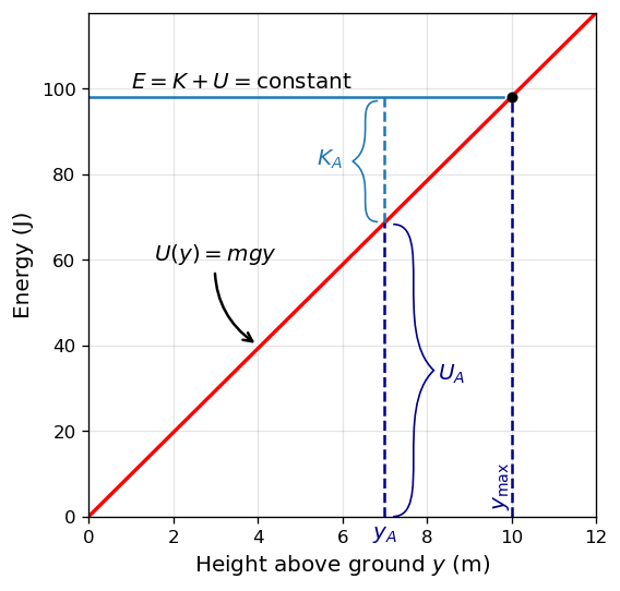
The line at energy \(E=98.1\ \mathrm{J}\) represents the constant mechanical energy of the object, whereas the kinetic (\(K_A\)) and potential (\(U_A\)) energies are indicated at a particular height \(y_A\). The total energy is divided between kinetic and potential energy as the object’s height changes.
There is a maximum potential energy and a maximum height, which an object with the given total energy cannot exceed:
If we use gravitational potential energy reference at \(y = 0\) (or \(U(0)=0\)), we can rewrite the gravitational potential energy \(U\) as \(mgy\). Solving for \(y\) gives
At the maximum height, the kinetic energy (and speed) are zero. If the object were initially traveling upward, its velocity would go to zero and \(y_{\rm max}\) would be a turning point in the motion.
At ground level, \(y_o = 0\), the potential energy is zero and the kinetic energy is maximized:
The maximum speed \(\pm v_o\) gives the initial velocity necessary to reach the maximum height \(y_{\rm max}\), and \(-v_o\) represents the final velocity after falling from \(y_{\rm max}\).
8.4.2. Potential Energy of a Spring#
Consider a mass-spring system (Fig. 8.5) on a frictionless, stationary, horizontal surface, so that gravity and the normal contact force do no work and can be ignored.
This is like a 1D system whose mechanical energy \(E\) is a constant and whose potential energy \(U(x) = \frac{1}{2}kx^2\) with respect to zero energy at zero displacement from the spring’s unstretched length \(x=0\).
Fig. 8.5 A glider between springs on an air track is an example of a horizontal mass-spring system. The potential energy diagram shows how the total mechanical energy sets the turning points, while the slope of \(U(x)\) determines the force direction. Image Credit: OpenStax: Potential Energy Diagrams and Stability.#
You can deduce the physically allowable range of motion, as well as, the maximum values of distance and speed from the limits on the kinetic energy (\(0\leq K \leq E\)). We can find two turning points when \(K=0\) and \(U=E\) for the elastic spring potential energy,
The glider’s motion (in Fig. 8.5a) is confined to the region between the turning points, \(-x_{\rm max} \leq x \leq x_{\rm max}\). This is true for any (positive) value of \(E\) because the potential energy is unbounded with respect to \(x\).
For this reason, \(U(x)\) is called an infinite potential well. At the bottom of the potential well \(x=0\) and \(U=0\), while the kinetic energy is a maximum \(K=E\) and \(v_{\rm max} = \pm \sqrt{\frac{2E}{m}}\).
From the slop of this potential energy curve (Fig. 8.5b), you can deduce information about the force on the glider and its acceleration.
The slope, force, and acceleration are all zero when \(x=0\), so this is an equilibrium point.
The negative of the slope (on either side of the equilibrium point) gives a force pointing back to the equilibrium point (i.e., \(F=\pm kx\)), so the equilibrium is termed stable and the force is called a restoring force.
If the force on either side of an equilibrium point has a direction that is the same as the direction of position change (i.e., pointing away from the equilibrium point), the equilibrium is termed unstable.
A stable point occurs when \(U(x)\) has a relative minimum, while an unstable point occurs when \(U(x)\) ahs a relative maximum. This should be intuitive because a ball rolls downhill into a valley.
8.4.3. Example Problem: Quartic and Quadratic Potential Energy Diagram#
Exercise 8.10
The Problem
The potential energy for a particle undergoing one-dimensional motion along the \(x\)-axis is \(U(x) = 2\left(x^4-x^2\right)\), where \(U\) is in joules and \(x\) is in meters. The particle is not subject to any non-conservative forces and its mechanical energy is constant at \(E = -0.25\ \mathrm{J}\). (a) Is the motion of the particle confined to any regions on the \(x\)-axis, and if so, what are they? (b) Are there any equilibrium points, and if so, where are they and are they stable or unstable?
Show worked solution
The Model
The system consists of the particle moving along the \(x\)-axis under a conservative force derived from the given potential energy function. No non-conservative forces act, so the mechanical energy \(E\) is constant. The motion is only allowed where the kinetic energy satisfies \(K = E - U(x) \ge 0\), which is equivalent to \(U(x) \le E\). Equilibrium points occur where the net force is zero, which for a one-dimensional conservative system means \(F_x = -dU/dx = 0\). Stability is determined from the shape of \(U(x)\) near the equilibrium point: a relative minimum corresponds to stable equilibrium and a relative maximum corresponds to unstable equilibrium.
The Math
(a) The motion is allowed where \(K = E - U(x) \ge 0\), so
Rearranging and completing the square in \(x^2\) gives
Dividing by \(2\) and taking square roots yields the condition on \(x^2\),
Therefore the motion is confined to two symmetric intervals,
where
(b) Equilibrium points occur where \(F_x = -dU/dx = 0\), which is equivalent to \(dU/dx = 0\). Differentiating \(U(x)=2(x^4-x^2)\) gives
Setting this equal to zero yields
Stability is determined from the second derivative,
Evaluating at the equilibrium points gives
The Conclusion
The particle’s motion is confined to two allowed regions where \(U(x) \le E\), namely \(x_P \le x \le x_R\) and \(-x_R \le x \le -x_P\), with \(x_P \approx 0.38\ \mathrm{m}\) and \(x_R \approx 0.92\ \mathrm{m}\). The equilibrium points are at \(x=0\) and \(x=\pm 1/\sqrt{2}\); the equilibrium at \(x=0\) is unstable, while the equilibria at \(x=\pm 1/\sqrt{2}\) are stable.
The Verification
The python code belows verifies the solution by generating a plot of the potential and labeling the equilibria.
Show code cell source
import numpy as np
import matplotlib.pyplot as plt
# ----- parameters -----
E = -0.25
def U(x):
return 2*(x**4 - x**2)
# Turning points from the analytic x^2 bounds
xP = np.sqrt(0.5 - np.sqrt(1/8))
xR = np.sqrt(0.5 + np.sqrt(1/8))
# Equilibria
xQ = 1/np.sqrt(2)
# ----- make figure -----
fs = 'large'
x = np.linspace(-1.25, 1.25, 1200)
Ux = U(x)
fig = plt.figure(figsize=(8, 5.2), dpi=140)
ax = fig.add_subplot(111)
# Grid
ax.grid(True, alpha=0.15, color='k')
# Potential curve
ax.plot(x, Ux, lw=2,color='k',zorder=2)
# Energy line E
ax.axhline(E, ls='--', lw=1.8)
ax.text(0.02, E-0.045, r'$E=-0.25$', fontsize=fs)
# Mark turning points where U(x)=E
turn_pts = np.array([-xR, -xP, xP, xR])
ax.plot(turn_pts, U(turn_pts), 'ko', ms=5)
# Mark equilibria (critical points)
eq_pts = np.array([-xQ, 0.0, xQ])
ax.plot(eq_pts, U(eq_pts), 'ko', ms=5)
# Dashed vertical guides
for xp in [-xR, -xP, xP, xR, -xQ, xQ]:
ax.plot([xp, xp], [0, E], ls='--', lw=2, alpha=0.6)
# Labels near key x-positions
ax.text(-xR, 0.03, r'$-R$', ha='center', fontsize=fs)
ax.text(-xQ, 0.03, r'$-Q$', ha='center', fontsize=fs)
ax.text(-xP, 0.03, r'$-P$', ha='center', fontsize=fs)
ax.text(xP, 0.03, r'$P$', ha='center', fontsize=fs)
ax.text(xQ, 0.03, r'$Q$', ha='center', fontsize=fs)
ax.text(xR, 0.03, r'$R$', ha='center', fontsize=fs)
# Function label with arrow
ax.annotate(r'$U(x)=2(x^4-x^2)$', xy=(-1.02, U(-1.02)), xytext=(-0.85, 0.25), fontsize=fs,
arrowprops=dict(arrowstyle='->', lw=1.4, connectionstyle='arc3,rad=0.25'))
# Axes centered (inline axes)
ax.spines['left'].set_position('zero')
ax.spines['bottom'].set_position('zero')
ax.spines['right'].set_color('none')
ax.spines['top'].set_color('none')
ax.xaxis.set_ticks_position('bottom')
ax.yaxis.set_ticks_position('left')
# Limits and labels
ax.minorticks_on()
ax.tick_params(which='both',axis='both',length=4,width=2)
ax.set_xlim(-1.2, 1.2)
ax.set_ylim(-0.55, 0.55)
ax.text(1.05,0.02,'$\mathbf{x\ ({\\rm m})}$',horizontalalignment='left',fontsize=fs)
ax.text(-0.1,0.48,'$\mathbf{U\ ({\\rm J})}$',horizontalalignment='left',fontsize=fs,rotation=90)
# ax.set_xlabel('$x\ \mathrm{(m)}$', fontsize=fs)
# ax.set_ylabel('$U\ \mathrm{(J)}$', fontsize=fs, rotation=0, labelpad=18)
ax.set_xticks([-1,-0.5,0,0.5,1])
ax.set_xticklabels(['-1.0','-0.5','','0.5','1.0'])
ax.set_yticks([-0.4,-0.2,0,0.2,0.4])
ax.set_yticklabels(['-0.4','-0.2','','0.2','0.4'])
plt.show()
print("x_P = %.3f m, x_R = %.3f m" % (xP, xR))
print("U(x_P) = %.3f J, U(x_R) = %.3f J (should both equal E = %.2f J)" % (U(xP), U(xR), E))
print("Equilibria at x = 0 and x = ±1/sqrt(2) = ±%.3f m" % xQ)
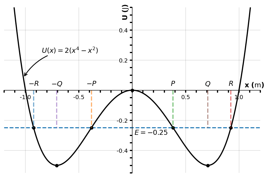
x_P = 0.383 m, x_R = 0.924 m
U(x_P) = -0.250 J, U(x_R) = -0.250 J (should both equal E = -0.25 J)
Equilibria at x = 0 and x = ±1/sqrt(2) = ±0.707 m
8.4.4. Example Problem: Sinusoidal Oscillations#
Exercise 8.11
The Problem
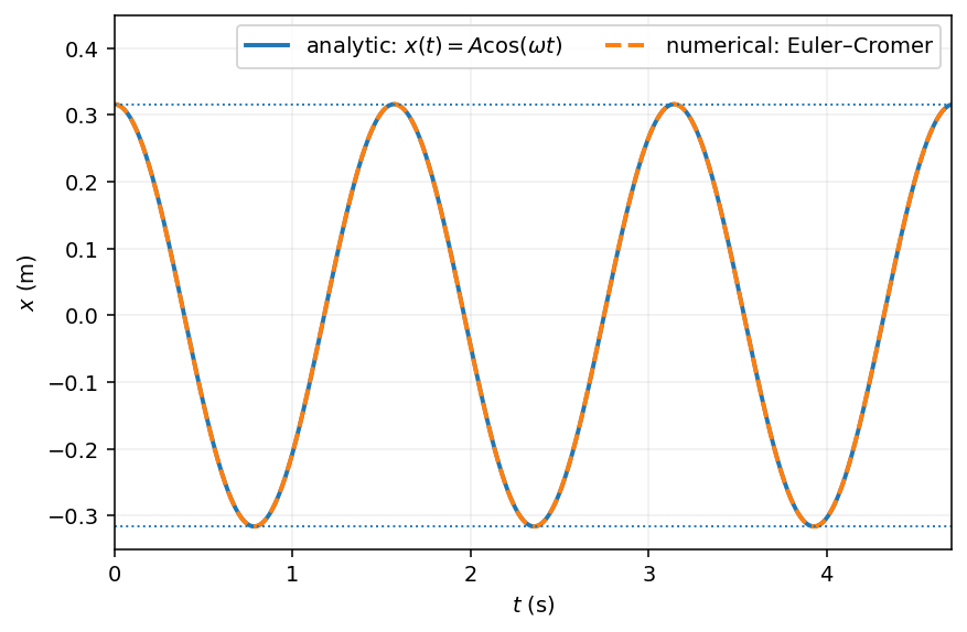
Find \(x(t)\) for a particle moving with a constant mechanical energy \(E>0\) and a potential energy \(U(x)=\tfrac{1}{2}kx^2\), when the particle starts from rest at time \(t=0\).
Show worked solution
The Model
The particle undergoes one-dimensional motion along the \(x\)-axis under a conservative force derived from the quadratic potential energy \(U(x)=\tfrac{1}{2}kx^2\). No non-conservative forces act, so the mechanical energy \(E=K+U\) is conserved. The particle is released from rest, which means its initial kinetic energy is zero and all of the mechanical energy is initially stored as potential energy. The motion is therefore bounded between turning points where the kinetic energy vanishes and the potential energy equals the total energy.
The Math
We begin from the energy-based equation of motion for one-dimensional conservative systems,
Substituting \(U(x)=\tfrac{1}{2}kx^2\) gives
Factoring out the constants allows the integral to be written as
Evaluating this standard integral yields
The particle starts from rest at \(t=0\), so the initial kinetic energy is zero and the initial potential energy satisfies \(\tfrac{1}{2}kx_o^2=E\). This implies \(x_o/\sqrt{2E/k}=\pm 1\), and therefore \(\sin^{-1}(\pm 1)=\pm 90^\circ\). Solving the previous expression for \(x\) gives
Using the trigonometric identity \(\sin(\theta\pm 90^\circ)=\pm\cos\theta\), the position can be written in the more familiar form
The Conclusion
The particle executes sinusoidal motion with position
where the amplitude is \(\sqrt{2E/k}\) and the angular frequency is \(\sqrt{k/m}\). The motion is periodic and bounded between the turning points where the kinetic energy vanishes.
The Verification
The result is consistent with the standard solution for a mass–spring system undergoing simple harmonic motion, where the force is linear in displacement and the acceleration is proportional to \(-x\). The cosine dependence reflects the fact that the particle is released from rest at a turning point, with all of its energy initially stored as potential energy.
import numpy as np
import matplotlib.pyplot as plt
# ----- choose numerical values for a check -----
m = 0.50 # kg
k = 8.0 # N/m
E = 0.40 # J (must be > 0)
omega = np.sqrt(k/m)
A = np.sqrt(2*E/k) # amplitude from E = (1/2)kA^2
# Initial conditions: released from rest at a turning point
x0 = A
v0 = 0.0
# ----- time grid -----
T = 2*np.pi/omega
t_end = 3*T
dt = T/2000
t = np.arange(0, t_end + dt, dt)
# ----- analytic solution -----
x_analytic = A*np.cos(omega*t)
# ----- numerical solution (Euler–Cromer) -----
x_num = np.zeros_like(t)
v_num = np.zeros_like(t)
x_num[0] = x0
v_num[0] = v0
for i in range(len(t)-1):
a = -(k/m)*x_num[i]
v_num[i+1] = v_num[i] + a*dt
x_num[i+1] = x_num[i] + v_num[i+1]*dt
# ----- plot comparison -----
fig = plt.figure(figsize=(7,4.5), dpi=140)
ax = fig.add_subplot(111)
ax.plot(t, x_analytic, lw=2, label='analytic: $x(t)=A\\cos(\\omega t)$')
ax.plot(t, x_num, ls='--', lw=2, label='numerical: Euler–Cromer')
ax.axhline(A, ls=':', lw=1)
ax.axhline(-A, ls=':', lw=1)
ax.set_xlabel('$t$ (s)')
ax.set_ylabel('$x$ (m)')
ax.set_xlim(0,4.7)
ax.set_ylim(-0.35,0.45)
ax.grid(True, alpha=0.2)
ax.legend(loc='best',ncols=2)
plt.show()
8.5. Sources of Energy#
Energy can take different forms and can be transferred from one form to another. Many situations are best understood (or more easily conceptualized) by considering energy. So far, no experimental results have contradicted the conservation of energy. Whenever measurements have appeared to conflict with energy conservation, new forms of energy have been discovered or recognized.
What are some other forms of energy?
Atoms and molecules inside all objects are in random motion. The internal kinetic energy form these motions is called thermal energy because it is related to the temperature of the object (i.e., heat energy).
Electrical energy is a common form that is converted to many other forms and does work in a wide range of practical situations.
Fuels (e.g., gasoline and food) have chemical energy, which is potential energy arising from their molecular bonds.
Chemical energy can be converted into thermal energy by reactions like oxidation.
Chemical reactions can also produce electrical energy (e.g., batteries).
Electrical energy can produce thermal energy (e.g., electric heater) and light (e.g., a light bulb).
Light is radiant energy, which can include radio, infrared (IR), visible, ultraviolet (UV), X-rays, and gamma rays. All bodies with thermal energy can radiate energy in electromagnetic waves.
Nuclear energy results from measurable amounts of mass converted into energy.
The Sun transforms nuclear energy into radiant energy.
Nuclear power plants use the thermal energy produced by the reactions to boil water, which is turned into electrical energy by generators.
All forms of energy can be transformed into one another and can be converted into mechanical work albeit imperfectly.
The transformation of energy from one form to another happens all the time. The chemical energy in food is converted into thermal energy through metabolism (or respiration), where light energy is converted into chemical energy through photosynthesis.
Energy conversion occurs in a solar cell. Sunlight delivers radiant energy to the cell, which causes the electrons to do work by moving and moving electrons is electricity. This electricity can be used in electric motors or heat water.
Many other sources (e.g., coal, natural gas, wood) transform their chemical energy into thermal energy which is used to transform water into steam in a boiler. Some of the energy from the steam is converted to mechanical energy when it pushes and spins a turbine, which is connected to a generator to produce electrical energy.
Not all of the initial energy is converted because some energy is transferred to the environment. No such thing as a free lunch is a common phrase to summarize the 1st and 2nd laws of thermodynamics.
8.6. In-class Problems#
8.6.1. Part I#
Problem 1
A force \(F(x) = (3.0/x^2)\ \mathrm{N}\) acts on a particle as it moves along the positive \(x\)-axis.
(a) How much work does the force do on the particle as it moves from \(x = 2.0\ \mathrm{m}\) to \(x = 5.0\ \mathrm{m}\)?
(b) Picking a convenient reference point of the potential energy to be zero at \(x = \infty\), find the potential energy for this force.
Problem 2
In the movie Monty Python and the Holy Grail a cow is catapulted from the top of a castle wall over to the people down below. The gravitational potential energy is set to zero at ground level. The cow is launched from a spring of spring constant \(1.1 \times 10^{4}\ \mathrm{N/m}\) that is expanded \(0.5\ \mathrm{m}\) from equilibrium. If the castle is \(9.1\ \mathrm{m}\) tall and the mass of the cow is \(110\ \mathrm{kg}\),
(a) what is the gravitational potential energy of the cow at the top of the castle?
(b) What is the elastic spring energy of the cow before the catapult is released?
(c) What is the speed of the cow right before it lands on the ground?
Problem 3
A particle of mass \(2.0\ \mathrm{kg}\) moves under the influence of the force \(F(x) = (-5x^2 + 7x)\ \mathrm{N}\). If its speed at \(x = -4.0\ \mathrm{m}\) is \(v = 20.0\ \mathrm{m/s}\), what is its speed at \(x = 4.0\ \mathrm{m}\)?
8.6.2. Part II#
Problem 4
Using energy considerations and assuming negligible air resistance, show that a rock thrown from a bridge \(20.0\ \mathrm{m}\) above water with an initial speed of \(15.0\ \mathrm{m/s}\) strikes the water with a speed of \(24.8\ \mathrm{m/s}\) independent of the direction thrown. (Hint: show that \(K_i + U_i = K_f + U_f\).)
Problem 5
A small block of mass \(m\) slides without friction around the loop-the-loop apparatus shown.
(a) If the block starts from rest at \(A\), what is its speed at \(B\)?
(b) What is the force of the track on the block at \(B\)?
Fig. 8.6 Image Credit: OpenStax: Chapter 8 Problems.#
Problem 6
A particle of mass \(4.0\ \mathrm{kg}\) is constrained to move along the \(x\)-axis under a single force \(F(x) = -cx^3\), where \(c = 8.0\ \mathrm{N/m^3}\). The particle’s speed at \(A\), where \(x_A = 1.0\ \mathrm{m}\), is \(6.0\ \mathrm{m/s}\). What is its speed at \(B\), where \(x_B = -2.0\ \mathrm{m}\)?
8.7. Homework#
8.7.1. Conceptual Problems#
Problem 1
What is the dominant factor that affects the speed of an object that started from rest down a frictionless incline if the only work done on the object is from gravitational forces?
Problem 2
Neglecting air resistance, how much would I have to raise the vertical height if I wanted to double the impact speed of a falling object?
8.7.2. Numerical Problems#
Problem 3
A camera weighing \(10\ \mathrm{N}\) falls from a small drone hovering \(20\ \mathrm{m}\) above the ground and enters free fall.
(a) What is the change in gravitational potential energy of the camera as it falls from the drone to the ground if the ground is chosen as the zero reference level?
(b) What is the change in gravitational potential energy if the drone is chosen as the zero reference level?
If the zero reference level is instead chosen to be a person standing \(30\ \mathrm{m}\) above the ground:
(c) What is the gravitational potential energy of the camera just before it falls?
(d) What is the gravitational potential energy of the camera after it lands on the ground?
Problem 4
Find the force corresponding to the potential energy \(U(x) = -a/x + b/x^2\).
Problem 5
Tarzan grabs a vine hanging vertically from a tall tree when he is running at \(9.0\ \mathrm{m/s}\).
(a) How high can he swing upward?
(b) Does the length of the vine affect this height?
Problem 6
A \(4.0\text{-kg}\) particle moving along the \(x\)-axis is acted upon by the force whose functional form appears below. The velocity of the particle at \(x = 0\) is \(v = 6.0\ \mathrm{m/s}\). Find the particle’s speed at
(a) \(x = 2.0\ \mathrm{m}\),
(b) \(x = 4.0\ \mathrm{m}\),
(c) \(x = 10.0\ \mathrm{m}\).
(d) Does the particle turn around at some point and head back toward the origin?
(e) Repeat part (d) if \(v = 2.0\ \mathrm{m/s}\) at \(x = 0\).
Fig. 8.7 Image Credit: OpenStax: Chapter 8 Problems.#