9. Linear Momentum and Collisions#
Jul 20, 2026 | 12366 words | 82 min read
Chapter roadmap
This chapter develops momentum as a tool for analyzing short interactions, collisions, explosions, and systems whose mass can change. As you read, focus on three questions:
How does impulse connect force, time, and change in momentum?
When is momentum conserved for a chosen system?
How do center of mass and rocket propulsion extend the same momentum ideas to more complex systems?
Keep asking what system is being analyzed and whether external impulses can be ignored.
9.1. Linear Momentum#
When using kinetic energy, we see that an object’s motion can be described by combining its mass \(m\) and velocity squared \(v^2\) into a scalar. However, we can also include the direction of motion into a description that combines mass and velocity \(\vec{\rm v}\) as a vector.
Like kinetic energy, this quantity is a way of characterizing the “quantity of motion” for an object. Momentum (from the Latin word movimentum, meaning movement) is represented by the letter \(p\)
Momentum
The momentum \(p\) of an object is the product of its mass and its velocity:
Momentum is a vector quantity, which is a property it inherits from the velocity. The momentum is most useful when determining whether an object’s motion is difficult to change or easy to change over a short time interval.
Unlike kinetic energy, momentum depends equally on an object’s mass and velocity. The average speed of an air molecule at room temperature is \({\sim}500\ {\rm m/s}\), with an average molecular mass of \(6\times 10^{-25}\ {\rm kg}\), and thus, its momentum is given by
For comparison, a typical automobile might have a speed of only \(15\ {\rm m/s}\), but a mass of \(1400\ {\rm kg}\), which gives it a momentum of
These momenta are different by 27 orders of magnitude!
9.2. Impulse and Collisions#
If an object’s velocity should change (due to the application of a force), then its momentum changes as well. This indicates a connection between momentum and force.
Suppose you apply a force \(F\) on a free object over a time interval \(\Delta t\).
An increase in force will result in a proportional increase in the change of momentum.
A larger time spent applying a force will result in a proportional increase in the change of momentum.
A change in an object’s motion can be proportional to the magnitude of the force and to the time interval over which the force is applied.
Mathematically, if a quantity is proportional to two quantities, then it is proportional to their product. The product of a force and a time interval is called impulse, which is represented by \(\vec{J}\) and has units of \({\rm N\cdot s}\).
Impulse
Let \(\vec{F}(t)\) be the force applied to an object over some differential time interval \(dt\). The resulting impulse on the object is defined as
The total impulse over the interval \(t_f-t_i\) is given by
When a force is applied for an infinitesimal time interval \(dt\), then it causes an infinitesimal impulse \(d\vec{J}\), and the total impulse is the sum over all of these infinitesimal impulses.
To calculate the impulse, we need to know the force function \(F(t)\) (which we often don’t). However, we can use a result from calculus called a mean value theorem or
Applying this to the time-dependent force function, we find
which we can rewrite in terms of the impulse as
Note
You can calculate the impulse on the object even if you don’t know the details of the force as a function of time; you only need the average force.
You usually determine the impulse (by measurement or calculation) and then calculate the average force that caused that impulse. To calculate the impulse, we can start from a version of Newton’s 2nd law:
For a constant force \(\vec{F}_{\rm ave} = \vec{F} = m\vec{a}\), which simplifies to
Checkpoint
If the same impulse is delivered over a longer time interval, what happens to the average force?
Momentum changes when an object experiences an impulse. As you watch, focus on how the same change in momentum can come from a large force over a short time or a smaller force over a longer time. This idea explains why collision time matters in crashes, sports impacts, and safety equipment.
9.2.1. Example Problem: Arizona Meteor Crater#
Exercise 9.1
The Problem
Approximately \(50{,}000\) years ago, a large (radius of \(25\ {\rm m}\)) iron-nickel meteorite collided with Earth at an estimated speed of \(1.28\times 10^4\ {\rm m/s}\) in what is now the northern Arizona desert, in the United States. The impact produced a crater that is still visible today; it is approximately \(1200\ {\rm m}\) (three-quarters of a mile) in diameter, \(170\ {\rm m}\) deep, and has a rim that rises \(45\ {\rm m}\) above the surrounding desert plain. Iron-nickel meteorites typically have a density of \(\rho = 7970\ {\rm kg/m^3}\). Use impulse considerations to estimate the average force and the maximum force that the meteor applied to Earth during the impact.
Show worked solution
The Model
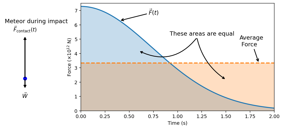
The system consists of the meteor during the short collision interval with Earth. We model the meteor as a uniform-density sphere of radius \(R\) and density \(\rho\), moving vertically just before impact. We define upward as the \(+y\) direction and use \(\hat{j}\) as the upward unit vector. Immediately before impact, the meteor’s velocity is downward, so its initial velocity has a negative \(y\)-component. During the collision interval \(\Delta t\), the meteor is brought to rest by a large upward contact force exerted by Earth. The meteor’s weight acts downward, but during the extremely short impact interval the contact force is assumed to be much larger than the weight, so the momentum change is dominated by the contact interaction.
Because we want to know the average force, we replace the true time-varying contact force with an effective constant force acting over the interval \(\Delta t\) that produces the same change in momentum. The impulse on the meteor therefore points in the direction of \(\Delta \vec{\rm v}\), which is upward since the meteor’s downward velocity is reduced to zero. To estimate the maximum force, we must assume a time-dependence for the contact force during impact. We model the force magnitude as a rapidly decaying function of time that begins near a maximum value and decreases toward zero by the end of the collision interval. This assumed force profile is chosen so that its time-average matches the previously determined average force.
By Newton’s 3rd law, the force the meteor applies to Earth is equal in magnitude and opposite in direction to the force Earth applies to the meteor. The analysis therefore depends only on the meteor’s change in momentum during the collision interval and not on the depth to which it penetrates the ground.
The Math
The impact force is related to impulse because the net impulse equals the change in momentum. The system requires a change in momentum to bring the meteor from its initial velocity to rest, given by the impulse–momentum theorem.
For a short impact, the impulse on the meteor is \(\vec{J} = m\,\Delta \vec{\rm v}.\)
The meteor is moving downward initially and stops after impact. Using the \(+y\) direction as upward, we write the initial and final velocities as
The change in velocity is therefore upward: \(\Delta \vec{\rm v} = \vec{\rm v}_f - \vec{\rm v}_i = v_o\,\hat{j}.\)
The average net force during impact is the impulse divided by the impact duration, \(J/\Delta t\). For an approximately constant average force over \(\Delta t\), the average force on the meteor is
The mass is determined from density and volume. For a spherical meteor, the mass is
which allows us to calculate the average force as
Using the given values and the estimate \(\Delta t = 2\ {\rm s}\) yields
Using Newton’s 3rd law, the meteor applies an equal-magnitude force to Earth in the opposite direction, so the average force applied to Earth is downward with magnitude \(\left|\vec{F}_{\rm ave}\right|\).
To estimate the maximum force, we choose a simple rapidly-decaying force function (e.g., \(F \propto e^{-kt^2}\)) that starts near a maximum and decreases toward zero during the impact. We model the contact force on the meteor as
The average force over the interval is the time-average of this function. The system requires the time-average of \(\vec{F}(t)\) to match \(\vec{F}_{\rm ave}\), given by
Because the force always points in \(+\hat{j}\) during impact, we equate magnitudes:
We choose \(\tau=\Delta t/e\) to represent a force that decays substantially over the impact duration. We solve this expression for \(F_{\max}\), which yields
With \(\Delta t=2\ {\rm s}\), the time-average factor evaluates to
which sets the timescale so that the force has decayed significantly by the end of the collision interval. The maximum force magnitude is
The Conclusion
Modeling the meteor as a uniform sphere of radius \(25\ {\rm m}\) and density \(7970\ {\rm kg/m^3}\) gives a mass of \(5.21\times 10^8\ {\rm kg}\). If the meteor is brought from \(1.28\times 10^4\ {\rm m/s}\) to rest in \(\Delta t=2\ {\rm s}\), the average impact force magnitude is \(3.33\times 10^{12}\ {\rm N}\). By Newton’s 3rd law, the average force the meteor applied to Earth is the same magnitude downward.
Using a decaying-force model with \(\tau=\Delta t/e\) gives a maximum force magnitude of \(7.27\times 10^{12}\ {\rm N}\), so the maximum force the meteor applied to Earth is also downward with this magnitude. These values are estimates because the impact time and the detailed force–time profile are idealizations of a complex event.
The Verification
We verify the mass, impulse, average force, and the time-average factor numerically using NumPy. We also generate a free-body diagram for the meteor during impact using draw_fbd and an impulse plot showing that the area under \(F(t)\) matches the rectangle area \(F_{\rm ave}\Delta t\).
import numpy as np
# ---------------- given values ----------------
rho = 7970.0 # kg/m^3
R = 25.0 # m
v0 = 1.28e4 # m/s
dt = 2.0 # s
# ---------------- mass, impulse, average force ----------------
V = (4.0/3.0)*np.pi*R**3
m = rho*V
J = m*v0
F_ave = J/dt
# ---------------- maximum force model ----------------
tau = dt/np.e
t = np.arange(0.0, dt+0.001, 0.001)
shape = np.exp(-t**2/(2.0*tau**2))
avg_shape = (1.0/dt)*np.trapz(shape, t)
F_max = F_ave/avg_shape
F_t = F_max*shape
# ---------------- impulse check ----------------
J_model = np.trapz(F_t, t)
J_rect = F_ave*dt
# ---------------- rounding before printing ----------------
m_r = float(f"{m:.3e}")
J_r = float(f"{J:.3e}")
Fave_r = float(f"{F_ave:.3e}")
avgshape_r = round(float(avg_shape), 3)
Fmax_r = float(f"{F_max:.3e}")
Jmodel_r = float(f"{J_model:.3e}")
Jrect_r = float(f"{J_rect:.3e}")
print(f"The meteor mass is {m_r:.3e} kg.")
print(f"The impulse magnitude is {J_r:.3e} N*s.")
print(f"Using tau = dt/e gives tau = {tau:.3f} s.")
print(f"The average impact force magnitude is {Fave_r:.3e} N.")
print(f"The time-average factor is {avgshape_r:.3f}.")
print(f"The maximum force magnitude is {Fmax_r:.3e} N.")
print(f"The impulse from the force model is {Jmodel_r:.3e} N*s.")
print(f"The rectangle impulse F_ave*dt is {Jrect_r:.3e} N*s.")
Show code cell source
import numpy as np
import matplotlib.pyplot as plt
from matplotlib.gridspec import GridSpec
# ---------------- given values ----------------
rho = 7970.0 # kg/m^3
R = 25.0 # m
v0 = 1.28e4 # m/s
dt = 2.0 # s
# ---------------- mass, impulse, average force ----------------
V = (4.0/3.0)*np.pi*R**3
m = rho*V
J = m*v0
F_ave = J/dt
# ---------------- maximum force model ----------------
tau = dt/np.e
t = np.arange(0.0, dt+0.0001, 0.0001)
shape = np.exp(-t**2/(2.0*tau**2))
if hasattr(np, "trapezoid"):
integral_shape = np.trapezoid(shape, t) # integral of the dimensionless force-shape curve
else:
integral_shape = np.trapz(shape, t) # integral of the dimensionless force-shape curve
avg_shape = integral_shape / dt # time-average factor for the force model
F_max = F_ave / avg_shape # maximum force magnitude (N)
F_t = F_max * shape # force as a function of time (N)
if hasattr(np, "trapezoid"):
J_model = np.trapezoid(F_t, t) # impulse from the modeled force curve (N*s)
else:
J_model = np.trapz(F_t, t) # impulse from the modeled force curve (N*s)
J_rect = F_ave * dt # impulse from the average-force rectangle (N*s)
# ---------------- rounding before printing ----------------
m_r = float(f"{m:.3e}")
J_r = float(f"{J:.3e}")
Fave_r = float(f"{F_ave:.3e}")
avgshape_r = round(float(avg_shape), 3)
Fmax_r = float(f"{F_max:.3e}")
Jmodel_r = float(f"{J_model:.3e}")
Jrect_r = float(f"{J_rect:.3e}")
print(f"The meteor mass is {m_r:.3e} kg.")
print(f"The impulse magnitude is {J_r:.3e} N*s.")
print(f"Using tau = dt/e gives tau = {tau:.3f} s.")
print(f"The average impact force magnitude is {Fave_r:.3e} N.")
print(f"The time-average factor is {avgshape_r:.3f}.")
print(f"The maximum force magnitude is {Fmax_r:.3e} N.")
print(f"The impulse from the force model is {Jmodel_r:.3e} N*s.")
print(f"The rectangle impulse F_ave*dt is {Jrect_r:.3e} N*s.")
def draw_fbd(ax, forces, labels=None, note="", title=None):
ax.plot(0., 0.0, "bo", markersize=7)
if labels is None:
labels = [""]*len(forces)
for F, lab in zip(forces, labels):
Fx, Fy = F[0], F[1]
ax.annotate("", xy=(Fx, Fy), xytext=(0.0, 0.0), arrowprops=dict(arrowstyle="->", lw=2))
if abs(Fx) > abs(Fy):
xlab = Fx + 0.2*np.sign(Fx)
ylab = Fy
ha, va = "center", "center"
else:
xlab = Fx
ylab = Fy + 0.15*np.sign(Fy)
ha, va = "center", "center"
ax.text(xlab, ylab, lab, fontsize=11, horizontalalignment=ha, verticalalignment=va)
ax.set_aspect("equal", adjustable="box")
ax.set_xticks([])
ax.set_yticks([])
for spine in ax.spines.values():
spine.set_visible(False)
if title is not None:
ax.set_title(title)
if note is not None and note != "":
ax.text(0.02, 0.95, note, transform=ax.transAxes, fontsize=12, va="top")
ax.set_xlim(-0.5, 1)
ax.set_ylim(-0.5, 1.5)
# ---------------- figures: FBD and impulse plot ----------------
fig = plt.figure(figsize=(10, 4), dpi=140)
gs = GridSpec(1, 2, width_ratios=[1, 3]) # right panel wider
ax1 = fig.add_subplot(gs[0])
ax2 = fig.add_subplot(gs[1])
# (1) Free-body diagram (meteor during impact)
ax1.set_xticks([])
ax1.set_yticks([])
# Contact force dominates during impact; weight is shown qualitatively smaller.
forces = [(0.0, +1.0), (0.0, -0.25)]
labels = [r'$\vec{F}_{\rm contact}(t)$', r'$\vec{W}$']
draw_fbd(ax1, forces=forces, labels=labels, note="Meteor during impact", title=None)
F_t /= 1e12
F_ave /= 1e12
ax2.plot(t, F_t, linewidth=2)
ax2.plot([0, dt], [F_ave, F_ave], linestyle='--', linewidth=2)
ax2.fill_between(t, 0.0, F_t, alpha=0.25)
ax2.fill_between([0, dt], [0.0, 0.0], [F_ave, F_ave], alpha=0.25)
# --- annotations (OpenStax-style callouts) ---
# Label the force curve F(t)
t_curve = 0.2*dt
ax2.annotate(r'$\vec{F}(t)$', xy=(t_curve, np.interp(t_curve, t, F_t)), xytext=(0.35*dt, 0.92*np.max(F_t)),
arrowprops=dict(arrowstyle='->', lw=1.5), fontsize=12)
# Label the average force line
ax2.annotate('Average\n Force', xy=(0.92*dt, F_ave), xytext=(0.82*dt, 1.35*F_ave),
arrowprops=dict(arrowstyle='->', lw=1.5), fontsize=12)
# "These areas are equal" pointing to both shaded regions
x_left = 0.30*dt
y_left = 0.8*np.interp(x_left, t, F_t)
x_right = 0.75*dt
y_right = 0.65*F_ave
ax2.text(0.46*dt, 0.72*np.max(F_t), 'These areas are equal', fontsize=12)
ax2.annotate('', xy=(x_left, y_left), xytext=(0.60*dt, 0.70*np.max(F_t)),
arrowprops=dict(arrowstyle='->', lw=1.5,connectionstyle="arc3,rad=-0.4"))
ax2.annotate('', xy=(x_right, y_right), xytext=(0.60*dt, 0.70*np.max(F_t)),
arrowprops=dict(arrowstyle='->', lw=1.5,connectionstyle="arc3,rad=0.2"))
ax2.set_xlabel("Time (s)")
ax2.set_ylabel("Force ($\\times 10^{12}$ N)")
ax2.set_xlim(0, dt)
ax2.set_ylim(0,7.5)
fig.subplots_adjust(wspace=0.1)
plt.show()
The meteor mass is 5.216e+08 kg.
The impulse magnitude is 6.677e+12 N*s.
Using tau = dt/e gives tau = 0.736 s.
The average impact force magnitude is 3.338e+12 N.
The time-average factor is 0.458.
The maximum force magnitude is 7.289e+12 N.
The impulse from the force model is 6.677e+12 N*s.
The rectangle impulse F_ave*dt is 6.677e+12 N*s.
9.2.2. Example Problem: Benefits of Impulse#
Exercise 9.2
The Problem
A car traveling at \(27\ {\rm m/s}\) collides with a building. The collision with the building causes the car to come to a stop in approximately \(1\ {\rm s}\). The driver, who weighs \(860\ {\rm N}\), is protected by a combination of a variable-tension seatbelt and an airbag. The airbag and seatbelt slow his velocity, such that he comes to a stop in approximately \(2.5\ {\rm s}\).
(a) What average force does the driver experience during the collision?
(b) Without the seatbelt and airbag, his collision time (with the steering wheel) would have been approximately \(0.20\ {\rm s}\). What force would he experience in this case?
Show worked solution
The Model
The system consists of the driver during the collision interval. We model the driver as a particle moving in one dimension along \(+x\) direction.
The driver’s velocity decreases from \(v_o = 27\ {\rm m/s}\) to zero due to a horizontal contact force from the seatbelt and airbag (or, in the unrestrained case, from the steering wheel). We assume that the dominant contribution to the driver’s horizontal momentum change comes from this contact force. The vertical forces (weight and normal force from the seat) do not significantly affect the horizontal impulse during the short collision interval.
Because we want to know the average force, we treat the collision as producing an effective constant force over a time interval \(\Delta t\) that yields the correct impulse. The driver’s mass is not given directly, so it must be determined from the stated weight using \(W = mg\).
The Math
The impulse–momentum theorem relates the net impulse to the change in momentum,
If we replace the true time-varying contact force with an average force acting over the collision time \(\Delta t\), the impulse is also
Since both expressions represent the same impulse, we equate them and solve for the average force:
The driver’s mass is obtained from his weight:
Initially, the driver moves in the \(+x\) direction, so
The change in velocity is therefore \(\Delta \vec{\rm v} = \vec{\rm v}_f - \vec{\rm v}_i = -v_o\,\hat{i}.\) The expression for the average force now gives
(a) With the seatbelt and airbag, the stopping time is \(\Delta t = 2.5\ {\rm s}\). We find the average force as
(b) Without the seatbelt and airbag, the stopping time would have been \(\Delta t = 0.20\ {\rm s}\). Repeating the calculation,
The Conclusion
When the driver is restrained by a seatbelt and airbag, he comes to rest in \(2.5\ {\rm s}\) and experiences an average force of magnitude \(948\ {\rm N}\) opposite his direction of motion. Without these safety systems, stopping in only \(0.20\ {\rm s}\) requires an average force of magnitude \(1.19\times 10^4\ {\rm N}\), also opposite the direction of motion.
Although the change in momentum is the same in both cases, increasing the collision time dramatically reduces the required average force. This illustrates why safety systems are effective: they extend the stopping time and therefore reduce the force experienced by the occupant.
The Verification
We verify the driver’s mass from the given weight and compute the two average force magnitudes using the impulse–momentum relation.
import numpy as np
# ---------------- given values ----------------
W = 860.0 # driver's weight in newtons
g = 9.81 # acceleration due to gravity (m/s^2)
v0 = 27.0 # initial speed of the driver (m/s)
# ---------------- convert weight to mass ----------------
# Using W = mg to determine the driver's mass
m = W / g
# ---------------- collision times ----------------
dt_seatbelt = 2.5 # stopping time with seatbelt and airbag (s)
dt_no_restraint = 0.20 # stopping time without restraint (s)
# ---------------- compute average forces ----------------
# Using F_ave = m * v0 / dt (magnitude only)
F_seatbelt = m * v0 / dt_seatbelt
F_no_restraint = m * v0 / dt_no_restraint
# ---------------- rounded values for clean output ----------------
m_r = np.round(m, 1)
F_seatbelt_r = float(f"{F_seatbelt:.3e}")
F_no_restraint_r = float(f"{F_no_restraint:.3e}")
print(f"The driver’s mass, computed from his weight, is {m_r} kg.")
print(f"When the stopping time is 2.5 s, the average force magnitude is {F_seatbelt_r:.3e} N.")
print(f"When the stopping time is 0.20 s, the average force magnitude is {F_no_restraint_r:.3e} N.")
print("These results confirm that increasing the stopping time dramatically reduces the force experienced by the driver.")
9.2.3. Effect of Impulse#
Since an impulse is a force acting for some amount of time, it causes an object’s motion to change. This was written previously as
Because \(m\vec{\rm v}\) is the momentum of a system, \(m\Delta\vec{\rm v}\) is the change of momentum \(\Delta\vec{p}\).
Impulse-Momentum Theorem
An impulse applied to a system changes the system’s momentum, and that change of momentum is exactly equal to the impulse that was applied:
Fig. 9.1 Impulse changes momentum by the same vector amount. Image Credit: Openstax: Impulse and Collisions.#
The impulse-momentum theorem is depicted graphically in Figure 9.1. There are two crucial concepts in the impulse-momentum theorem:
Impulse is a vector quantity, where the direction of the impulse causes a completely opposite change of momentum.
An impulse does not cause momentum, rather, it causes a change in the momentum of an object. The change in momentum is calculated similar to displacement, with the initial momentum subtracted from the final momentum.
The most impulse problems require you to calculate the applied force, or the change of velocity that occurs as a result of applying an impulse.
Problem-Solving Strategy
Impulse-Momentum Theorem
Express the impulse as force times the relevant time interval.
Express the impulse as the change of momentum, usually \(m\Delta v\).
Equate these and solve for the desired quantity.
Checkpoint
When you use \(\vec{F}_{\rm ave}=\Delta\vec{p}/\Delta t\), what system is receiving the impulse?
9.2.3.1. Example Problem: Moving the Enterprise#
Exercise 9.3
The Problem
When Captain Picard commands, “Take us out,” the starship Enterprise starts from rest to a final speed of \(v_f = 7.5 \times 10^7\ {\rm m/s}\). Assuming this maneuver is completed in \(60\ {\rm s}\), what average force did the impulse engines apply to the ship? An estimate for the mass of the Enterprise is \(2 \times 10^9\ {\rm kg}\).
Show worked solution
The Model
The system consists of the starship during the acceleration interval. We model the motion as one-dimensional along the direction of thrust. The engines apply a force in this direction, producing a change in the ship’s velocity from rest to its final speed.
Because we are asked for an average force over a known time interval, we treat the true thrust as an effective constant force acting over \(\Delta t = 60\ {\rm s}\) that produces the same change in momentum. The mass of the ship is assumed constant during the maneuver.
The Math
The impulse–momentum theorem states that the net impulse on a system equals its change in momentum, \(\vec{J} = m\,\Delta \vec{\rm v}.\) If we replace the actual time-varying thrust with an average force acting over the time interval \(\Delta t\), then the impulse is also
Since both expressions represent the same impulse, we equate them:
The ship starts from rest, so
Thus the change in velocity is \(\Delta \vec{\rm v} = \vec{\rm v}_f - \vec{\rm v}_i = v_f\,\hat{i}.\) Using the given values,
The Conclusion
To accelerate the \(2 \times 10^9\ {\rm kg}\) starship from rest to \(7.5 \times 10^7\ {\rm m/s}\) in \(60\ {\rm s}\) requires an average thrust of \(2.5 \times 10^{15}\ {\rm N}.\) This corresponds to an acceleration of \(a = \frac{F}{m} = 1.25 \times 10^6\ {\rm m/s^2}.\)
That acceleration is approximately \(130{,}000\) times Earth’s gravitational acceleration. An acceleration of \(1.25 \times 10^6\ {\rm m/s^2}\) would be instantly fatal to any biological crew and would likely destroy the structural integrity of the ship itself. The only reason this scenario works in science fiction is the assumed existence of “inertial dampeners,” which would somehow cancel the internal effects of acceleration. From a classical mechanics perspective, however, the force required is unimaginably large.
The Verification
We verify the calculation numerically using the impulse–momentum relation.
import numpy as np
# ---------------- given values ----------------
m = 2.0e9 # mass of the Enterprise in kilograms
vf = 7.5e7 # final speed in m/s
dt = 60.0 # time interval in seconds
# ---------------- compute average force ----------------
# Using F_ave = m * (vf - vi) / dt, with vi = 0
F_ave = m * vf / dt
# ---------------- compute resulting acceleration ----------------
a = F_ave / m
# ---------------- formatted output ----------------
F_r = float(f"{F_ave:.3e}")
a_r = float(f"{a:.3e}")
print(f"The average thrust required is {F_r:.3e} N.")
print(f"This produces an acceleration of {a_r:.3e} m/s^2.")
print("These results confirm the impulse–momentum calculation.")
9.2.3.2. Example Problem: The iPhone Drop#
Exercise 9.4
The Problem
Apple released its iPhone 6 Plus in November 2014. Suppose the phone is dropped from a height of \(1.5\ {\rm m}\) and strikes the floor. Estimate the average force the floor exerts on the phone during the collision. Use a mass of \(0.172\ {\rm kg}\), assume the phone is dropped from rest, and assume that it does not bounce.
Show worked solution
The Model
The system consists of the phone during the short collision interval with the floor. We model the motion as one-dimensional along the vertical axis, taking upward as the \(+y\) direction.
The phone is dropped from rest at height \(h = 1.5\ {\rm m}\). Just before impact, it has a downward velocity due to gravitational acceleration. During the collision, the floor exerts a large upward contact force that brings the phone to rest. We assume the phone does not bounce, so its final velocity immediately after impact is zero.
Because we are asked for an average force, we replace the true time-varying contact force with an effective constant force acting over a short collision time \(\Delta t\). The dominant contribution to the phone’s change in vertical momentum during the collision is due to the floor’s contact force. The collision time must be estimated.
The Math
The average force during the collision is related to impulse. The impulse–momentum theorem states that the net impulse equals the change in momentum,
If we approximate the true force as an average force acting over a time interval \(\Delta t\), then
Equating these expressions gives
To evaluate \(\Delta \vec{\rm v}\), we must first determine the velocity just before impact. Using conservation of mechanical energy and defining the floor as zero potential energy,
Solving for the speed just before impact,
Using \(g = 9.81\ {\rm m/s^2}\) and \(h = 1.5\ {\rm m}\),
After impact the phone comes to rest, \(\vec{\rm v}_2 = 0.\) The change in velocity during the collision is therefore
The average force on the phone is therefore \(\vec{F}_{\rm ave} = (m v_1/\Delta t)\,\hat{j}\).
To estimate the collision time, we approximate it as the time required for the phone to travel its own length during impact. Taking a phone length of \(0.14\ {\rm m}\) and using the impact speed,
Using the numerical values,
For comparison, the phone’s weight is
The Conclusion
Dropping the \(0.172\ {\rm kg}\) phone from a height of \(1.5\ {\rm m}\) produces an impact speed of \(5.42\ {\rm m/s}\). Bringing the phone to rest in approximately \(0.026\ {\rm s}\) requires an average upward force of magnitude \(36\ {\rm N}\).
Because the phone’s weight is only \(1.69\ {\rm N}\), the impact force is more than 20 times its weight. This large force over a very short time interval explains why fragile components can fail even from seemingly modest drop heights.
The Verification
We verify the impact speed, collision time, average force, and weight numerically.
import numpy as np
# ---------------- given values ----------------
m = 0.172 # mass of the phone in kilograms
g = 9.81 # gravitational acceleration in m/s^2
h = 1.5 # drop height in meters
L = 0.14 # approximate phone length in meters
# ---------------- compute impact speed ----------------
# Using v = sqrt(2gh) from energy conservation
v1 = np.sqrt(2*g*h)
# ---------------- estimate collision time ----------------
# Approximating collision time as length / impact speed
dt = L / v1
# ---------------- compute average force ----------------
# Using F_ave = m * v1 / dt
F_ave = m * v1 / dt
# ---------------- compute weight ----------------
# Using W = mg
W = m * g
print(f"The impact speed just before hitting the floor is {v1:.2f} m/s.")
print(f"The estimated collision time is {dt:.3f} s.")
print(f"The average force exerted by the floor is {F_ave:.1f} N.")
print(f"The weight of the phone is {W:.2f} N.")
print("These results confirm that the impact force is more than twenty times the phone’s weight.")
9.2.4. Momentum and Force#
We can rewrite the average force in terms of the momentum, or
The average force applied to an object is equal to the change of the momentum that the force causes, divided by the time interval over which this change of momentum occurs.
This relationship is useful in situations where the collision time \(\Delta t\) is small, but measurable (e.g., \({\sim}0.1\ {\rm s}\) or even \(0.001\ {\rm s}\)). Car crashes, punting a football, or collisions of subatomic particles would meet this criterion.
In the limit \(\Delta t \rightarrow dt\), the force can be written as
where \(\vec{p}\) represents a continuously changing momentum.
This says that the rate of change of the system’s momentum is exactly equal to the net applied force. This is Newton’s 2nd law written in terms of momentum rather than acceleration.
If the mass of the system remains constant, we can show that
The assumption of constant mass allowed us to pull \(m\) out of the derivative. If the mass is not constant, we cannot use this form of the second law. One advantage to expressing force in terms of changing momentum is that is that it allows for the mass of the system to change, as well as the velocity.
Newton’s 2nd Law of Motion in Terms of Momentum
The net external force on a system is equal to the rate of change of the momentum of that system caused by the force:
9.2.4.1. Example Problem: A Tennis Serve#
Exercise 9.5
The Problem
During the 2007 French Open, Venus Williams hit the fastest recorded serve in a premier women’s match, reaching a speed of \(58\ {\rm m/s}\) \((209\ {\rm km/h})\). What is the average force exerted on the \(0.057\ {\rm kg}\) tennis ball by Venus Williams’ racquet? Assume that the ball’s speed just after impact is \(58\ {\rm m/s}\), that the initial horizontal component of the velocity before impact is negligible, and that the ball remained in contact with the racquet for \(5.0\ {\rm ms}\).
Show worked solution
The Model
The system consists of the tennis ball during the brief contact interval with the racquet. The interaction is modeled as 1D along the horizontal direction of the serve, because the ball’s initial horizontal velocity component is negligible and the racquet’s force acts primarily along the outgoing direction.
The racquet’s force changes the ball’s horizontal momentum from approximately zero to a final speed of \(58\ {\rm m/s}\) over a short contact time of \(\Delta t = 5.0\ {\rm ms}\). The force during contact is not constant in time, but an average force can be defined as the constant force that would produce the same change in momentum over the same time interval. The ball also experiences its weight during contact, but that force acts vertically and is small compared with the horizontal contact force being estimated.
The Math
The average net force over a time interval is related to the change in momentum by the impulse–momentum theorem written in average-force form,
The ball’s mass is constant during the collision, so the momentum change can be written in terms of the velocity change as
Since the initial horizontal component of the velocity is negligible, the initial velocity in the serve direction is approximated as \(\vec{\rm v}_i \approx 0\). The speed just after impact is \(58\ {\rm m/s}\) in the serve direction, so the final velocity can be written as \(\vec{\rm v}_f = (58\ {\rm m/s})\hat{i}\), which gives a velocity change of \(\Delta \vec{\rm v} = (58\ {\rm m/s})\hat{i}\).
The magnitude of the momentum change is then
The contact time is \(\Delta t = 5.0\ {\rm ms} = 5.0\times 10^{-3}\ {\rm s}\). The average force magnitude follows from \(\,F_{\rm ave}=\Delta p/\Delta t\),
The Conclusion
The tennis ball’s horizontal momentum changes from approximately zero to \(m(58\ {\rm m/s})\) in \(5.0\ {\rm ms}\), which requires an average force of about \(660\ {\rm N}\) from the racquet in the direction of the serve. This force is much larger than the ball’s weight (about \(0.56\ {\rm N}\)), which is why gravity has a negligible effect during the brief contact time.
A force of \(660\ {\rm N}\) corresponds to the weight of a person with a mass of about \(67\ {\rm kg}\) under Earth’s gravity. Venus Williams’ reported weight range of 159–165 lb corresponds to approximately 72–75 kg, which gives a weight of about 710–740 N. The average force on the tennis ball is therefore comparable to supporting nearly her full body weight.
The Verification
We verify the momentum change and average force numerically using NumPy, and we compare the result to the ball’s weight to confirm that gravity is negligible during contact.
import numpy as np
# ---------------- given values ----------------
m = 0.057 # Ball mass in kilograms.
vf = 58.0 # Ball speed just after impact in m/s.
vi = 0.0 # Initial horizontal component is negligible (approx. zero).
dt = 5.0e-3 # Contact time in seconds (5.0 ms).
g = 9.81 # Gravitational acceleration in m/s^2.
# ---------------- momentum change ----------------
# The change in momentum magnitude is m*(vf - vi) for one-dimensional motion.
dp = m * (vf - vi)
# ---------------- average force ----------------
# The average force magnitude is dp/dt over the contact interval.
F_ave = dp / dt
# ---------------- weight comparison ----------------
# The ball’s weight magnitude is mg, used to compare against the contact force.
W = m * g
# ---------------- formatted output ----------------
print(f"The change in momentum during contact is {dp:.2f} kg*m/s.")
print(f"The average force magnitude during contact is {F_ave:.0f} N.")
print(f"The tennis ball’s weight is {W:.2f} N, which is much smaller than the contact force.")
9.3. Conservation of Linear Momentum#
Recall Newton’s 3rd law: When two objects of masses \(m_1\) and \(m_2\) interact, the force that object 2 applies to object 1 is equal in magnitude and opposite in direction. Let
\(\vec{F}_{12} = \text{the force on }m_1\ \text{from } m_2\),
\(\vec{F}_{21} = \text{the force on }m_2\ \text{from } m_1\).
Then, Newton’s 3rd law says
Note
These two forces do not cancel because they are applied to different objects. \(\vec{F}_{12}\) causes \(m_1\) to accelerate, and \(\vec{F}_{21}\) causes \(m_2\) to accelerate.
Although the magnitudes of the forces on the objects are the same, the accelerations are not because the masses (in general) are different. Therefore, the changes in velocity of each object are different:
The products of the mass and the change in velocity are equal (in magnitude):
Let’s assume that the masses of the objects do not change during the interaction. In that case, we can pull the masses inside the derivatives to get:
This says that the rate of change for the momentum is the same for both objects. Individually, the masses and changes of velocity are both different, but the rate of change of the product of \(m\) and \(\vec{\rm v}\) are the same.
This means that during the interaction, both objects have their momentum changed; but those changes are identical in magnitude but opposite in sign. For example,
the momentum of object 1 might increase, which means that
the momentum of object 2 decreases by exactly the same amount.
If the total combined momentum of the two objects never changes, we can write
which implies that
using the identity that the derivative of a constant is zero.
Fig. 9.2 Momentum is exchanged between the two objects while the total system momentum stays constant. Image Credit: Openstax: Conservation of Linear Momentum.#
As shown in Figure 9.2, the total momentum of the system before and after the collision remains the same. Generalizing this result to \(N\) objects, we obtain
This is the definition of the total (or net) momentum of a system of \(N\) interacting objects, along with the statement that the total momentum of a system of objects is constant in time or conserved.
Conservation Laws
If the value of a physical quantity is constant in time, we say that the quantity is conserved.
9.3.1. Requirements for Momentum Conservation#
A system must meet two requirements for it momentum to be conserved:
The mass of the system must remain constant during the interaction.
As the objects interact, they may transfer mass from one to another; but any mass one object gains is balanced by the loss of that mass from another. The total mass of the system of objects remains unchanged as time passes:\[\left[ \frac{dm}{dt}\right]_{\rm system} = 0. \]The net external force on the system must be zero.
As the objects collide, explode, or move around, they exert forces on each other. All of these forces are internal to the system, and thus each of these internal forces is balanced by another internal force equal in magnitude and opposite in sign.As a result, the change in momentum caused by each internal force is cancelled by another momentum change that is equal in magnitude and opposite in direction. Therefore, internal forces cannot change the total momentum of a system because the changes sum to zero.
However if there is some external force that acts on all the objects (e.g., gravity or friction), then this force changes the momentum of the system as a whole. Thus for the momentum of the system to be conserved, we must have
\[\vec{F}_{\rm ext} = \vec{0}. \]
A system of objects that meets these 2 requirements is a closed system (also called an isolated system).
Law of Conservation of Momentum
The total momentum of a closed system is conserved:
Along with the conservation of energy, the Law of Conservation of Momentum is one of the foundations upon which all physics stands. All our experimental evidence supports this statement. In a closed system, the total momentum never changes.
Billiard balls on a table have an external force acting on them (i.e., their weight), but the weights are balanced (or cancelled) by the normal forces so there is no net force.
9.3.2. The Meaning of ‘System’#
A mechanical system is the collection of objects in whose motion (kinematics or dynamics) interests you. If you are analyzing the bounce of a ball on the ground, you are probably only interested in the motion of the ball, and not of the Earth; thus, the ball is your system.
Consider that you are analyzing a car crash, where the two cars together compose your system (see Figure 9.3)
Fig. 9.3 Momentum remains conserved during the short collision interval when external impulses are negligible. Image Credit: Openstax: Conservation of Linear Momentum.#
Problem-Solving Strategy
Using conservation of momentum requires four basic steps:
Identify a closed system (total mass is constant, no net external force acts on the system).
Write down an expression representing the total momentum of the system before the “event” (explosion or collision).
Write down an expression representing the total momentum of the system after the “event.”
Set these two expression equal to each other, and solve for the desired quantity.
Checkpoint
For a collision problem, what evidence tells you that external impulses can be ignored during the collision interval?
Momentum conservation works only after you clearly define the system. As you watch, pay attention to which objects are included in the system and which forces are internal. This is the key step that lets you compare the momentum before and after a collision.
9.3.3. Example Problem: Colliding Carts#
Exercise 9.6
The Problem
Two carts in a physics lab roll on a level track with negligible friction. The carts have small magnets at their ends so that when they collide, they stick together. The first cart has a mass of \(675\ {\rm g}\) and is rolling at \(0.75\ {\rm m/s}\) to the right; the second has a mass of \(500\ {\rm g}\) and is rolling at \(1.33\ {\rm m/s}\), also to the right. After the collision, what is the velocity of the two joined carts?
Show worked solution
The Model
The system consists of both carts during the collision interval. We treat the track as level and frictionless, so there is no significant horizontal external force acting on the two-cart system. The forces the carts exert on one another during the collision are internal forces and therefore do not change the total momentum of the system.
Because the carts stick together after the collision, the collision is perfectly inelastic. The total mass of the system remains constant, and both carts move together with a common final velocity after impact. We define the \(+x\) direction to be to the right, the direction of their initial motion. Under these conditions, conservation of linear momentum applies to the two-cart system in the horizontal direction.
The Math
Conservation of linear momentum states that the total momentum of a closed system remains constant. For this collision, the initial momentum equals the final momentum, \(\vec{p}^f = \vec{p}^i.\)
Before the collision, both carts move to the right, so their initial momentum is
After the collision, the carts stick together and move as a single object of mass \((m_1 + m_2)\) with velocity \(\vec{\rm v}_f\). The final momentum is therefore
Equating the initial and final momenta gives
Solving for the final velocity yields
The masses must be expressed in SI units. Converting from grams to kilograms gives
Using the numerical values in the expression for \(\vec{\rm v}_f\) gives
The Conclusion
After the collision, the two carts move together with a velocity of \(1.0\ {\rm m/s}\) to the right. The final speed lies between the two initial speeds, which is consistent with conservation of momentum in a perfectly inelastic collision.
The Verification
We verify the result numerically by computing the initial total momentum and confirming that it equals the final total momentum of the combined carts.
import numpy as np
# ---------------- given values ----------------
m1 = 0.675 # mass of cart 1 in kilograms
m2 = 0.500 # mass of cart 2 in kilograms
v1 = 0.75 # initial velocity of cart 1 in m/s
v2 = 1.33 # initial velocity of cart 2 in m/s
# ---------------- compute final velocity ----------------
# Using conservation of momentum: v_f = (m1*v1 + m2*v2)/(m1 + m2)
vf = (m1*v1 + m2*v2) / (m1 + m2)
# ---------------- momentum check ----------------
# Initial total momentum
p_initial = m1*v1 + m2*v2
# Final total momentum
p_final = (m1 + m2)*vf
vf_r = np.round(vf, 3)
p_initial_r = np.round(p_initial, 3)
p_final_r = np.round(p_final, 3)
print(f"The final velocity of the combined carts is {vf_r} m/s to the right.")
print(f"The initial total momentum is {p_initial_r} kg·m/s.")
print(f"The final total momentum is {p_final_r} kg·m/s.")
print("The initial and final momenta are equal within rounding, confirming conservation of momentum.")
9.3.4. Example Problem: Bouncing Superball#
Exercise 9.7
The Problem
A superball of mass \(0.25\ {\rm kg}\) is dropped from rest from a height of \(h = 1.50\ {\rm m}\) above the floor. It bounces with no loss of energy and returns to its initial height.
(a) What is the superball’s change of momentum during its bounce on the floor?
(b) What is Earth’s change of momentum due to the ball colliding with the floor?
(c) What is Earth’s change of velocity as a result of this collision?
Show worked solution
The Model
The system initially consists of the ball falling vertically under the influence of gravity. We define upward to be the \(+y\) direction and use \(\hat{j}\) as the upward unit vector. The ball is released from rest and falls to the floor, where it experiences a short-duration contact force from Earth that reverses its velocity.
During the impact interval, the dominant force on the ball is the normal force from the floor. The gravitational force is negligible compared with the contact force during the very short collision time. The bounce is assumed to occur with no loss of mechanical energy, meaning the ball’s speed just after the collision equals its speed just before the collision. When considering Earth’s response, we redefine the system to include both the ball and Earth. For this combined system, the interaction forces between Earth and the ball are internal, and the total momentum of the system is conserved.
The Math
We begin by determining the ball’s velocity just before it strikes the floor. The ball is dropped from rest, so its initial velocity is \(v_o = 0.\) Using kinematics for motion under constant acceleration, the speed just before impact satisfies
Since \(v_o = 0\), this becomes
Using \(g = 9.81\ {\rm m/s^2}\) and \(h = 1.50\ {\rm m}\) gives
The velocity just before impact is downward, so \(\vec{\rm v}_1 = -5.42\ \hat{j}\ {\rm m/s}.\)
(a) The momentum just before impact is therefore
Because the bounce is perfectly elastic and the ball returns to the same height, its speed immediately after the collision has the same magnitude but opposite direction. Thus,
The change in the ball’s momentum during the bounce is
(b) We now consider the Earth. If we treat the ball and Earth as a closed system, total momentum is conserved during the collision. Therefore, Earth’s change of momentum must be equal in magnitude and opposite in direction:
(c) Finally, Earth’s change in velocity follows from the definition of momentum:
Using \(M_{\rm Earth} = 5.97 \times 10^{24}\ {\rm kg}\) gives
The Conclusion
During the bounce, the ball’s momentum changes by \(2.72\ \hat{j}\ {\rm kg\cdot m/s}\). Earth experiences an equal and opposite change in momentum of \(-2.72\ \hat{j}\ {\rm kg\cdot m/s}\). Because Earth’s mass is enormous, its resulting change in velocity is only \(4.55 \times 10^{-25}\ {\rm m/s}\) downward, which is completely negligible on any practical scale.
This example illustrates that momentum conservation depends on how the system is defined. The ball alone is not a closed system during the collision, but the ball–Earth system is.
The Verification
The following code verifies the momentum calculations numerically.
import numpy as np
# ---------------- given values ----------------
m_ball = 0.25 # mass of the ball in kilograms
h = 1.50 # drop height in meters
g = 9.81 # gravitational acceleration in m/s^2
M_earth = 5.97e24 # mass of Earth in kilograms
# ---------------- compute impact speed ----------------
# Using v = sqrt(2gh) for an object dropped from rest
v1 = np.sqrt(2 * g * h)
# ---------------- compute momenta ----------------
# Initial momentum just before impact (downward direction)
p_i = -m_ball * v1
# Final momentum just after bounce (upward direction)
p_f = +m_ball * v1
# Change in ball momentum
delta_p_ball = p_f - p_i
# Earth’s change in momentum (equal and opposite)
delta_p_earth = -delta_p_ball
# Earth’s change in velocity
delta_v_earth = delta_p_earth / M_earth
print(f"The ball's change in momentum is {delta_p_ball:.2f} kg·m/s upward.")
print(f"Earth's change in momentum is {delta_p_earth:.2f} kg·m/s downward.")
print(f"Earth's change in velocity is {delta_v_earth:.2e} m/s downward.")
9.3.5. Example Problem: Ice Hockey Part I#
Exercise 9.8
The Problem
Two hockey pucks of identical mass are on a flat, horizontal ice rink. The red puck is motionless; the blue puck is moving at \(2.5\ {\rm m/s}\) to the left. Each puck has a mass of \(15\ {\rm g}\). After the collision, the red puck is moving at \(2.5\ {\rm m/s}\) to the left. What is the final velocity of the blue puck?
Show worked solution
The Model
The system consists of the two pucks during the collision. The ice is horizontal and friction is negligible, so there is no net external horizontal force acting on the system. The contact forces between the pucks are internal to the system. Therefore, the total horizontal momentum of the two-puck system is conserved.
The motion is 1D along the horizontal axis. We define the \(+x\) direction to point to the right. Because the pucks have identical masses and the collision occurs on a frictionless surface, any change in momentum of one puck must be balanced by an equal and opposite change in momentum of the other puck.
The Math
Conservation of linear momentum for a closed system requires that the total initial momentum equals the total final momentum,
Before the collision, only the blue puck is moving. Since motion to the left is negative in our coordinate system, its initial velocity is \(v_{b}^{i} = -2.5\ {\rm m/s}\), while the red puck has \(v_{r}^{i} = 0\). The total initial momentum is therefore
After the collision, the red puck is moving at \(2.5\ {\rm m/s}\) to the left, so \(v_{r}^{f} = -2.5\ {\rm m/s}\). Let the blue puck’s final velocity be \(v_{b}^{f}\). The total final momentum is
Setting \(\vec{p}^{i} = \vec{p}^{f}\) gives
Dividing through by \(m\) and \(\hat{i}\) yields
Solving for the blue puck’s final velocity gives
The Conclusion
The final velocity of the blue puck is \(0\ {\rm m/s}\). In this head-on collision between identical masses on a frictionless surface, the moving puck transfers all of its momentum to the initially stationary puck. As a result, the blue puck comes to rest and the red puck moves away with the original speed of the blue puck.
This same momentum-exchange behavior occurs in billiards when a cue ball strikes another ball head-on. In an ideal, nearly elastic collision between equal masses, the cue ball can stop while transferring its motion to the struck ball. A skilled player can exploit this effect to control the cue ball’s motion after impact, even arranging sequences where momentum transfer is used strategically to direct another ball into a pocket while maintaining positional control for the next shot.
The Verification
We verify the result numerically by computing the total momentum before and after the collision.
import numpy as np
# ---------------- given values ----------------
m = 0.015 # mass of each puck in kilograms
v_b_i = -2.5 # initial velocity of the blue puck (m/s, left is negative)
v_r_i = 0.0 # initial velocity of the red puck (m/s)
v_r_f = -2.5 # final velocity of the red puck (m/s)
# ---------------- compute initial momentum ----------------
# Total momentum before the collision
p_i = m*v_b_i + m*v_r_i
# ---------------- solve for blue puck final velocity ----------------
# Using conservation of momentum: p_i = m*v_r_f + m*v_b_f
v_b_f = (p_i - m*v_r_f) / m
# ---------------- compute final momentum ----------------
p_f = m*v_r_f + m*v_b_f
print(f"The total initial momentum of the system is {p_i:.3f} kg·m/s.")
print(f"The calculated final velocity of the blue puck is {v_b_f:.1f} m/s.")
print(f"The total final momentum of the system is {p_f:.3f} kg·m/s.")
print("The initial and final momenta are equal, confirming conservation of momentum.")
9.4. Types of Collisions#
Although momentum is conserved in all interactions, not all interactions are the same. The possibilities include:
A single object can explode into multiple objects.
Multiple objects can collide and bounce off each other (i.e., an elastic collision) resulting in the same kinetic energy of the system before and after the collision.
Multiple objects can collide and merge together (i.e., an inelastic collision) resulting in kinetic energy loss in the system.
9.4.1. Explosions#
The first possibility is that a single object may break apart into 2 or more pieces. An example of this is a firecracker, or a rocket rising through the air toward space. These can be difficult to analyze if the number of fragments after the collision is more than about 3 or 4. Nevertheless, the total momentum of the system before and after the explosion is identical.
If the object is initially motionless, then the system has no momentum and no kinetic energy. After the explosion, the net momentum of all the pieces of the object must sum to zero (since the momentum of this closed system cannot change). However, the system will have a great deal of kinetic energy after the explosion.
Thus, the momentum of the system is conserved in an explosion, but the kinetic energy is definitely not, where it increases. One object becoming many, with an increase of kinetic energy of the system is called an explosion.
Where does the energy come from? Does the conservation of energy still hold? Yes; some form of potential energy is converted to kinetic energy. In the case of gunpowder burning and pushing out a bullet, chemical potential energy is converted to the kinetic energy of the bullet and the recoiling of the gun.
9.4.2. Inelastic#
The second possibility is the reverse: that 2 or more objects collide with each other and stick together forming one single composite object after the collision. The total mass of this composite object is the sum of the masse of the original objects, and the new single object moves with a velocity dictated by the conservation of momentum.
Although the total momentum of the system of objects remains constant, the kinetic energy doesn’t stay constant, but decreases. This type of collision is called inelastic.
Any collision where the objects stick together will result in the maximum kinetic energy loss (i.e., \(K_f\) will be a minimum). Such a collision is called perfectly inelastic.
In the extreme case, multiple objects collide, stick together, and remain motionless after the collision. Since the objects are all motionless after the collision, the final kinetic energy is also zero; therefore, the loss of kinetic energy is a maximum.
9.4.3. Elastic#
If 2 or more objects approach each other, collide, and bounce off each other, moving away from each other at the same relative speed at which they approached each other. In this case, the total kinetic energy of the system is conserved and the interaction is called elastic.
The following gives an overview of the inelastic and elastic collisions by the initial and final kinetic energy \(K_f\) and \(K_i\):
If \(0<K_f <K_i\), the collision is inelastic.
If \(K_f\) is the lowest energy, or the energy lost by both objects is the most, the collision is perfectly inelastic (i.e. objects stick together).
If \(K_f = K_i\), the collision is elastic.
Problem-Solving Strategy
Collisions
A close system always conserves momentum, where it might also conserve kinetic energy. Energy-momentum problems confined to a plane usually have 2 unknowns. Generally, this approach works well:
Define a closed system.
Write down the expression for the conservation of momentum.
Write down the expression for the conservation (or change) of kinetic energy.
You now have two equations with 2 unknowns, which can be solved with standard methods (i.e., algebra).
Checkpoint
Which quantities are conserved in an elastic collision, and which quantity is conserved in every closed-system collision?
Interactive: PhET Collision Lab
Use the Collision Lab to compare elastic and inelastic collisions in one and two dimensions. Change masses and initial velocities, then check whether momentum and kinetic energy are conserved.
9.4.4. Example Problem: Formation of a Deuteron#
Exercise 9.9
The Problem
A proton of mass \(1.67 \times 10^{-27}\ {\rm kg}\) collides with a neutron of essentially the same mass. After the collision, the two particles stick together to form a single particle called a deuteron. The proton initially moves at \(7.0 \times 10^6\ {\rm m/s}\) to the right, while the neutron moves at \(4.0 \times 10^6\ {\rm m/s}\) to the left. What is the velocity of the deuteron after the collision?
Show worked solution
The Model
The system consists of the proton and neutron during the collision. The interaction time is extremely short, and we neglect any external forces during this interval. Therefore, the system is treated as closed and linear momentum is conserved. Because the two particles stick together and move as a single object after the collision, the collision is perfectly inelastic. Kinetic energy is not conserved, but momentum is conserved.
The motion is 1D along the horizontal axis. We define the \(+x\)-direction to point to the right. The proton’s initial velocity is positive and the neutron’s initial velocity is negative. Since the proton and neutron have essentially equal masses, we treat both masses as \(m\) for algebraic clarity. The deuteron then has mass \(2m\).
The Math
Conservation of momentum requires that the total momentum before the collision equals the total momentum after the collision:
The initial momentum of the system is the sum of the proton and neutron momenta, while the final momentum of the system is the momentum of the combined particle. Mathematically, this is given as
Equating the initial and final momenta gives
Factoring out \(m\hat{i}\) yields
The proton’s velocity is \(v_p = +7.0 \times 10^6\ {\rm m/s}\) and the neutron’s velocity is \(v_n = -4.0 \times 10^6\ {\rm m/s}\). Using these values gives
Solving for the deuteron’s velocity gives
The result is reported with two significant figures, consistent with the given data.
The Conclusion
After the perfectly inelastic collision, the deuteron moves to the right with velocity \(\vec{\rm v}_d = (1.5 \times 10^6\ {\rm m/s}) \hat{i}.\)
Because the proton’s initial momentum to the right was larger in magnitude than the neutron’s momentum to the left, the combined particle continues moving to the right, but at a reduced speed. The final velocity is exactly one-half of the difference in the initial speeds because the two equal masses combine into a single object of double mass.
The Verification
We verify the result numerically using conservation of momentum.
import numpy as np
# ---------------- given values ----------------
m = 1.67e-27 # mass of proton and neutron in kg
vp = 7.0e6 # proton velocity in m/s (to the right)
vn = -4.0e6 # neutron velocity in m/s (to the left)
# ---------------- compute final velocity ----------------
# Using conservation of momentum:
# m*vp + m*vn = (2m)*vd
vd = (m*vp + m*vn) / (2*m)
# ---------------- formatted output ----------------
vd_r = float(f"{vd:.2e}")
print(f"The computed deuteron velocity is {vd_r:.2e} m/s.")
print("This confirms the analytical result obtained from conservation of momentum.")
9.4.5. Example Problem: Ice Hockey Part II#
Exercise 9.10
The Problem
Two ice hockey pucks of different masses are on a frictionless, horizontal rink. The red puck has a mass of \(15\ {\rm g}\) and is initially at rest. The blue puck has a mass of \(12\ {\rm g}\) and moves at \(2.5\ {\rm m/s}\) to the left. The two pucks collide, and the collision is perfectly elastic. What are the final velocities of both pucks after the collision?
Show worked solution
The Model
The system consists of the two pucks during the collision interval. Because the ice is frictionless and the interaction time is very short, external horizontal forces are negligible. The system is therefore closed, and linear momentum is conserved.
The collision is specified to be perfectly elastic, so kinetic energy is also conserved. The motion is 1D along the horizontal axis. We define the \(+x\) direction to point to the left so that the initial velocity of the blue puck is positive.
The Math
Conservation of momentum requires
Conservation of kinetic energy requires
Solving these two equations simultaneously for a 1D elastic collision gives the standard results
These expressions show explicitly that each final velocity is a linear combination of the initial velocities, with mass ratios acting as coefficients.
With \(v_{\rm r}^i=0\) and \(v_{\rm b}^i=2.5\ {\rm m/s}\), the final-velocity formulas become
Using the numerical values for the masses (in \(\rm kg\)),
The red puck moves to the left at \(2.2\ {\rm m/s}\), and the blue puck moves to the right at \(0.28\ {\rm m/s}\) (two significant figures).
The Conclusion
After the collision, the red puck moves left with velocity \(v_{\rm r}^f = 2.2\ {\rm m/s},\) while the blue puck reverses direction and moves right with velocity \( v_{\rm b}^f = -0.28\ {\rm m/s}.\)
The final speeds are determined by the relative masses. The impulse during the collision produces a larger velocity change in the less massive puck and a smaller velocity change in the more massive puck. In this case, because the masses are comparable, most of the incoming momentum is transferred to the red puck while the blue puck reverses direction with a smaller speed.
The Verification
We verify the elastic-collision result numerically by computing the two final velocities from the 1D elastic-collision formulas. The code then checks that both momentum and kinetic energy match before and after the collision.
import numpy as np
m1 = 0.015 # mass of red puck (kg)
m2 = 0.012 # mass of blue puck (kg)
v1_i = 0.0 # initial velocity of red puck (m/s)
v2_i = 2.5 # initial velocity of blue puck (m/s, left is positive)
v1_f = ((m1 - m2)/(m1 + m2))*v1_i + (2*m2/(m1 + m2))*v2_i
v2_f = (2*m1/(m1 + m2))*v1_i + ((m2 - m1)/(m1 + m2))*v2_i
p_i = m1*v1_i + m2*v2_i # initial momentum (kg*m/s)
p_f = m1*v1_f + m2*v2_f # final momentum (kg*m/s)
K_i = 0.5*m1*v1_i**2 + 0.5*m2*v2_i**2 # initial kinetic energy (J)
K_f = 0.5*m1*v1_f**2 + 0.5*m2*v2_f**2 # final kinetic energy (J)
print(f"The red puck's final velocity is {v1_f:.2g} m/s to the left.")
print(f"The blue puck's final velocity is {v2_f:.2g} m/s, where the negative sign means rightward motion.")
print(f"The initial and final momenta are {p_i:.3f} kg*m/s and {p_f:.3f} kg*m/s.")
print(f"The initial and final kinetic energies are {K_i:.4f} J and {K_f:.4f} J.")
import numpy as np
# ---------------- given values ----------------
mr = 0.015 # mass of red puck (kg)
mb = 0.012 # mass of blue puck (kg)
vr_i = 0.0 # initial velocity of red puck (m/s)
vb_i = 2.5 # initial velocity of blue puck (m/s, to the left)
# ---------------- final velocities ----------------
vr_f = ((mr - mb)/(mr + mb))*vr_i + (2*mb/(mr + mb))*vb_i
vb_f = (2*mr/(mr + mb))*vr_i + ((mb - mr)/(mr + mb))*vb_i
# ---------------- momentum check ----------------
p_i = mr*vr_i + mb*vb_i
p_f = mr*vr_f + mb*vb_f
# ---------------- energy check ----------------
K_i = 0.5*mr*vr_i**2 + 0.5*mb*vb_i**2
K_f = 0.5*mr*vr_f**2 + 0.5*mb*vb_f**2
print(f"The final velocity of the red puck is {vr_f:.2f} m/s.")
print(f"The final velocity of the blue puck is {vb_f:.2f} m/s.")
print(f"The initial momentum is {p_i:.3f} kg·m/s and the final momentum is {p_f:.3f} kg·m/s.")
print(f"The initial kinetic energy is {K_i:.4f} J and the final kinetic energy is {K_f:.4f} J.")
The final velocity of the red puck is 2.22 m/s.
The final velocity of the blue puck is -0.28 m/s.
The initial momentum is 0.030 kg·m/s and the final momentum is 0.030 kg·m/s.
The initial kinetic energy is 0.0375 J and the final kinetic energy is 0.0375 J.
9.4.6. Example Problem: Analyzing a Car Crash#
Exercise 9.11
The Problem
A small car of mass \(1200\ {\rm kg}\) collides with a motionless large truck of mass \(3000\ {\rm kg}\). The car comes to an instantaneous stop, and the truck slides straight ahead, coming to rest after sliding \(10\ {\rm m}\). The measured coefficient of kinetic friction between the truck’s tires and the road is \(\mu_k = 0.62\). How fast was the car moving at the moment of impact?
Show worked solution
The Model
We treat the collision in two stages. First, during the brief collision interval, we define the system to be the car + truck. The interaction time is extremely short, so we neglect external impulses during that instant. Linear momentum of the two-vehicle system is therefore conserved during the collision.
Second, after the collision, the truck slides to rest due to kinetic friction with the road. During this sliding phase, momentum is not conserved because friction is an external force. However, the work–energy theorem applies to the truck while it slows to rest.
We define the positive direction to be the forward direction of motion.
The Math
Let \(M_c = 1200\ {\rm kg}\) and \(M_T = 3000\ {\rm kg}\). During the collision, conservation of momentum gives
Initially only the car is moving, and after the collision only the truck is moving. Therefore,
Solving for the car’s initial speed gives
To find \(v_T^f\), we analyze the truck’s slide using the work–energy theorem. The work done by friction equals the change in kinetic energy, \(W = \Delta K\). The truck comes to rest, so
The friction force has magnitude \(F_k = \mu_k (M_T g)\). Because friction acts opposite the displacement, \(W = -\mu_k M_T g d.\) Equating work and change in kinetic energy gives
The mass of the truck cancels, leaving \(v_T^f = \sqrt{2 \mu_k g d}.\) Using \(g = 9.81\ {\rm m/s^2}\), we can determine the velocity of the truck:
Using this result in the momentum relation gives the impact velocity of the car:
The Conclusion
The car’s speed at the moment of impact was \(v_c^i = 28\ {\rm m/s}\), (or \({\sim}63\ {\rm mph}\)). The truck’s post-collision speed depends only on \(\mu_k\), \(g\), and the stopping distance, not on the truck’s mass. The larger truck mass, however, directly determines the car’s required initial speed through conservation of momentum.
The Verification
We verify the solution numerically by first computing the truck’s speed immediately after the collision using the work–energy relation, and then using conservation of momentum to recover the car’s initial speed. This code mirrors the analytical steps: it first determines the truck’s post-collision speed from frictional work, then uses that result in the momentum equation to compute the car’s initial speed.
import numpy as np
# ---------------- given values ----------------
Mc = 1200 # car mass (kg)
MT = 3000 # truck mass (kg)
mu = 0.62 # coefficient of kinetic friction
g = 9.81 # gravitational acceleration (m/s^2)
d = 10 # stopping distance (m)
# ---------------- compute truck speed after collision ----------------
v_Tf = np.sqrt(2 * mu * g * d)
# ---------------- compute car initial speed ----------------
v_ci = (MT / Mc) * v_Tf
print(f"The truck's speed immediately after collision is {v_Tf:.3f} m/s.")
print(f"The car's speed at impact was {v_ci:.3f} m/s.")
9.5. Collisions in Multiple Dimensions#
It is more common for collisions to occur in 2D, where the initial velocity vectors can be decomposed into components. Recall that momentum is relate to force through the relation:
Therefore, both the momentum and force can be written in their component forms together as
Remember, these equations are Newton’s 2nd law in vector and component form. Since Newton’s 2nd law is true in each direction individually, it follows that conservation of momentum is true in each direction independently, via Newton’s 3rd law.
We can now write down the expression for conservation of momentum following the same procedure (i.e., decompose it into components):
Below shows the procedure graphically, where the two initial momenta (\(\vec{p}_1^i\) and \(\vec{p}_2^i\)) come into the collision point (gray dot) at the origin and the final combined momentum \(\vec{p}_f\) exits after the collision.
Checkpoint
In a two-dimensional collision, why do you need one momentum equation for each component direction?
Show code cell source
import numpy as np
import matplotlib.pyplot as plt
from matplotlib.animation import FuncAnimation
from IPython.display import HTML
def label_vector(ax, x0, y0, dx, dy, text, color, fontsize, offset=0.30, center=False):
xm, ym = x0 + dx/2, y0 + dy/2
nx, ny = -dy, dx
n = (nx**2 + ny**2)**0.5
nx, ny = nx/n, ny/n
angle = np.degrees(np.arctan2(dy, dx))
if center:
ax.text(xm + offset*nx, ym + offset*ny, text, color=color, fontsize=fontsize, rotation=angle, ha='center', va='center')
else:
ax.text(xm + offset*nx, ym + offset*ny, text, color=color, fontsize=fontsize, rotation=angle)
return
p1_i = np.array([3.0, -1.5])
p2_i = np.array([1.5, 1.0])
p_f = p1_i + p2_i
fs = 'large'
fig= plt.figure(figsize=(7, 3), dpi=200)
ax = fig.add_subplot(111)
# ---- spine-centered axes ----
ax.spines['left'].set_position('zero')
ax.spines['bottom'].set_position('zero')
ax.spines['right'].set_color('none')
ax.spines['top'].set_color('none')
ax.xaxis.set_ticks_position('bottom')
ax.yaxis.set_ticks_position('left')
ax.set_xticklabels([])
ax.set_yticklabels([])
ax.grid(True,alpha=0.2,ls='-.',zorder=2)
ax.set_aspect('equal')
# Place heads of initial momenta at the origin
tail1 = -p1_i
tail2 = -p2_i
# ---- main vectors ----
ax.quiver(tail1[0], tail1[1], p1_i[0], p1_i[1], angles='xy', scale_units='xy', scale=1, color='black')
label_vector(ax, tail1[0], tail1[1], p1_i[0], p1_i[1], r'$\vec{p}_1^{\,i}$', 'black', fs, center=True)
ax.quiver(tail2[0], tail2[1], p2_i[0], p2_i[1], angles='xy', scale_units='xy', scale=1, color='black')
label_vector(ax, tail2[0], tail2[1], p2_i[0], p2_i[1], r'$\vec{p}_2^{\,i}$', 'black', fs, center=True)
ax.quiver(0, 0, p_f[0], p_f[1], angles='xy', scale_units='xy', scale=1, color='tab:orange')
label_vector(ax, 0, 0, p_f[0], p_f[1], r'$\vec{p}^{\,f}$', 'tab:orange', fs, offset=-0.30, center=True)
# ---- component guides (dashed) ----
# Use color-by-object like your current version:
# p1 components = tab:blue, p2 components = tab:red
# p1 components drawn from tail1 -> origin
ax.plot([tail1[0], 0], [tail1[1], tail1[1]], linestyle='--', color='tab:blue', linewidth=1.2)
label_vector(ax, tail1[0], tail1[1], -tail1[0], 0, r'$p_{1x}^{\,i}$', 'tab:blue', fs, center=True)
ax.plot([0, 0], [tail1[1], 0], linestyle='--', color='tab:blue', linewidth=2)
#ax.quiver(0, tail1[1], 0, -tail1[1], angles='xy', scale_units='xy', scale=1, color='tab:blue')
label_vector(ax, 0, tail1[1], 0, -tail1[1], r'$p_{1y}^{\,i}$', 'tab:blue', fs, center=True)
# p2 components drawn from tail2 -> origin
ax.plot([tail2[0], 0], [tail2[1], tail2[1]], linestyle='--', color='tab:red', linewidth=1.2)
label_vector(ax, tail2[0], tail2[1], -tail2[0], 0, r'$p_{2x}^{\,i}$', 'tab:red', fs, offset=-0.30, center=True)
ax.plot([0, 0], [tail2[1], 0], linestyle='--', color='tab:red', linewidth=2)
label_vector(ax, 0, tail2[1], 0, -tail2[1], r'$p_{2y}^{\,i}$', 'tab:red', fs, offset=-0.30, center=True)
ax.plot(0,0,'.',color='tab:gray',ms=10,zorder=5)
# limits: show negative-x "before" and positive-x "after"
ax.set_xlim(-3.5, 4.5)
ax.set_ylim(-1.5, 2)
# ---- cut whitespace: tight limits based on geometry ----
xs = np.array([tail1[0], tail2[0], 0.0, p_f[0]])
ys = np.array([tail1[1], tail2[1], 0.0, p_f[1]])
xpad = 0.12*(xs.max() - xs.min() + 1e-9)
ypad = 0.12*(ys.max() - ys.min() + 1e-9)
ax.set_xlim(xs.min() - xpad, xs.max() + xpad)
ax.set_ylim(ys.min() - ypad, ys.max() + ypad)
ax.margins(0)
fig.tight_layout(pad=0.02)
# ---------------- animation objects ----------------
dot1, = ax.plot([tail1[0]], [tail1[1]], 'o', color='tab:blue', ms=6, zorder=10)
dot2, = ax.plot([tail2[0]], [tail2[1]], 'o', color='tab:red', ms=6, zorder=10)
dotf, = ax.plot([0], [0], 'o', color='tab:orange', ms=6, zorder=10)
dotf.set_alpha(0.0)
# timing (frames)
n_in = 60
n_pause = 18
n_out = 60
n_total = n_in + n_pause + n_out
def update(frame):
if frame < n_in:
t = frame/(n_in - 1)
dot1.set_data([(1 - t)*tail1[0]], [(1 - t)*tail1[1]])
dot2.set_data([(1 - t)*tail2[0]], [(1 - t)*tail2[1]])
dot1.set_alpha(1.0)
dot2.set_alpha(1.0)
dotf.set_alpha(0.0)
elif frame < n_in + n_pause:
u = (frame - n_in)/(n_pause - 1)
dot1.set_data([0], [0])
dot2.set_data([0], [0])
dot1.set_alpha(1.0 - u)
dot2.set_alpha(1.0 - u)
dotf.set_alpha(0.0)
else:
t = (frame - (n_in + n_pause))/(n_out - 1)
dot1.set_data([0], [0])
dot2.set_data([0], [0])
dot1.set_alpha(0.0)
dot2.set_alpha(0.0)
dotf.set_alpha(min(1.0, 2.0*t))
dotf.set_data([t*p_f[0]], [t*p_f[1]])
return dot1, dot2, dotf
anim = FuncAnimation(fig, update, frames=n_total, interval=30, blit=True)
plt.close(fig)
HTML(anim.to_jshtml())
We solve each of the two component equations independently to obtain the \(x\)- and \(y\)-components for the final momentum’s velocity vector. Here is an example for the \(x\)-components:
where \(m\) represents the total mass of the system, \(m = m_1 + m_2\). Similarly, we can find the \(y\)-component of the final velocity vector as:
We can combine the components using the Pythagorean theorem to get:
What does this mean physically?
This example models a perfectly inelastic collision, where the two incoming masses stick together.
The component final velocities represent a linear combination of the component initial velocities.
Each initial component velocity is scaled by the respective mass divided by the total mass.
What happens if \(m_1 \gg m_2\)?
Let’s assume that \(m_1 = 999\ {\rm kg}\) and \(m_2 = 1\ {\rm kg}\). Then, we have
If \(v_1^i \ge v_2^i\):
The \(m_1\) component dominates and the final velocity is more similar to \(\vec{\rm v}_1^i\).
If \(v_1^i < v_2^i\):
The \(m_2\) component can still be significant and the final velocity is more similar to \(\vec{\rm v}_2^i\). Think of a bullet hitting an apple.
Problem-Solving Strategy
Conservation of Momentum in 2D
THe method for solving a 2D (or even 3D) conservation of momentum problem is generally the same as the method for solving a 1D problem, except that you have to conserve momentum in each dimension simultaneously:
Identify a closed system.
Write down the equation that represents the conservation of momentum in each direction, and solve it for the desired quantity for the respective direction.
If you are calculating a vector quantity, use the Pythagorean theorem to calculate its magnitude.
9.5.1. Example Problem: Traffic Collision#
Exercise 9.12
The Problem
A small car of mass \(1200\ {\rm kg}\) traveling east at \(60\ {\rm km/hr}\) collides with a truck of mass \(3000\ {\rm kg}\) traveling north at \(40\ {\rm km/hr}\). The vehicles lock together after the collision. What is the velocity of the combined wreckage immediately after impact?
Show worked solution
The Model
We define the system to be the car + truck during the brief collision interval. The interaction time is extremely short, so we neglect external impulses such as friction with the road during that instant. Linear momentum of the two-vehicle system is therefore conserved during the collision.
Because the vehicles lock together and move as a single object after impact, the collision is perfectly inelastic. Kinetic energy is not conserved, but momentum is conserved. We define the \(+x\)-direction to point east and the \(+y\)-direction to point north. The initial momenta are perpendicular, so momentum conservation must be applied separately in the \(x\)- and \(y\)-directions.
The Math
Let \(m_c = 1200\ {\rm kg}\) and \(m_T = 3000\ {\rm kg}\). We convert speeds to SI units: \(60\ {\rm km/hr} = 16.7\ {\rm m/s}\) and \(40\ {\rm km/hr} = 11.1\ {\rm m/s}\) Conservation of momentum requires \(\vec{p}^{f} = \vec{p}^{i}\). The initial momentum components are \(p_x^{i} = m_c v_c\) and \(p_y^{i} = m_T v_T\).
After the collision, the combined mass \((m_c + m_T)\) moves with velocity components \(v_x^f\) and \(v_y^f\). Therefore,
Solving each equation for the velocity components gives
Using the given masses, we find
The magnitude of the wreckage velocity is found from the Pythagorean theorem,
The direction measured counterclockwise from the \(+x\)-axis is
The Conclusion
Immediately after the collision, the wreckage moves with speed \(\left|\vec{\rm v}^f\right| = 9.3\ {\rm m/s}\) at an angle of \(59^\circ\) north of east.
The heavier truck contributes more to the \(y\)-component of momentum, so the combined motion is tilted strongly northward. Even though the car’s speed was larger, its smaller mass means its momentum contribution is smaller than the truck’s.
The Verification
We verify the result numerically by computing the \(x\)- and \(y\)-momentum components before the collision and dividing by the total mass to recover the final velocity components. The code mirrors the analytical solution by enforcing conservation of momentum component-by-component.
import numpy as np
# ---------------- given values ----------------
mc = 1200 # car mass (kg)
mT = 3000 # truck mass (kg)
vc = 60 * 1000 / 3600 # car speed converted to m/s
vT = 40 * 1000 / 3600 # truck speed converted to m/s
# ---------------- total mass ----------------
m_total = mc + mT
# ---------------- velocity components ----------------
vwx = (mc * vc) / m_total
vwy = (mT * vT) / m_total
# ---------------- magnitude and direction ----------------
v_mag = np.sqrt(vwx**2 + vwy**2)
theta = np.degrees(np.arctan2(vwy, vwx))
print(f"The x-component of wreckage velocity is {vwx:.3f} m/s.")
print(f"The y-component of wreckage velocity is {vwy:.3f} m/s.")
print(f"The magnitude of the wreckage velocity is {v_mag:.3f} m/s.")
print(f"The direction is {theta:.1f} degrees north of east.")
9.5.2. Example Problem: Exploding Scuba Tank#
Exercise 9.13
The Problem
A common scuba tank is an aluminum cylinder that weighs \(31.7\ {\rm lb}\) empty. When full of compressed air, the internal pressure is between \(2500\) and \(3000\ {\rm psi}\). Suppose such a tank, which had been sitting motionless, suddenly explodes into three pieces. The first piece, weighing \(10\ {\rm lb}\), shoots off horizontally at \(235\ {\rm mph}\). The second piece (\(7\ {\rm lb}\)) shoots off at \(172\ {\rm mph}\), also in the horizontal plane, but at a \(19^\circ\) angle to the first piece. What is the mass and initial velocity of the third piece? Do all work, and express your final answer in SI units.
Show worked solution
The Model
The system is the scuba tank during the brief explosion. The tank is initially at rest, so the initial momentum of the system is zero. The explosion happens over a very short time, so external impulses (such as gravity) are negligible during that instant, and the tank can be treated as a closed system for momentum. The motion is confined to the horizontal plane, so we choose axes in that plane and apply conservation of momentum in components. We define the \(+x\)-direction to be the direction of piece 1’s motion, and we take piece 2 to move at an angle \(19^\circ\) above the \(+x\) axis.
The Math
Conservation of momentum for the explosion gives \(\vec{p}^{i}=\vec{p}^{f}\). Because the tank starts from rest, \(\vec{p}^{i}=\vec{0}\) and therefore
The total mass of the tank is \(31.7\ {\rm lb}\), and the three fragments have weights \(10\ {\rm lb}\), \(7\ {\rm lb}\), and the remainder. Converting to SI units using \(1\ {\rm lb}=0.4536\ {\rm kg}\) gives \(m_{\rm tot}=14.4\ {\rm kg}\), \(m_1=4.5\ {\rm kg}\), and \(m_2=3.2\ {\rm kg}\), so the third mass is
The given speeds are converted using \(1\ {\rm mph}=0.4470\ {\rm m/s}\), which gives \(v_1=105\ {\rm m/s}\) and \(v_2=77\ {\rm m/s}\). With the \(+x\) axis along piece 1, the momenta of pieces 1 and 2 are
where \(\theta=19^\circ\). The third piece must carry the opposite momentum,
so its components are \(p_{3x}=-(m_1 v_1+m_2 v_2\cos\theta)\) and \(p_{3y}=-(m_2 v_2\sin\theta)\). Evaluating these gives
The momentum magnitude is \(|\vec{p}_3|=\sqrt{p_{3x}^2+p_{3y}^2}\approx 710\ {\rm kg\cdot m/s}\), so the speed of the third piece is
The direction of \(\vec{\rm v}_3\) is the same as the direction of \(\vec{p}_3\). The angle below the \(-x\) axis is set by \(\tan\phi = |p_{3y}|/|p_{3x}|\), which gives \(\phi \approx 6.4^\circ\). This means the third piece travels mostly opposite piece 1, deflected slightly toward negative \(y\).
The Conclusion
The third fragment has mass \(m_3=6.7\ {\rm kg}\) and initial speed \(v_3=110\ {\rm m/s}\). Its velocity points approximately \(6.4^\circ\) below the \(-x\) direction (equivalently, about \(6.4^\circ\) south of west if \(+x\) is east).
The Verification
The python code below mirrors the analytical method by first converting all given quantities to SI units, then enforcing \(\vec{p}_1+\vec{p}_2+\vec{p}_3=\vec{0}\) component-by-component to compute \(\vec{p}_3\), and finally dividing by \(m_3\) to obtain \(\vec{\rm v}_3\) and its direction.
import numpy as np
# ---------------- unit conversions ----------------
lb_to_kg = 0.45359237 # 1 lb in kg
mph_to_mps = 0.44704 # 1 mph in m/s
# ---------------- given data ----------------
m_total = 31.7 * lb_to_kg # total tank mass (kg)
m1 = 10.0 * lb_to_kg # piece 1 mass (kg)
m2 = 7.0 * lb_to_kg # piece 2 mass (kg)
theta = np.deg2rad(19.0) # angle between piece 2 and piece 1 (rad)
v1 = 235.0 * mph_to_mps # piece 1 speed (m/s)
v2 = 172.0 * mph_to_mps # piece 2 speed (m/s)
# ---------------- compute third mass ----------------
m3 = m_total - (m1 + m2)
# ---------------- momenta of pieces 1 and 2 ----------------
p1 = np.array([m1 * v1, 0.0])
p2 = np.array([m2 * v2 * np.cos(theta), m2 * v2 * np.sin(theta)])
# ---------------- momentum conservation: p1 + p2 + p3 = 0 ----------------
p3 = -(p1 + p2)
# ---------------- convert momentum to velocity ----------------
v3_vec = p3 / m3
v3_mag = np.linalg.norm(v3_vec)
# Angle measured from +x axis (degrees)
angle_deg = np.degrees(np.arctan2(v3_vec[1], v3_vec[0]))
print(f"The computed third mass is m3 = {m3:.3f} kg.")
print(f"The computed third velocity is v3 = ({v3_vec[0]:.3f} i + {v3_vec[1]:.3f} j) m/s.")
print(f"The speed of the third piece is {v3_mag:.3f} m/s.")
print(f"The direction angle from the +x axis is {angle_deg:.3f} degrees.")
9.6. Center of Mass#
When we describe how an object moves in a way that obeys Newton’s 2nd law, we must remember that all objects are actually made of constituent particles (i.e., not a single piece). There are many different types of particles, and they are generally not distributed uniformly in the object.
An extended object might change shape as it moves (e.g., a water ballon or a cat falling). This implies that the constituent particles are applying internal forces on each other, in addition to the external force that is acting on the object as a whole.
The problem is to determine what part of an extended object is obeying Newton’s 2nd law when an external force is applied. We also need to determine how the motion of the object as a whole is affected by both the internal and external forces.
The center of mass is the mass-weighted average position of a system. As you watch, notice how heavier objects pull the center of mass closer to themselves. This same idea applies whether the system is two particles, the Earth–Moon system, or a complicated object made of many pieces.
9.6.1. Internal and External Forces#
Suppose we have an extended object of mass \(M\), composed of \(N\) interacting particles. We specify their masses as \(m_j\), where \(j=1,\ldots,N\) and the total mass \(M\) is given as
If we apply some net external force \(\vec{F}_{ext}\) on the object, every particle experiences some “share” or fraction of the external force. Let:
In general, the fractions are not equal and can be written as
We also assume that each particle making up our object can interact with every other particle of the object. Since these result of the particles acting on other particles of the same object, we call them internal forces \(f_{j}^{\rm int}\). Thus we can have
The net force (internal + external) on the \(j\)th particle is the vector sum, or
As a result of the fractional force, the momentum of each particle is changed:
The net force \(\vec{F}\) on the object is the vector sum of these forces:
Remember that each \(\vec{\rm f}_j^{\rm int}\) is the force on the \(j\text{th}\) particle from the other particles in the object. By Newton’s 3rd law, for every one of these forces, there must be another force with this magnitude, but in the opposite direction. These forces do not cancel. But when all the internal forces are added up, the internal forces must cancel in pairs. It follows that the sum of the internal forces must be zero:
For the external forces, this summation is simply the total external force that was applied to the whole object:
As a result,
This tells us that the total change in momentum of the entire object is due only to the external forces. The internal forces do not change the momentum of the object as a whole.
9.6.2. Force and Momentum#
Our goal is to determine the equation of motion for the entire object. Let’s define the the momentum for a single point particle that represents the total momentum of the system, \(\vec{p}_{\rm CoM}\), at the center-of-mass \(\rm CoM\). Then we have
and the net external force applied on the system is written as
The change of momentum is caused by only the net external force, so we can safely drop the \(\rm ext\) subscript.
We have found Newton’s 2nd law, but for an extended object. This means we are allowed to simplify a system of \({\sim}10^{23}\) particles (a mole in chemistry terms) down to describing the motion of a single particle at the center-of-mass \(\rm CoM\).
9.6.3. Center of Mass: Discrete Objects#
Our next task is to find where in the system to place the single particle so that it obeys Newton’s 2nd law like we expect (i.e., measure). We can write the Newton’s 2nd law using the single particle that contains the mass of the system (Eq. (9.16)), or
We can decompose this description into the one with that describes the momenta of each individual particle, or
which follows because the derivative of a sum is equal to the sum of the derivatives.
If we know the positions of the constituent particles as \(\vec{r}_j = (x_j,y_j,z_j)\), then we can write the momentum of a single particle as
Using this expression in Newton’s 2nd law gives
We can find the acceleration of the extended object (i.e., center-of-mass) as
Thus, the point in the object that traces out the trajectory dictated by Newton’s 2nd law is inside the parentheses.
Notice that the expression in parentheses can be expressed as a mass-weighted arithmetic mean of the position vectors \(\vec{r}_j\) or
This is actually called the center-of-mass of the object, where it’s formally defined as
Note
The center-of-mass does not tell you where the mass is centrally located. In fact, you can have a hollow steel sphere with a vacuum inside it (i.e., no mass inside) and the center-of-mass still lies at the center of the sphere. The actual mass is spread uniformly across its surface. Another (more tasty) example is a doughnut.
Checkpoint
How does the center of mass let you replace many particles with one effective point?
Show code cell source
import numpy as np
import matplotlib.pyplot as plt
def label_vector(ax, x0, y0, dx, dy, text, color, fontsize, offset=0.28, center=True):
xm, ym = x0 + dx/2, y0 + dy/2
nx, ny = -dy, dx
n = (nx**2 + ny**2)**0.5
if n == 0:
return
nx, ny = nx/n, ny/n
angle = np.degrees(np.arctan2(dy, dx))
ax.text(xm + offset*nx, ym + offset*ny, text, color=color, fontsize=fontsize, rotation=angle, ha='center', va='center')
def setup_axes(ax,ymin=0,ymax=1):
ax.axhline(0, color='black', lw=1.5,ls='--')
ax.axvline(0,ymin,ymax, color='black', lw=1.5,ls='--')
ax.set_aspect('equal')
ax.tick_params(direction='out', length=4, width=1)
#ax.set_xlabel(r'$x$', labelpad=-6)
#ax.set_ylabel(r'$y$', labelpad=-8, rotation=0)
for spine in ax.spines.values():
spine.set_visible(False)
def qvec(ax, x0, y0, dx, dy, color, z=3, width=0.015, hw=4, hl=5, hal=4):
ax.quiver(x0, y0, dx, dy, angles='xy', scale_units='xy', scale=1, color=color,
width=width, headwidth=hw, headlength=hl, headaxislength=hal, zorder=z)
def set_panel_limits(ax, pts, pad=0.22):
pts = np.array(pts)
xmin, ymin = pts.min(axis=0)
xmax, ymax = pts.max(axis=0)
padx = pad*(xmax - xmin + 1e-9)
pady = pad*(ymax - ymin + 1e-9)
ax.set_xlim(xmin - padx, xmax + padx)
ax.set_ylim(ymin - pady, ymax + pady)
# --- Example geometry (edit if desired) ---
r1 = np.array([-2.0, 1.2])
r2 = np.array([ 1.4, 2.4])
r3 = np.array([ 1.2, -2.3])
m1, m2, m3 = 2.0, 1.0, 1.5
v1, v2, v3 = m1*r1, m2*r2, m3*r3
M = m1 + m2 + m3
Mr_com = v1 + v2 + v3 # = M r_CoM
r_com = Mr_com / M
fig, axs = plt.subplots(2, 2, figsize=(8, 8), dpi=200)
axs = axs.ravel()
fs = 12
# (a) position vectors and masses
ax = axs[0]
setup_axes(ax)
qvec(ax, 0, 0, r1[0], r1[1], 'tab:blue')
qvec(ax, 0, 0, r2[0], r2[1], 'tab:blue')
qvec(ax, 0, 0, r3[0], r3[1], 'tab:blue')
label_vector(ax, 0, 0, r1[0], r1[1], r'$\vec r_1$', 'tab:blue', fs)
label_vector(ax, 0, 0, r2[0], r2[1], r'$\vec r_2$', 'tab:blue', fs)
label_vector(ax, 0, 0, r3[0], r3[1], r'$\vec r_3$', 'tab:blue', fs)
ax.plot(r1[0], r1[1], 'o', color='tab:cyan', ms=7, zorder=6)
ax.plot(r2[0], r2[1], 'o', color='tab:orange', ms=7, zorder=6)
ax.plot(r3[0], r3[1], 'o', color='tab:purple', ms=7, zorder=6)
ax.text(r1[0]-0.25, r1[1]+0.25, r'$m_1$', fontsize=fs, ha='right')
ax.text(r2[0]+0.25, r2[1]+0.25, r'$m_2$', fontsize=fs, ha='left')
ax.text(r3[0]+0.25, r3[1]-0.25, r'$m_3$', fontsize=fs, ha='left')
ax.text(0.05, 0.05, '(a)', weight='bold', transform=ax.transAxes, fontsize=fs)
set_panel_limits(ax, [r1, r2, r3, [0,0]])
# (b) mass-weighted vectors: show scaling via axis ticks
ax = axs[1]
setup_axes(ax)
qvec(ax, 0, 0, v1[0], v1[1], 'tab:blue')
qvec(ax, 0, 0, v2[0], v2[1], 'tab:blue')
qvec(ax, 0, 0, v3[0], v3[1], 'tab:blue')
label_vector(ax, 0, 0, v1[0], v1[1], r'$m_1\vec r_1$', 'tab:blue', fs)
label_vector(ax, 0, 0, v2[0], v2[1], r'$m_2\vec r_2$', 'tab:blue', fs)
label_vector(ax, 0, 0, v3[0], v3[1], r'$m_3\vec r_3$', 'tab:blue', fs)
ax.text(0.05, 0.05, '(b)', weight='bold', transform=ax.transAxes, fontsize=fs)
set_panel_limits(ax, [v1, v2, v3, [0,0]])
# (c) head-to-tail + red resultant labeled M r_CoM, expression in Q1
ax = axs[2]
setup_axes(ax,0,0.8)
p0 = np.array([0.0, 0.0])
p1 = p0 + v1
p2 = p1 + v2
p3 = p2 + v3
qvec(ax, p0[0], p0[1], v1[0], v1[1], 'tab:blue')
qvec(ax, p1[0], p1[1], v2[0], v2[1], 'tab:blue')
qvec(ax, p2[0], p2[1], v3[0], v3[1], 'tab:blue')
label_vector(ax, p0[0], p0[1], v1[0], v1[1], r'$m_1\vec r_1$', 'tab:blue', fs)
label_vector(ax, p1[0], p1[1], v2[0], v2[1], r'$m_2\vec r_2$', 'tab:blue', fs)
label_vector(ax, p2[0], p2[1], v3[0], v3[1], r'$m_3\vec r_3$', 'tab:blue', fs)
qvec(ax, 0, 0, Mr_com[0], Mr_com[1], 'tab:red', z=4)
label_vector(ax, 0, 0, Mr_com[0], Mr_com[1], r'$M\vec{r}_{\rm CoM}$', 'tab:red', fs, offset=-0.42)
ax.text(0.42, 0.92, r'$M\vec{r}_{\rm CoM}=m_1\vec r_1+m_2\vec r_2+m_3\vec r_3$', transform=ax.transAxes, fontsize=fs, ha='left', va='top', color='tab:red')
ax.text(0.05, 0.05, '(c)',weight='bold', transform=ax.transAxes, fontsize=fs)
set_panel_limits(ax, [p0, p1, p2, p3, Mr_com, [0,0]])
# (d) CoM vector + normalization expression in Q1
ax = axs[3]
setup_axes(ax,0,0.65)
qvec(ax, 0, 0, r_com[0], r_com[1], 'tab:red', z=4)
label_vector(ax, 0, 0, r_com[0], r_com[1], r'$\vec{r}_{\rm CoM}$', 'tab:red', fs, offset=0.02)
ax.text(0.32, 0.92, r'$\vec{r}_{\rm CoM}=\dfrac{m_1\vec r_1+m_2\vec r_2+m_3\vec r_3}{M}$', transform=ax.transAxes, fontsize=fs, ha='left', va='top', color='tab:red')
ax.text(0.42, 0.8, r'$M=m_1+m_2+m_3$', transform=ax.transAxes, fontsize=fs, ha='left', va='top', color='tab:red')
ax.text(0.05, 0.05, '(d)', weight='bold',transform=ax.transAxes, fontsize=fs)
set_panel_limits(ax, [r_com, [0,0]])
plt.tight_layout()
plt.show()
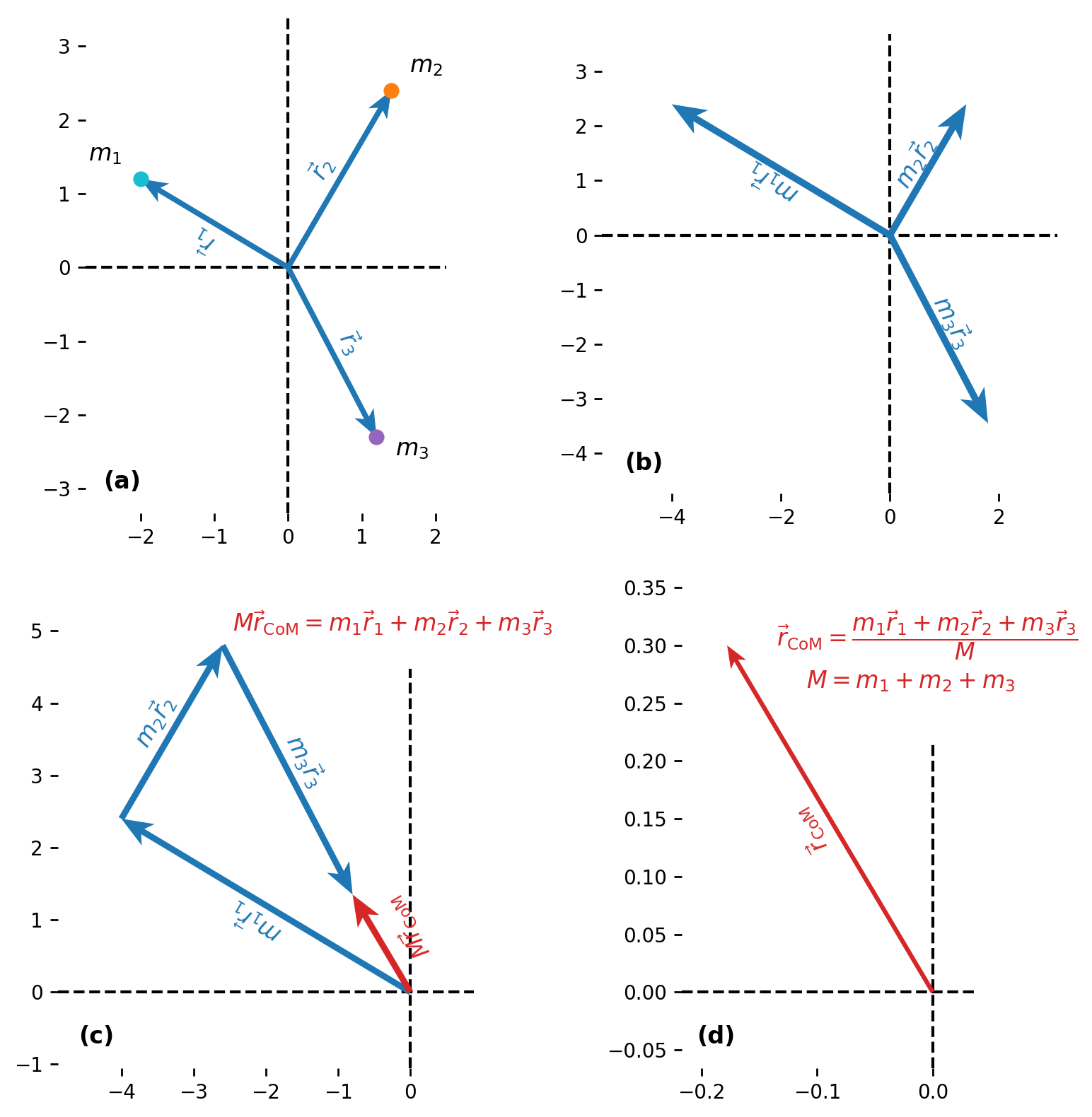
The procedure to find the center-of-mass is illustrated above, where the \(x\) and \(y\) scales show how the position vectors are scaled by the mass.
In general we express a position vector as \(\vec{r}_j = x_j\hat{i} + y_j\hat{j}+z_j\hat{k}\). Then, it follows that:
and thus, we can write the center-of-mass vector \(\vec{r}_{\rm CoM}\) and magnitude \(r_{\rm CoM}\) as:
The same procedure can be applied to the instantaneous velocity, as you might expect, where we have:
which has \(v_x\)-, \(v_y\)-, and \(v_z\)-components.
Problem-Solving Strategy
Calculating the Center-of-Mass
The center-of-mass is a position vector. Follow these steps to calculate it:
Define your coordinate system.
Determine the location of each particle in \(x\), \(y\), and \(z\) coordinates relative to a reference location (usually the origin).
Determine the mass of each particle, and the total (summed) mass (including any mass at the origin).
Calculate the \(r_{\rm CoM,x}\), \(r_{\rm CoM,y}\), and \(r_{\rm CoM,z}\) coordinates. If required, use the Pythagorean theorem to determine its magnitude.
9.6.3.1. Example Problem: Center of Mass of the Earth-Moon System#
Exercise 9.14
The Problem
Using data from the text appendix, determine how far the center of mass of the Earth–Moon system is from the center of Earth. Compare this distance to the radius of Earth, and comment on the result. Ignore all other objects in the solar system.
Show worked solution
The Model
We treat the Earth–Moon system as two point masses separated by the average Earth–Moon distance, and we ignore gravitational interactions with all other bodies. We define the origin of our coordinate system at the center of Earth. Let \(m_E\) and \(m_M\) denote the masses of Earth and Moon, and let \(r_M\) denote the distance from Earth’s center to the Moon. Because the origin is at Earth’s center, \(r_E = 0\). For two objects along a line, the center-of-mass coordinate is \(\displaystyle R = \frac{m_E r_E + m_M r_M}{m_E+m_M}\).
The Math
With \(r_E=0\), the center-of-mass location measured from Earth’s center is
This can be written as a linear combination of the radii \(r_E\) and \(r_M\), where the “coefficients” are mass ratios:
Since \(r_E=0\), the first term drops out, but writing it this way makes the structure of the center-of-mass formula clear.
To show that the answer can be found from ratios alone, we rewrite the remaining coefficient in terms of the single ratio \(m_M/m_E\). Dividing numerator and denominator by \(m_E\) gives
The Moon-to-Earth mass ratio is approximately \(\dfrac{m_M}{m_E} \approx \dfrac{1}{81}\), so
Therefore the center-of-mass distance from Earth’s center is approximately \(R \approx \left(\frac{1}{82}\right) r_M.\)
We now use the observed scale of the Earth–Moon separation relative to Earth’s radius. A commonly used approximate ratio is \(r_M \approx 60\,R_E\) (equivalently \(R_E/r_M \approx 0.017\)). Using this ratio gives
Because \(0.73\,R_E < 1\,R_E\), the Earth–Moon center of mass lies inside Earth.
If we also compute the numerical value using appendix data (\(m_E = 5.97\times 10^{24}\ {\rm kg}\), \(m_M = 7.36\times 10^{22}\ {\rm kg}\), \(r_M = 3.82\times 10^{8}\ {\rm m}\)), we obtain
which matches the ratio-based estimate.
The Conclusion
The center of mass of the Earth–Moon system is at \(R = 4.64 \times 10^{6}\ {\rm m}\) from Earth’s center, which is \(0.73\,R_E\). Since this is less than \(1\,R_E\), the Earth–Moon barycenter lies within Earth.
The key idea is that this conclusion does not require knowing the absolute mass or size of Earth or Moon. It follows from two observable ratios: the mass ratio \(m_M/m_E \approx 1/81\) and the distance ratio \(r_M/R_E \approx 60\). The distance ratio can be determined by angular observations and parallax, and the mass ratio can be inferred from orbital motion, so the essential reasoning is accessible from observation-based astronomy.
The Verification
We verify both approaches in Python by computing \(R\) directly from the appendix values and by computing the dimensionless ratio \(R/R_E\) from the mass ratio and distance ratio. The code mirrors the analytical steps by evaluating the exact center-of-mass expression and the ratio-only estimate.
import numpy as np
m_E = 5.97e24 # mass of Earth (kg)
m_M = 7.36e22 # mass of Moon (kg)
r_M = 3.82e8 # Earth-Moon distance (m)
R_E = 6.37e6 # radius of Earth (m)
R_exact = (m_M*r_M)/(m_E + m_M) # exact center-of-mass distance from Earth's center (m)
ratio_exact = R_exact/R_E # exact center-of-mass distance in Earth radii
mass_ratio = 1/81 # approximate Moon-to-Earth mass ratio
radius_ratio = 60 # approximate Earth-Moon distance in Earth radii
ratio_est = (mass_ratio/(1 + mass_ratio))*radius_ratio # ratio-only estimate for R/R_E
print(f"The exact Earth-Moon center-of-mass distance is {R_exact:.3e} m from Earth's center.")
print(f"The exact value of R/R_E is {ratio_exact:.3f}.")
print(f"The ratio-only estimate gives R/R_E = {ratio_est:.3f}.")
print("Both calculations show that the Earth-Moon barycenter lies inside Earth.")
import numpy as np
# ---------------- appendix-style values ----------------
m_E = 5.97e24 # Earth mass (kg)
m_M = 7.36e22 # Moon mass (kg)
r_M = 3.82e8 # Earth–Moon distance (m)
R_E = 6.37e6 # Earth radius (m)
# ---------------- exact center of mass distance ----------------
R_exact = (m_M * r_M) / (m_E + m_M)
ratio_exact = R_exact / R_E
# ---------------- ratio-only estimate ----------------
mass_ratio = 1/81 # m_M / m_E (approx)
dist_ratio = 60 # r_M / R_E (approx)
coeff = (mass_ratio) / (1 + mass_ratio) # m_M / (m_E + m_M)
ratio_est = coeff * dist_ratio # (R / R_E)
print(f"Exact center-of-mass distance is {R_exact:.3e} m.")
print(f"Exact ratio R/R_E is {ratio_exact:.3f}.")
print(f"Ratio-only estimate gives R/R_E ≈ {ratio_est:.3f}.")
print("Both confirm that R/R_E < 1, so the barycenter lies inside Earth.")
Exact center-of-mass distance is 4.652e+06 m.
Exact ratio R/R_E is 0.730.
Ratio-only estimate gives R/R_E ≈ 0.732.
Both confirm that R/R_E < 1, so the barycenter lies inside Earth.
9.6.3.2. Example Problem: Center of Mass of a Salt Crystal#
Exercise 9.15
The Problem
A single unit cell of sodium chloride (NaCl) forms a cube of edge length \(a = 2.36 \mathring{A}\) (\(1\ \mathring{A} = 10^{-10}\ {\rm m}\)). The unit cell contains four sodium ions and four chloride ions arranged alternately. Determine the location of the center of mass of the unit cell. Specify the result by its coordinates \((r_{{\rm CoM},x}, r_{{\rm CoM},y}, r_{{\rm CoM},z})\).
Show worked solution
The Model
We impose a Cartesian coordinate system on the cube and place the origin at one corner of the unit cell (at a chloride ion). The cube has edge length \(a\), so all ion positions are combinations of \(0\) and \(a\) along the \(x\), \(y\), and \(z\) directions.
There are eight ions total. The center of mass of a system of particles is given by
where \(M\) is the total mass.
Because the crystal structure is symmetric and the ions alternate uniformly throughout the cube, we expect the center of mass to lie at the geometric center of the cube. We verify this directly.
The Math
The ionic masses are \(m_{\rm Cl} = 35.453\,{\rm u} = 5.885 \times 10^{-26}\ {\rm kg}\) and \(m_{\rm Na} = 22.990\,{\rm u} = 3.816 \times 10^{-26}\ {\rm kg}.\)
There are four of each, so the total mass is \(M = 4m_{\rm Cl} + 4m_{\rm Na} = 3.880 \times 10^{-25}\ {\rm kg}.\)
The eight ion positions are all combinations of \((0,a)\) in \(x\), \(y\), and \(z\). By symmetry, exactly half of the total mass lies on the left at \(x_l=0\) and half on the right at \(x_r=a\). Therefore, the \(x\)-coordinate of the center of mass is
Notice that this is the same argument we used to find the center of mass for the Earth-Moon system in the previous example. The same symmetry argument applies in the \(y\)- and \(z\)-directions, giving
Using \(a = 2.36\ \mathring{A} = 2.36 \times 10^{-10}\ {\rm m}\) gives
The Conclusion
The center of mass of the NaCl unit cell lies at
Thus, the center of mass is exactly at the geometric center of the cube, even though the sodium and chloride ions have different masses. The cubic symmetry ensures equal mass distribution about the midpoint in all three directions.
The Verification
We verify this result numerically by explicitly summing \(m_j \vec{r}_j\) for all eight ions and dividing by the total mass. This code directly implements the definition of the center of mass and confirms that symmetry places it at \((a/2, a/2, a/2)\).
import numpy as np
# ---------------- given values ----------------
a = 2.36e-10 # cube edge length (m)
m_Cl = 5.885e-26 # chloride mass (kg)
m_Na = 3.816e-26 # sodium mass (kg)
# ---------------- positions of the 8 ions ----------------
# corners of the cube (alternating Na and Cl)
positions = np.array([
[0,0,0],
[a,0,0],
[0,a,0],
[a,a,0],
[0,0,a],
[a,0,a],
[0,a,a],
[a,a,a]
])
# assign alternating masses
masses = np.array([m_Cl, m_Na, m_Na, m_Cl, m_Na, m_Cl, m_Cl, m_Na])
# ---------------- compute center of mass ----------------
M = np.sum(masses)
r_cm = np.sum(masses[:,None] * positions, axis=0) / M #The [:,None] on masses is to fix dimensions for multiplication
print(f"Center of mass coordinates: {r_cm[0]:.3e}, {r_cm[1]:.3e}, {r_cm[2]:.3e} m")
print("This confirms the center of mass lies at (a/2, a/2, a/2).")
9.6.4. Center of Mass: Continuous Objects#
If the object has its mass uniformly distributed in space, rather as a collection of discrete (equal mass) particles, then \(m_j\rightarrow dm\), and the summation becomes an integral:
Typically, \(r\) is a characteristic dimension of an object (e.g., sphere, rod). To generate an integrand that can actually be calculated, you need to express the mass element \(dm\) as a function of the mass density of the continuous object and the dimension \(r\).
9.6.4.1. Example Problem: CoM of a Uniform Thin Hoop#
Exercise 9.16
The Problem
Find the center-of-mass of a uniform thin hoop (ring) of total mass \(M\) and radius \(r\).
Show worked solution
The Model
The hoop is uniform and thin, so we treat it as a one-dimensional object of radius \(r\) lying in the \(xy\)-plane. By symmetry, we expect the center of mass to lie at the geometric center of the circle. We parameterize the position of each mass element using the polar angle \(\theta\).
The Math
We place the origin at the center of the hoop and compute the center of mass using the definition
Because the hoop is uniform, its linear mass density \(\lambda\) is constant. Since the total length of the hoop is \(2\pi r\), we have \(\lambda = \frac{M}{2\pi r}.\) A point on the hoop has position
A small arc length \(ds\) corresponds to an angle \(d\theta\), so \(ds = r\,d\theta\). The differential mass is therefore
We use the center of mass definition and substitute the \(\vec{r}\) for a hoop, which gives
Then, we substitute for the mass density \(\lambda = \frac{M}{2\pi r}\) and simplify:
This expression can be broken into components as
Then we have over a full revolution, the integrals of the components:
Therefore, the center-of-mass is given by
The Conclusion
The center of mass of a uniform thin hoop lies at the geometric center of the circle: \(\vec r_{\rm CoM} = 0\hat{i} + 0\hat{j} = \vec{0}.\)
Although symmetry strongly suggested this result, the integral confirms that the horizontal and vertical mass contributions cancel exactly over a full \(2\pi\) rotation.
The Verification
We can verify this numerically by approximating the integral as a discrete sum of many equally spaced mass elements around the circle. If the reasoning above is correct, the averaged position should approach zero as the number of sample points increases. The numerical result approaches zero in both directions, confirming the analytical derivation.
import numpy as np
# ---------------- given values ----------------
M = 1.0 # total mass (arbitrary, cancels)
r = 1.0 # radius (arbitrary scale)
N = 100000 # number of discrete mass elements
# ---------------- linear density ----------------
lam = M / (2 * np.pi * r)
# ---------------- angular positions ----------------
theta = np.linspace(0, 2*np.pi, N)
# ---------------- discrete approximation of CM ----------------
x_vals = r * np.cos(theta)
y_vals = r * np.sin(theta)
x_cm = np.mean(x_vals)
y_cm = np.mean(y_vals)
print(f"The numerically determined center of mass x-coordinate: {x_cm:.6e}")
print(f"The numerically determined center of mass y-coordinate: {y_cm:.6e}")
print("As expected, both values are approximately zero.")
9.6.5. Center of Mass: Conservation of Momentum#
Suppose you have \(N\) objects with masses \(m_1,\ m_2,\ \dots,\ m_N\) and initial velocities \(\vec{\rm v}_1,\ \vec{\rm v}_2,\ ldots,\ \vec{\rm v}_N\). The center of mass of the objects is
and its velocity is
Thus, the initial momentum of the center-of-mass is
After these masses move and interact with each other, the momentum of the center of mass is
But conservation of momentum tells us that
This implies that conservation of momentum is expressed in terms of the center of mass of the system. Since \(M\) represents the mass of the entire system of particles, it is necessarily constant. in the absence of an external force, the velocity of the center of mass never changes.
Note
The individual momentum of a single particle is free to move around, accelerate in various directions and with various magnitudes in accordance with the net internal force acting on that object at any time. Such a particle’s momentum will not be constant, but the momentum of the entire extended object will be.
9.7. Rocket Propulsion#
Now we deal with the case where the mass of an object is changing. As a rocket lifts off, it burns fuel gases that cause a change to its velocity (and hence its momentum). The acceleration is in the opposite direction of the velocity of the ejected fuel.
Consider a fully fueled rocket ship in deep space that has a total mass \(m_o\) (mass includes both the ship and the fuel).
At some moment in time, the rocket has a velocity \(\vec{\rm v}\) and mass \(m\) (mass includes the ship and only the remaining fuel).
The rocket accelerates by burning the fuel it carries and ejecting the burned exhaust gases.
If the burn rate of the fuel and the velocity at which the exhaust is ejected is constant, what is the change of velocity of the rocket as a result of burning all of its fuel?
Rockets accelerate by throwing mass backward. As you watch, focus on how the expelled fuel carries momentum in one direction while the rocket gains momentum in the opposite direction. The important point is that a rocket does not need air to push against; it accelerates by exchanging momentum with its own fuel.
9.7.1. Physical Analysis#
Here’s a more detailed description in physical terms:
The rocket engines are continuously ejecting gases, which have some momentum due to their mass and velocity. By conservation of momentum, the rocket’s momentum changes by this same amount (with the opposite sign).
The rate of change of the momentum is constant because the rocket is burning fuel at a constant rate.
From \(\vec{F} = d\vec{p}/dt\), there is a constant force on the rocket.
As time goes on, the mass of the rocket continuously decreases because of the ejecting gases. Even though the force on the rocket is constant, the resulting acceleration is not. It is continuously increasing, \(\vec{a} = \vec{F}/m\).
the total change in the rocket’s velocity will depend on the amount of fuel mass burned and that dependence is not linear.
The problem has the mass and velocity of the rocket changing, along with the total mass of the ejected gases. Let’s define our system to be the rocket + fuel, then this is a closed system (since there are not external forces in deep space). As a result, momentum is conserved for this system (see Fig. 9.4) and we can apply the conservation of momentum to answer the question.
Fig. 9.4 Rocket thrust comes from the momentum carried away by expelled fuel. Image Credit: Openstax: Rocket Propulsion.#
The total instantaneous rocket mass is \(m\) (i.e., the mass of the ship + the amount of fuel at time \(t\)). We define the rocket’s instantaneous velocity as \(\vec{\rm v} = v\hat{i}\), where the velocity is measured relative to an inertial reference system (i.e., some star that is barely moving relative to the Galactic center). Thus the initial momentum of the system is
The rocket’s engines are burning fuel at a constant rate and ejecting exhaust gases in the \(-\hat{i}\) direction. During an infinitesimal time \(dt\), the engines eject a (positive) infinitesimal mass of gas \(dm_g\) at velocity \(\vec{\rm u} = -u\hat{i}\); note that the exhaust gas velocity is measured with respect to the moving rocket. The gas speed measured relative to the star is \((v-u)\hat{i}\).
As a consequence of the ejection of the fuel gas, the rocket’s mass decreases by \(dm_g\) and it velocity increases by \(dv\hat{i}\). We can write the new momentum \(\vec{p}^f\) after this change as
Since all vectors are in the same direction, we drop the vector notation. Applying conservation of momentum, we have
Now, \(dm_g\) and \(dv\) are each very small (infinitesimal even); thus their product very, very small and we neglect this term. This is similar to adding a nanometer to a kilometer; it’s still roughly a kilometer. We obtain:
Since \(dm_g\) represents an increase in the mass of ejected gases, ti must also represent a decrease in the mass of the rocket: \(dm_g = -dm\). Then we have
Integrating from the initial mass \(m_o\) to the final mass \(m\) gives us
This result is called the rocket equation and is typically given as a difference equation
It was originally derived by the Russian rocket scientist Konstantin Tsiolkovsky in 1897. It gives us the change in velocity that the rocket obtains from burning a mass of fuel that decreases the total rocket mass from \(m_o\) to \(m\).
Problem-Solving Strategy
Rocket Propulsion
In rocket problems, the most common questions are finding the \(\Delta v\) due to burning some amount of fuel for some amount of time, or to determine the acceleration \(a\) that results from burning fuel.
To determine the \(\Delta v\), use the rocket equation directly.
To determine the acceleration, determine the force by using the impulse-momentum theorem, where the rocket equation determines the change in velocity.
Checkpoint
For a rocket, why can the force be constant while the acceleration changes with time?
9.7.1.1. Example Problem: Thrust on a Spacecraft#
Exercise 9.17
The Problem
A spacecraft moves in deep space along a straight path. Its thrusters eject fuel at a constant rate of \(200\ {\rm kg/s}\) with an exhaust speed (relative to the rocket) of \(250\ {\rm m/s}\).
The initial mass of the spacecraft (including fuel) is \(2.0 \times 10^4\ {\rm kg}\), and the thrusters fire for \(30\ {\rm s}\).(a) What is the thrust on the spacecraft?
(b) What is the spacecraft’s acceleration as a function of time while the thrusters fire?
(c) What are the accelerations at \(t = 0,\ 15,\ 30,\) and \(35\ {\rm s}\)?
Show worked solution
The Model
We define the system as the spacecraft. The thrust arises from conservation of momentum: fuel is expelled backward, giving the spacecraft forward momentum. Because fuel is ejected at a constant rate and constant exhaust speed, the thrust force is constant. However, the spacecraft’s mass decreases with time as fuel is burned. Therefore, although the force is constant, the acceleration is not constant. We define the forward direction as positive.
The Math
The thrust equals the rate at which momentum is carried away by the exhaust. Since the exhaust speed is constant,
While the engines fire, the spacecraft’s mass decreases linearly:
From Newton’s 2nd law, the acceleration is
Now we, evaluate at the time \(t = 0,\ 15,\ 30,\) and \(35\ {\rm s}\)
After \(t=30\ {\rm s}\), the thrusters are off and \(F=0\), so
The Conclusion
The thrust on the spacecraft is \(F = 5.0 \times 10^4\ {\rm N}\). While the engines fire, the acceleration is given by
The acceleration increases from \(2.5\ {\rm m/s^2}\) at launch to \(3.6\ {\rm m/s^2}\) at \(30\ {\rm s}\) because the mass decreases as fuel is burned. Once the thrusters stop, the acceleration drops to zero and the spacecraft continues at constant velocity.
The Verification
We verify the results numerically by computing the thrust first, then evaluating the time-dependent acceleration using \(a(t)=F/(M-\dot{m}t)\). This mirrors the analytical derivation: constant thrust combined with decreasing mass.
import numpy as np
# ---------------- given values ----------------
M = 2.0e4 # initial mass (kg)
mdot = 2.0e2 # mass ejection rate (kg/s)
v_ex = 2.5e2 # exhaust speed (m/s)
# ---------------- compute thrust ----------------
F = v_ex * mdot
# ---------------- acceleration function ----------------
def a(t):
if t <= 30:
return F / (M - mdot*t)
else:
return 0.0
# ---------------- evaluate specific times ----------------
times = [0, 15, 30, 35]
print(f"Thrust = {F:.2e} N")
for t in times:
print(f"The rocket's acceleration at t = {t} s is {a(t):.3f} m/s^2.")
9.7.2. Rocket in a Gravitational Field#
Let’s analyze the rocket’s velocity change during the launch phase from the surface of the Earth. For simplicity, we consider cases where the acceleration due to gravity is approximately a constant \(g\).
The analysis is similar, except there is an external force \(\vec{F} = -mg\hat{j}\) acting on our system. This force applies an impulse \(d\vec{J} = \vec{F}dt=-mgdt\hat{j}\), which is equal to the change of momentum. This gives us
and so
where we neglect the term \(dm_gdv\) and drop the vector notation. Replacing \(dm_g\) with \(-dm\) gives
Dividing through by \(m\) to solve for \(v\) gives us
and integrating, we have
Unsurprisingly, the rocket’s velocity is affected by the (constant) acceleration of gravity.
The burn time of the fuel is represented by \(\Delta t\). In the absence of gravity, it make no difference how much time it takes to burn the entire mass of fuel because the \(\Delta v\) is independent of \(\Delta t\). The \(-g\Delta t\) term tells us that the longer the burn time is, the smaller the rocket’s change of velocity will be. This is why for a rocket launch it is essential to burn the fuel as quickly as possible to get a large \(\Delta v\).
9.8. In-class Problems#
9.8.1. Part I#
Problem 1
A car of mass \(2000\ {\rm kg}\) is moving with a constant velocity of \(10\ {\rm m/s}\) due east. What is the momentum of the car?
Problem 2
One hazard of space travel is debris left by previous missions. There are several thousand objects orbiting Earth that are large enough to be detected by radar, but there are far greater numbers of very small objects, such as flakes of paint.
Calculate the force exerted by a \(0.100\ \text{mg}\) chip of paint that strikes a spacecraft window at a relative speed of \(4.0 \times 10^3\ {\rm m/s}\) if the collision lasts \(6.0 \times 10^{-8}\ {\rm s}\).
Problem 3
Train cars are coupled together by being bumped into one another. Suppose two loaded train cars are moving toward one another. The first has a mass of \(1.50 \times 10^5\ {\rm kg}\) and a velocity of \((0.30\ {\rm m/s})\hat{i}\), and the second has a mass of \(1.10 \times 10^5\ {\rm kg}\) and a velocity of \(-(0.12\ {\rm m/s})\hat{i}\). What is their final velocity?
Problem 4
A \(20\text{-kg}\) child is coasting at \(3.3\ {\rm m/s}\) over flat ground in a \(4.0\ \text{kg}\) wagon.
a. If the child drops a \(1\ \text{kg}\) ball out the back of the wagon, what is the final speed of the child and wagon?
b. If the child drops a \(1\ \text{kg}\) ball out the back of the wagon so that the ball is at rest relative to the ground, what is the final speed of the child and wagon?
9.8.2. Part II#
Problem 5
In an elastic collision, a \(400\ \text{kg}\) bumper car collides directly from behind with a second, identical bumper car that is traveling in the same direction. The initial speed of the leading bumper car is \(5.6\ {\rm m/s}\) and that of the trailing car is \(6.0\ {\rm m/s}\). Assuming that the mass of the drivers is much, much less than that of the bumper cars, what are their final speeds?
Problem 6
Two particles of masses \(m_1\) and \(m_2\) separated by a horizontal distance \(D\) are released from the same height \(h\) at the same time. Assume no air resistance. Find the (a) vertical position of the center-of-mass of these two particles at a time before the two particles strike the ground, and (b) the distances of the masses relative to the center-of-mass.
Problem 7
Two asteroids collide and stick together. The first asteroid has mass \(1.5 \times 10^4\ {\rm kg}\) and is initially moving at \(770\ {\rm m/s}\). The second asteroid has mass \(2.0 \times 10^4\ {\rm kg}\) and is moving at \(1020\ {\rm m/s}\). Their initial velocities make an angle of \(20^\circ\) with respect to each other. What is the final speed and direction with respect to the velocity of the first asteroid?
Problem 8
A rocket takes off from Earth and reaches a speed of \(100\ {\rm m/s}\) in \(10\ {\rm s}\). If the exhaust speed is \(1500\ {\rm m/s}\) and the mass of fuel burned is \(100\ {\rm kg}\), what was the initial mass of the rocket?
9.9. Homework#
9.9.1. Conceptual Problems#
Problem 1
An object that has a small mass and an object that has a large mass have the same momentum. Which object has the largest kinetic energy?
Problem 2
Can objects in a system have momentum while the momentum of the system is zero? Explain your answer.
9.9.2. Quantitative Problems#
Problem 3
A hockey puck of mass \(150\ {\rm g}\) is sliding due east on a frictionless table with a speed of \(10\ {\rm m/s}\). Suddenly, a constant force of magnitude \(5\ {\rm N}\) directed due north is applied to the puck for \(1.5\ {\rm s}\).
Find the north and east components of the puck’s momentum at the end of the \(1.5\text{-s}\) interval.
Problem 4
A billiard ball, labeled 1, moving horizontally strikes another billiard ball, labeled 2, at rest. Before impact, ball 1 was moving at a speed of \(3.0\ {\rm m/s}\), and after impact it is moving at \(0.5\ {\rm m/s}\) at \(50^\circ\) from the original direction. If the two balls have equal masses of \(300\ {\rm g}\), what is the velocity of ball 2 after the impact?
Problem 5
A \(5.50\ \text{kg}\) bowling ball moving at \(9.0\ {\rm m/s}\) collides with a \(0.85\ \text{kg}\) bowling pin, which is scattered at an angle of \(15.8^\circ\) to the initial direction of the bowling ball and with a speed of \(15.0\ {\rm m/s}\).
a. Calculate the final velocity (magnitude and direction) of the bowling ball.
b. Is the collision elastic?
Problem 6
(a) A \(5.0\ \text{kg}\) squid initially at rest ejects \(0.25\ {\rm kg}\) of fluid with a velocity of \(10\ {\rm m/s}\). What is the recoil velocity of the squid if the ejection is done in \(0.10\ {\rm s}\) and there is a \(5.0\ \text{N}\) frictional force opposing the squid’s movement?
(b) How much energy is lost to work done against friction?