Newton’s Laws of Motion

5. Newton’s Laws of Motion#

May 29, 2026 | 12400 words | 62 min read

Chapter roadmap

This chapter introduces Newton’s laws of motion as the foundation for connecting forces to changes in motion. Forces describe interactions between objects, and Newton’s laws explain how those interactions determine acceleration, equilibrium, and the motion that follows.

As you read, focus on three questions:

What forces act on the object or system?
What direction does each force point?
How does the net force determine the object’s acceleration?

These ideas will be used to build free-body diagrams, connect forces to motion, and prepare for more realistic applications in the next chapter.

5.1. Forces#

The study of motion is called kinematics, which describes the way objects move through their velocity and acceleration.

The study of what causes objects to move is called dynamics, which describes the motion of objects and systems through forces. The foundation of dynamics are the laws of motion developed by Isaac Newton, although some of the fundamental principles were developed earlier by Galileo Galilei.

The development of Newton’s laws marked a transition from Renaissance thinking (i.e., reliance on ancient texts) to Scientific Revolution thinking which developed many of the fundamental pillars of the modern era. Newton’s description of mechanics is now described as classical mechanics where it applies to most situations until the 20th century. The development of modern physics was prompted by discoveries of subatomic particles which move at speeds comparable to the speed of light. To describe the motions of these particles, we need quantum mechanics.

5.1.1. Working Definition of Force#

We need a “working” definition of a force to help build some intuition until we get to the more formal definition given by Newton’s 2nd Law. An intuitive definition of a force is

a push or a pull.

A push or a pull has both magnitude (i.e., how hard) and a direction, so it is a vector quantity. Force can be represented by vectors or expressed as a multiple of a standard force.

Our everyday experience gives a good idea of how multiple forces add. If 2 people push in different directions on a third person (see Fig. 5.1), we might expect the total force to be in the direction of the resultant vector (or force). Forces, like vectors, are represented by arrows.

Checkpoint

A book is sliding across a table and slowing down.

Does the book need a force in the direction of motion to keep moving? Explain briefly.

force as vectors — Fig. 5.1 (a) An overhead view of two ice skaters pushing on a third skater. Forces are vectors and add like other vectors, so the total force on the third skater is in the direction shown. (b) A free-body diagram representing the forces acting on the third skater. Figure Credit: OpenStax: Forces#

Recall the spherical cow, where the solution was for an idealized and simplified situation. Physicists use free-body diagrams (or FBDs) to visualize and simplify our analysis of forces. A FBD is not a lifelike drawing, where it is only a sketch to organize your thinking.

A free-body diagram is not judged for beauty, symmetry, or originality. It is judged only on whether every force acting on the object is there.

The object or system is represented by

a single isolated point (or free body), and
only those forces acting on it (i.e., external forces) are shown.

Drawing Free-Body Diagrams

A free-body diagram is a simple sketch that helps us focus on the forces acting on one object or system. Instead of drawing every detail in the scene, we isolate the object and represent each force with an arrow.

When drawing a free-body diagram:

Choose the object or system you want to analyze.
Represent the object with a simple shape, such as a point or box. This should be in 1980s style graphics as a point, circle, triangle, or rectangle. Place it at the origin of an $xy$-coordinate system.
Draw each force acting on that object as an arrow.
Label each force so its physical source is clear.
Choose coordinate axes that make the problem easier to describe.
Draw a separate free-body diagram for each object in the problem.

The goal is not to make realistic art. The goal is to make the force relationships clear enough that Newton’s laws can be applied.

free-body diagram strategy — Fig. 5.2 In these free-body diagrams, $\vec{N}$ is the normal force, $\vec{w}$ is the weight of the object, and $\vec{f}$ is the friction. Figure Credit: OpenStax: Forces#

The strategy is illustrated in Fig. 5.2 with 2 examples. The video below gives a more in-depth general explanation.

Bozeman Science

This video explains how free-body diagrams can be used to solve kinematics problems.

5.1.2. Contact and Field Forces#

Let’s analyze force more deeply. Suppose a physics student sits at a table (see Fig. 5.3), working diligently on his homework :wink:.

forces on student — Fig. 5.3 (a) The forces acting on the student are due to the chair, the table, the floor, and Earth’s gravitational attraction. (b) In solving a problem involving the student, we may want to consider only the forces acting along the line running through his torso. A free-body diagram for this situation is shown. Figure Credit: OpenStax: Forces#

What external forces act on him? Can we determine the origin of these forces?

Forces are usually grouped into 2 categories: contact and field forces.

Contact forces are due to direct physical contact between objects. The student in Fig. 5.3 experiences contact forces $\vec{C}$ (from the chair), $\vec{F}$ (from the floor), and $\vec{T}$ (from the table).
Field forces act without the necessity of physical contact between objects. They depend on the presence of a “field” near the body under consideration. Earth’s gravitational field causes the student to feel a gravitational force $\vec{w}$, which is his weight.

Checkpoint

Classify each force as a contact force or a field force: gravity, tension, normal force, friction.

Khan Academy

This video explains how forces that act across a distance (e.g., gravity) can be explained using the idea of fields.

As far as we know, there are only 4 fundamental force fields in nature. These are gravitational, electromagnetic, strong nuclear, and weak fields.

The gravitational field is responsible for the weight of a body.
The forces of electricity and magnetism are responsible for the attraction among atoms in bulk matter.
The strong nuclear and weak forces are effective over a short distance, no larger than an atomic nucleus.

Contact forces are fundamentally electromagnetic. Atomic charges interact electromagnetically with other atomic charges, which prevents objects from moving through one another (i.e., no clipping).

5.1.3. Vector Notation for Force#

The SI unit of force is called the Newton (abbreviated $\rm N$), which is the force needed to accelerate an object with a mass of $1\ {\rm kg}$ at a rate of $1\ {\rm m/s^2}$ (i.e., $1\ {\rm N} = 1\ {\rm kg \cdot m/s^2}$). Note that a small apple has a weight of about $1\ \rm N$.

We can describe a force in the form

\[\begin{align*} \vec{F} &= a\hat{i} + b\hat{j}, &\quad \text{(in 2D)} \\ \vec{F} &= a\hat{i} + b\hat{j} + c\hat{k}. &\quad \text{(in 3D)} \end{align*}\]

In Fig. 5.1, let’s suppose that ice skater 1 (on the left) pushes horizontally with a force of $30\ {\rm N}$ to the right (or $\vec{F}_1 = 30 \hat{i}\ {\rm N}$). Similarly, if ice skater 2 (on the bottom) pushes with a force of $40\ {\rm N}$ in the positive vertical direction, we would write $\vec{F}_2 = 40\hat{j}\ {\rm N}$.

The resultant force causes the third ice skater to accelerate. The net external force $\vec{F}_{\rm net}$ is found by taking the vector sum of all external forces acting on an object or system. We can then represent the net external force (in general) as:

(5.1)#\[\begin{align} \vec{F}_{\rm net} &= \sum \vec{F}_{\rm ext}, \\ &= \vec{F}_1 + \vec{F}_2 + \cdots + \vec{F}_N, \\ & = F_{{\rm net},x}\hat{i} + F_{{\rm net},y}\hat{j} + F_{{\rm net},z}\hat{k}, \\ &= \sum_{i=1}^N F_{ix}\hat{i} + \sum_{i=1}^N F_{iy}\hat{j} + \sum_{i=1}^N F_{iz}\hat{k}. \end{align}\]

In this example, we have $\vec{F}_{\rm net} = \vec{F}_1 + \vec{F}_2 = 30\hat{i} + 40\hat{j}\ {\rm N}$. To find the magnitude of the net (resultant) force $F_{\rm net}$, we sum the squares of the components and take the square root, or

\[ F_{\rm net} = \sqrt{(30\ {\rm N})^2 + (40\ {\rm N})^2} = 50\ {\rm N}, \]

where the direction is given by

\[ \theta = \tan^{-1}\! \left(\frac{F_{net,y}}{F_{net,x}}\right) = \tan^{-1}\! \left(\frac{40}{30}\right) = 53^\circ \]

measured from the positive $x$-axis, as shown in the free-body diagram in Fig. 5.1b.

Checkpoint

Two forces act on an object: $\vec{F}_1 = 4\,\hat{i}\ {\rm N}$ and $\vec{F}_2 = -4\,\hat{i}\ {\rm N}$.

What is the net force?

Let’s suppose the ice skaters now push the third ice skater with $\vec{F}_1 = 3\hat{i} + 8\hat{j}\ {\rm N}$ and $\vec{F_2} = 5\hat{i} + 4\hat{j}\ {\rm N}.$

What is the resultant of these two forces?

We recognize that force is a vector, and therefore, we must add using the rules for vector addition:

\[\begin{align*} \vec{F}_{\rm net} &= \sum_{i=1}^2 F_{ix}\hat{i} + \sum_{i=1}^2 F_{iy}\hat{j},\\ &= (3 + 5)\hat{i} + (8 + 4)\hat{j}, \\ &= 8\hat{i} + 12\hat{j}\ {\rm N}. \end{align*}\]

5.2. Newton’s 1st Law#

Newton’s 1st law is a restatement of Galileo’s principle of inertia, which states that an object in motion tends to slow down unless some effort is made to keep it moving. Newton’s 1st law gives a deeper explanation of this observation.

Newton’s 1st Law of Motion

An object at rest remains at rest, and an object in motion remains in motion with constant velocity, unless acted on by a net external force.

Note the expression “constant velocity”, which means that the object maintains a path along a straight line (since neither the magnitude nor direction changes). Also the verb “remains” tells us that it keeps on moving (or not moving) as part of the status quo.

Newton’s 1st law says that there must be a cause for any change in velocity (i.e., acceleration) to occur. The cause is a net external force. An object sliding across a table or floor slows down due to the net force of friction acting on the object. If friction disappears, will the object slow down?

hockey puck on table — Fig. 5.4 An air hockey table is useful in illustrating Newton’s laws. When the air is off, friction quickly slows the puck; but when the air is on, it minimizes contact between the puck and the hockey table, and the puck glides far down the table. Figure Credit: OpenStax: Newton’s First Law#

Consider an air hockey table (Fig. 5.4). When the air is turned off, the puck slides only a short distance before friction slows it to a stop. However, with the air turned on, it creates a nearly frictionless surface, and the puck glides a long distance without slowing down. If we know enough about the friction, we can accurately predict how quickly the object slows down.

Checkpoint

Can an object be moving if the net force on it is zero? Explain using Newton’s first law.

Newton’s 1st law is general and can be applied to anything from an object sliding on table, a satellite in orbit, or even blood pumped from the heart. Experiments have verified that any change in velocity (speed or direction) must be caused by an external force.

Aristotle had claimed that objects had a natural state and needed little “angels” to keep the objects moving. It was Galileo who questioned this idea, which led him to ask the fundamental question: “What is the cause?” Thinking in terms of cause and effect is fundamentally different from the typical ancient Greek approach.

5.2.1. Gravitation and Inertia#

Regardless of the scale of an object, two properties remain valid: gravitation and inertia because they are both connected to mass.

Mass is a measure of the amount of matter in something. It has volume and takes up space.
Gravitation is the attraction of one mass to another. The magnitude of this attraction is your weight, and it is a force.

Mass is related to inertia, which is the ability of an object to resist changes in its motion, or to resist acceleration. Newton’s 1st law is often called the law of inertia.

5.2.2. Inertial Reference Frames#

Newton’s 1st law can also be stated as “Every body remains in its state of uniform motion in a straight line unless it is compelled to change that state by forces acting on it.”

To Newton, “uniform motion in a straight line” meant constant velocity, which includes the special case of zero velocity (or rest).

Therefore the 1st law says that the velocity of an object remains constant if the net force on it is zero, or

\[ \vec{F}_{\rm net} = \sum \vec{F}_{ext} = 0. \]

Newton’s 1st law is also considered as a statement about reference frames. It provides a method for identifying a special type of reference frame called the inertial reference frame.

In principle, we can make the net force on a body zero, if its velocity relative to a given reference frame is constant and then that frame is defined as inertial (recall Section 4.4.3). An inertial reference frame is one where Newton’s 1st law is valid.

Inertial Reference Frame

A reference frame moving at constant velocity relative to an inertial reference frame is also inertial. A reference frame accelerating relative to an inertial frame is not inertial.

Are inertial frames common in nature?

A reference frame at rest to the most distant (or “fixed”) stars is inertial. All frames moving uniformly with respect to this fixed-star frame are also inertial. For example, a nonrotating reference frame attached to the Sun is (for all practical purposes) inertial because its velocity relative to the fixed stars does not vary by more than one part in $10^{10}$.

Earth accelerates relative to the fixed stars because it rotates on its axis and revolves around the Sun. Hence a reference frame attached to its surface is not inertial. For most problems, such a frame serves as a sufficiently accurate approximation to an inertial frame because the acceleration relative to the fixed stars is small (${\sim}10^{-2}\ {\rm m/s^2}$). Thus we consider reference frames fixed to the Earth as inertial.

No particular inertial frame is more special than any other. All inertial frames are equivalent. In analyzing a problem, we choose one particular inertial frame simply based on convenience.

5.2.3. Newton’s 1st Law and Equilibrium#

Newton’s first law tells us about the equilibrium of a system (i.e., $\vec{F}_{\rm net} = 0$). From Fig. 5.1, the forces combine to form a net external force: $\vec{F}_{\rm net} = \vec{F}_1 + \vec{F}_2$. To create equilibrium, we require a balancing force that will produce a net force of zero.

This force must be equal in magnitude, but opposite in direction to $\vec{F}_{\rm net}$ (i.e., $\vec{F}_{\rm bal} = -\vec{F}_{\rm net}$).

For the ice skaters, we found $\vec{F}_{\rm net} = 30\hat{i} + 40\hat{j}\, {\rm N}$, where the balancing force is

\[\begin{align*} \vec{F}_{\rm bal} &= -\vec{F}_{\rm net}, \\ &= -30\hat{i} - 40\hat{j}\, {\rm N}. \end{align*}\]

Newton’s 1st law in vector form is given as

(5.2)#\[\begin{align} \vec{\rm v} = \text{constant, when } \vec{F}_{\rm net} = \vec{0}\ {\rm N}. \end{align}\]

For the net force to equal zero, the velocity vector $\vec{\rm v}$ of the object is a constant.

Derivative of a Constant (Calculus-framing)

From calculus, we have the constant rule which means that for any function $f(x) = c$ (where $c$ is a constant), the derivative $f^\prime(x) = 0$.

What does this mean for an object moving with constant velocity? We have loosely defined a force as a push or pull (or causing an object to accelerate). Recall the definition of acceleration as

\[ \vec{a} = \frac{d\vec{v}(\rm t)}{dt}, \]

which means the acceleration is the slope of the velocity curve. If $\vec{\rm v}(t) = c$, then the slope is equal to zero.

If there is no acceleration, then there is no net force (assuming mass remains constant). This does not mean that no forces act on the object. It means that all external forces acting on the object balance.

Checkpoint

A car moves in a straight line at constant speed.

Is the car in equilibrium? What does that imply about $\sum \vec{F}_{\rm ext}$?

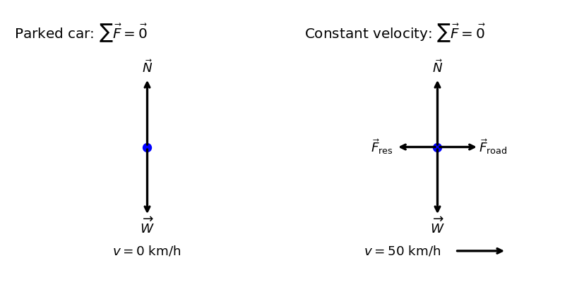
If a car is at rest, the only forces acting on the car are: weight and the contact force pushing up on the car (see Fig. 5.5). A nonzero net force is required to change the state of motion of the car. As a car moves with constant velocity, the friction force propels the car forward and opposes the drag force against it.

net force on car — Fig. 5.5 A car is shown (a) parked and (b) moving at constant velocity. How do Newton’s laws apply to the parked car? What does the knowledge that the car is moving at constant velocity tell us about the net horizontal force on the car? Figure Credit: OpenStax: Newton’s First Law#

Interactive Simulation: Forces and Motion

Use this PhET simulation to explore how an external force will affect the speed and direction of an object's motion. Use free-body diagrams to draw position, velocity, acceleration, and force graphs, and vice versa.

5.2.3.1. Example Problem: Applying Newton’s 1st Law to your car#

Exercise 5.1

The Problem

Newton’s laws can be applied to all physical processes involving force and motion, including something as mundane as driving a car.

(a) Your car is parked outside your house. Does Newton’s first law apply in this situation? Why or why not?

(b) Your car moves at constant velocity down the street. Does Newton’s first law apply in this situation? Why or why not?

The Model

The car is modeled as a single object observed from the ground, which we treat as an inertial reference frame. For the parked car, the coordinate system has $+\hat{j}$ upward. For the moving car, $+\hat{i}$ points in the direction of motion and $+\hat{j}$ points upward. In both cases, the question is not whether forces exist, but whether the vector sum of the external forces is zero.

For the parked car, the only forces that need to be considered are the downward weight and the upward contact force from the ground. For the car moving at constant velocity, the vertical forces still balance, and the horizontal driving force from the road balances the resistive forces from air drag and rolling resistance.

The Math

Newton’s first law applies when the net external force on an object is zero. Under that condition, the acceleration is zero, so the object remains at rest or moves with constant velocity,

\[ \sum \vec{F}_{\rm ext} = \vec{0} \quad \Rightarrow \quad \vec{a}=\vec{0}. \]

For the parked car, the weight acts downward and the ground exerts an upward contact force. Writing these qualitatively as $\vec{W}=-w\,\hat{j}$ and $\vec{N}=n\,\hat{j}$, the force sum is

\[\begin{align*} \sum \vec{F}_{\rm ext} &= \vec{N}+\vec{W},\\ &= n\,\hat{j}-w\,\hat{j},\\ &= (n-w)\,\hat{j}. \end{align*}\]

Since the parked car is not accelerating, the net force is zero and $n=w$. Newton’s first law therefore applies.

For the car moving at constant velocity, the acceleration is still zero. The vertical forces balance as before. In the horizontal direction, the forward force from the road on the tires must balance the backward resistive force. If $\vec{F}_{\rm road}=f\,\hat{i}$ and $\vec{F}_{\rm res}=-f\,\hat{i}$, then

\[ \vec{F}_{\rm road}+\vec{F}_{\rm res}=\vec{0}. \]

The total net force is zero, so Newton’s first law applies in this case as well.

The Conclusion

Newton’s first law applies in both situations. For the parked car, the upward contact force from the ground balances the downward weight. For the car moving at constant velocity, the vertical forces balance and the horizontal driving and resistive forces also balance. The important point is that zero net force means zero acceleration, not necessarily zero velocity.

The Verification

The Python check in the next cell represents each force as a vector and confirms that the net force is zero in both cases. The free-body diagrams are schematic and are used to show balanced forces, not to represent a specific car or numerical force scale.

Show code cell source Hide code cell source

import numpy as np
import matplotlib.pyplot as plt

w = 1.0
n = 1.0
f = 0.6

W_a = np.array([0.0, -w])
N_a = np.array([0.0, +n])
Fnet_a = W_a + N_a

W_b = np.array([0.0, -w])
N_b = np.array([0.0, +n])
F_road = np.array([+f, 0.0])
F_res = np.array([-f, 0.0])
Fnet_b = W_b + N_b + F_road + F_res

print(f"For the parked car, the net force is [{Fnet_a[0]:.1f}, {Fnet_a[1]:.1f}] in arbitrary force units, confirming zero acceleration.")
print(f"For the car moving at constant velocity, the net force is [{Fnet_b[0]:.1f}, {Fnet_b[1]:.1f}] in arbitrary force units, confirming zero acceleration.")
def draw_fbd(ax, forces, labels, note):
    ax.plot(-0.01, 0.0, "bo", markersize=7)
    for F, lab in zip(forces, labels):
        Fx, Fy = F[0], F[1]
        ax.annotate("", xy=(Fx, Fy), xytext=(0.0, 0.0),
                    arrowprops=dict(arrowstyle="->", lw=2))
        # Label placement logic
        if abs(Fx) > abs(Fy):  # horizontal force
            xlab = Fx + 0.2*np.sign(Fx)
            ylab = Fy
            ha, va = "center", "center"
        else:                  # vertical force
            xlab = Fx
            ylab = Fy + 0.15*np.sign(Fy)
            ha, va = "center", "center"
        ax.text(xlab, ylab, lab, fontsize=11, horizontalalignment=ha,verticalalignment=va)

    ax.set_aspect("equal", adjustable="box")
    ax.set_xticks([])
    ax.set_yticks([])
    for spine in ax.spines.values():
        spine.set_visible(False)
    ax.text(0.02, 0.95, note, transform=ax.transAxes, fontsize=12, va="top")
    ax.set_xlim(-2, 2)
    ax.set_ylim(-2, 2)

fig = plt.figure(figsize=(7, 3.8), dpi=120)

ax1 = fig.add_subplot(121)
draw_fbd(ax1, [N_a, W_a],[r"$\vec{N}$", r"$\overrightarrow{W}$"],r"Parked car: $\sum \vec{F}=\vec{0}$")
ax1.text(0.,-1.5,r"$v = 0\ {\rm km/h}$ ",fontsize=11, horizontalalignment='center',verticalalignment='center')

ax2 = fig.add_subplot(122)
draw_fbd(ax2, [N_b, W_b, F_road, F_res],[r"$\vec{N}$", r"$\overrightarrow{W}$",
          r"$\vec{F}_{\rm{road}}$", r"$\vec{F}_{\rm{res}}$"],r"Constant velocity: $\sum \vec{F}=\vec{0}$")
ax2.text(-0.5,-1.5,r"$v = 50\ {\rm km/h}$ ",fontsize=11, horizontalalignment='center',verticalalignment='center')
ax2.annotate("", xy=(1, -1.5), xytext=(0.25, -1.5),
                    arrowprops=dict(arrowstyle="->", lw=2))
plt.tight_layout()
plt.show()

For the parked car, the net force is [0.0, 0.0] in arbitrary force units, confirming zero acceleration.
For the car moving at constant velocity, the net force is [0.0, 0.0] in arbitrary force units, confirming zero acceleration.

../_images/51b0ffe19a1bddbfea63d815aca95d89f21fa9d6204630c3672736dbf91745ed.png

5.3. Newton’s 2nd Law#

Newton’s 2nd law gives the cause-and-effect relationship between force and changes in motion. It is quantitative and used extensively to calculate what happens in situations involving a force.

5.3.1. Force and Acceleration#

What do we mean by a change in motion?

A change in motion is equivalent to a change in velocity (i.e., an acceleration). Newton’s 1st law says that a net external force causes a change in motion, and thus, we see that a net external force causes nonzero acceleration.

An external force is one that is outside the system of interest. In Fig. 5.6a, the system of interest is the car plus the person within it. The two forces exerted by the students outside are external forces.
An internal force acts between elements of the system. Thus the force the person exerts holding onto the steering wheel is an internal force.

external force on car — Fig. 5.6 Figure Credit: OpenStax: Newton’s Second Law#

Only external forces affect the motion of a system, according to Newton’s 1st law. Therefore, we must define the boundaries of the system to separate the internal from external forces.

In Fig. 5.6a, there are arrows denoting the external forces present:

The weight $\vec{w}$ includes the car + person inside.
The car is supported by the ground $\vec{N}$, which will cancel the weight, since the car is not floating nor sinking.
The friction $f$ resists the motion and must be oriented opposite (to the left).
The forces from each student pushing ($\vec{F}_1$ and $\vec{F}_2$) are applied to accelerate the car to the right.

All the forces add together to produce the net force $\vec{F}_{\rm net}$ (see Fig. 5.6b). The free-body diagram (Fig. 5.6a) shows all of the forces acting on the system, where the dot at the center represents the center-of-mass. Forces in the same direction are shown collinearly.

In Fig. 5.6c, a larger net external force produces a larger acceleration $\left(\vec{a}^\prime > \vec{a}\right)$ when the tow truck pulls the car. The acceleration is proportional to and in the same direction as the net external force acting on a system. Mathematically this is written as

\[ \vec{a} \propto \vec{F}_{\rm net}, \]

where the symbol $\propto$ (or \propto) means “proportional to.”

Once the system of interest is chosen, identify the external force and ignore the internal ones. It is a huge simplification to disregard the numerous internal forces acting between objects within the system. This simplification helps us solve some complex problems.

Recall that inertia is the “resistance to motion” and is related to an objects mass. Therefore it seems reasonable that a more massive object requires more acceleration for it to move.

In Fig. 5.7, the same net external force applied to a basketball produces a much smaller acceleration when it is applied to an SUV.

free-body diagrams for force — Fig. 5.7 The same force exerted on systems of different masses produces different accelerations. (a) A basketball player pushes on a basketball to make a pass. (Ignore the effect of gravity on the ball.) (b) The same player exerts an identical force on a stalled SUV and produces far less acceleration. (c) The free-body diagrams are identical, permitting direct comparison of the two situations. Figure Credit: OpenStax: Newton’s Second Law#

Therefore, we can write the proportional relationship between acceleration and mass as

\[ a \propto \frac{1}{m}, \]

where $m$ is the mass of the system and $a$ is the magnitude of the acceleration. Combining the two proportionalities yields Newton’s 2nd law.

Checkpoint

The same net force is applied to two carts. Cart B has twice the mass of cart A.

Which cart has the larger acceleration?

Newton’s 2nd Law of Motion

The acceleration of a system is

directly proportional to the external force acting on the system,
in the same direction as the external force acting on the system, and
inversely proportional to its mass.

In equation form, Newton’s 2nd law is

(5.3)#\[\begin{align} \vec{a} &= \frac{\vec{F}_{\rm net}}{m}, \\ \\ \vec{F}_{\rm net} &= \sum \vec{F} = m\vec{a}. \end{align}\]

Since the mass $m$ is a scalar, we can see that it scales the vector $\vec{a}$ to give the net external force $\vec{F}_{\rm net}$. Also we can use the properties of vectors to write the scalar equivalent as

(5.4)#\[\begin{align} F_{\rm net} = ma. \end{align}\]

5.3.1.1. Example Problem: Pushing a Lawnmower#

Exercise 5.2

The Problem

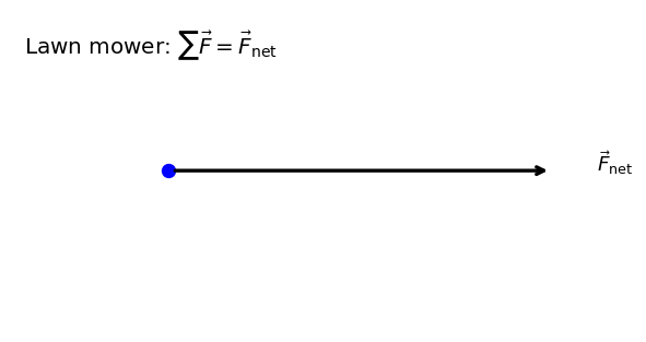
Suppose that the net external force (push minus friction) exerted on a lawn mower is $51\ \text{N}$ (about $11\ \text{lb}.)$ parallel to the ground (Figure 5.8). The mass of the mower is $24\ \text{kg}$. What is its acceleration?

net force on mower — Fig. 5.8 (a) The net force on a lawn mower is 51 N to the right. At what rate does the lawn mower accelerate to the right? (b) The free-body diagram for this problem is shown. Figure Credit: OpenStax: Newton’s Second Law#

The computed acceleration of the lawn mower is 2.1 m/s^2.
Multiplying the mass by this acceleration gives 51 N, which confirms the given net force.

../_images/8d7acf7397901a35339aa59dbff7d61c0a1204890d5d8836a9eec18606ba31c3.png

5.3.1.2. Example Problem: Comparing Forces#

Exercise 5.3

The Problem

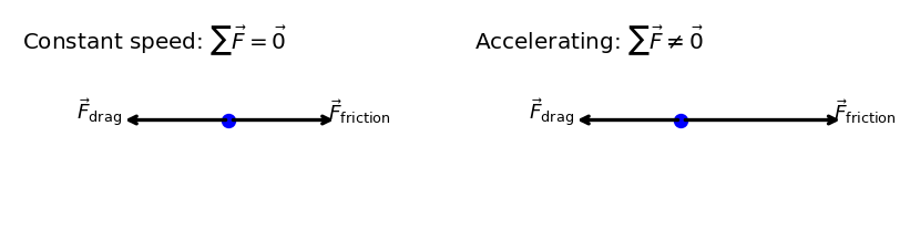
(a) The car shown in Figure 5.9 is moving at a constant speed. Which force is bigger, $\vec{F}_{\text{friction}}$ or $\vec{F}_{\text{drag}}$? Explain.

(b) The same car is now accelerating to the right. Which force is bigger, $\vec{F}_{\text{friction}}$ or $\vec{F}_{\text{drag}}$? Explain.

comparing forces on car — Fig. 5.9 A car is shown (a) moving at constant speed and (b) accelerating. How do the forces acting on the car compare in each case? (a) What does the knowledge that the car is moving at constant velocity tell us about the net horizontal force on the car compared to the friction force? (b) What does the knowledge that the car is accelerating tell us about the horizontal force on the car compared to the friction force? Figure Credit: OpenStax: Newton’s Second Law#

../_images/b9b56c73c391ba6996c3bd807dc8b1642cd4d7cf4254a56de4b9d8697b4f4a88.png

5.3.1.3. Example Problem: Thrust on a Sled#

Exercise 5.4

The Problem

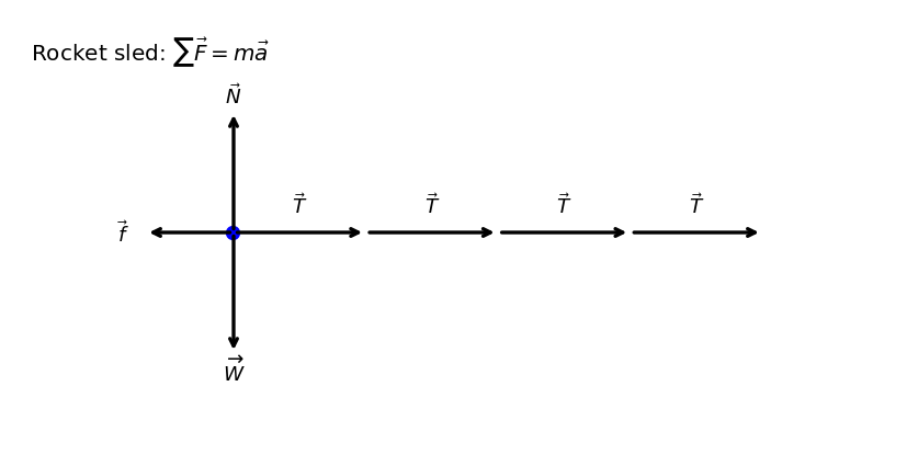
Before space flights carrying astronauts, rocket sleds were used to test aircraft, missile equipment, and physiological effects on human subjects at high speeds. They consisted of a platform that was mounted on one or two rails and propelled by several rockets.

Calculate the magnitude of force exerted by each rocket, called its thrust $T$, for the four-rocket propulsion system shown in Figure 5.10. The sled’s initial acceleration is $49\ \text{m/s}^2$, the mass of the system is $2100\ \text{kg}$, and the force of friction opposing the motion is $650\ \text{N}$.

thrust on a sled — Fig. 5.10 A sled experiences a rocket thrust that accelerates it to the right. Each rocket creates an identical thrust $T$. The system here is the sled, its rockets, and its rider, so none of the forces between these objects are considered. Figure Credit: OpenStax: Newton’s Second Law#

Show code cell source Hide code cell source

import numpy as np
import matplotlib.pyplot as plt

# Given values (2 significant figures)
m = 2100.0      # kg
a = 49.0        # m/s^2
f = 650.0       # N

# Calculations
total_thrust = m*a + f
T = total_thrust/4

# Sig-fig–appropriate output
print(f"The total thrust required from all four rockets is {total_thrust:.1e} N.")
print(f"The thrust required from each rocket is {T:.1e} N.")

# --- Free-body diagram ---
def draw_fbd(ax, forces, labels, note, chain_label=r"$\vec{T}$"):
    ax.plot(-0.01, 0.0, "bo", markersize=7)
    x0, y0 = 0.0, 0.0
    x_chain, y_chain = 0.0, 0.0
    for F, lab in zip(forces, labels):
        Fx, Fy = float(F[0]), float(F[1])
        # Thrusts: draw tip-to-tail (OpenStax style)
        if lab == chain_label:
            ax.annotate("", xy=(x_chain + Fx, y_chain + Fy), xytext=(x_chain, y_chain),
                        arrowprops=dict(arrowstyle="->", lw=2))
            ax.text(x_chain + 0.5*Fx, y_chain + 0.5*Fy + 0.18, lab, fontsize=11,
                    horizontalalignment="center")
            x_chain += Fx
            y_chain += Fy
            continue
        # All other forces: draw from the origin dot
        ax.annotate("", xy=(x0 + Fx, y0 + Fy), xytext=(x0, y0),
                    arrowprops=dict(arrowstyle="->", lw=2))
        # Your label logic (horizontal vs vertical)
        if abs(Fx) > abs(Fy):
            xlab = x0 + Fx + 0.2*np.sign(Fx)
            ylab = y0 + Fy
        else:
            xlab = x0 + Fx
            ylab = y0 + Fy + 0.15*np.sign(Fy)
        ax.text(xlab, ylab, lab, fontsize=11, horizontalalignment="center",verticalalignment="center")
    ax.set_aspect("equal", adjustable="box")
    ax.set_xticks([]) 
    ax.set_yticks([])
    for spine in ax.spines.values(): spine.set_visible(False)
    ax.text(0.02, 0.95, note, transform=ax.transAxes, fontsize=12, va="top")
    ax.set_xlim(-2, 6)
    ax.set_ylim(-2, 2)

# --- Example usage for the rocket sled FBD ---
T_plot = 1.2
f_plot = 0.8
n_plot = 1.1
w_plot = 1.1

forces = [np.array([-f_plot, 0.0]), np.array([0.0, n_plot]), np.array([0.0, -w_plot]),
          np.array([T_plot, 0.0]), np.array([T_plot, 0.0]), np.array([T_plot, 0.0]), np.array([T_plot, 0.0])]

labels = [r"$\vec{f}$", r"$\vec{N}$", r"$\overrightarrow{W}$",
          r"$\vec{T}$", r"$\vec{T}$", r"$\vec{T}$", r"$\vec{T}$"]

fig = plt.figure(figsize=(7, 3.8), dpi=120)
ax = fig.add_subplot(111)
draw_fbd(ax, forces, labels, r"Rocket sled: $\sum \vec{F}=m\vec{a}$")
plt.tight_layout()
plt.show()

The total thrust required from all four rockets is 1.0e+05 N.
The thrust required from each rocket is 2.6e+04 N.

../_images/4b4e9d6f1e5dd1f2a9be2f9066d7e10f1f45dcd7004483431ab129a01bb3ed82.png

5.3.2. Component Form of Newton’s 2nd Law#

Newton’s 2nd law can be written in vector form as

\[ \sum \vec{F}_{\rm ext} = m\vec{a}. \]

Writing this equation in component form gives

(5.5)#\[\begin{align} \sum F_x &= m a_x, \\ \sum F_y &= m a_y, \\ \sum F_z &= m a_z . \end{align}\]

Checkpoint

In the equation $\sum F_x = ma_x$, are $F_x$ and $a_x$ vectors or scalars?

Once we write Newton’s 2nd law in component form, the quantities $F_x$, $F_y$, $F_z$, $a_x$, $a_y$, and $a_z$ are scalars, so vector notation is no longer used. Each component equation relates forces and acceleration along a single axis and can be analyzed independently.

The second law is a description of how a body responds mechanically to its environment. The influence of the environment is the net force $\vec{F}_{\rm net}$, the body’s response is the acceleration $\vec{a}$, and the strength of the response is inversely proportional to the mass $m$. The larger the mass of an object, the smaller its acceleration to a given net force.

Khan Academy

This video reviews how to resolve angled forces into components and apply Newton’s second law along each coordinate axis.

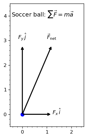
5.3.2.1. Example Problem: Force on a Soccer Ball#

Exercise 5.5

The Problem

A $0.400\ \text{kg}$ soccer ball is kicked across the field by a player; it undergoes acceleration given by $\vec{a} = 3.00\hat{i} + 7.00\hat{j}\ \text{m/s}^2.$ Find (a) the resultant force acting on the ball and (b) the magnitude and direction of the resultant force.

The x-component of the net force is 1.20 N.
The y-component of the net force is 2.80 N.
The magnitude of the net force is 3.05 N.
The direction of the net force is 66.8 degrees above the positive x-axis.

../_images/d0ade75fbc43ed46821056409c0b92a7eb26bca85388fd322007ddc7557862d4.png

5.3.2.2. Example Problem: Mass of a Car#

Exercise 5.6

The Problem

Find the mass of a car if a net force of $-600.0\,\hat{j}\ \text{N}$ produces an acceleration of $-0.2\,\hat{j}\ \text{m/s}^2$.

5.3.2.3. Example Problem: Several Forces#

Exercise 5.7

The Problem

A particle of mass $m = 4.0\ \text{kg}$ is acted upon by four forces of magnitudes $F_1 = 10.0\ \text{N}$, $F_2 = 40.0\ \text{N}$, $F_3 = 5.0\ \text{N}$, and $F_4 = 2.0\ \text{N}$, with the directions as shown in the free-body diagram in Fig. 5.11. What is the acceleration of the particle?

four forces — Fig. 5.11 Four forces in the xy-plane are applied to a 4.0-kg particle. Figure Credit: OpenStax: Newton’s Second Law#

import numpy as np
import matplotlib.pyplot as plt

# -----------------------------
# Given values
# -----------------------------
m = 4.0
F1 = 10.0
F2 = 40.0
F3 = 5.0
F4 = 2.0
theta = np.deg2rad(30.0)

# -----------------------------
# Force components
# -----------------------------
F1_vec = np.array([F1*np.cos(theta), F1*np.sin(theta)])
F2_vec = np.array([0.0, -F2])
F3_vec = np.array([-F3, 0.0])
F4_vec = np.array([0.0, F4])

# Net force and acceleration
F_net = F1_vec + F2_vec + F3_vec + F4_vec
a_vec = F_net / m

# Sig-fig–appropriate output (2 sig figs)
print(f"The net force is ({F_net[0]:.2g} i-hat {F_net[1]:+.2g} j-hat) N.")
print(f"The acceleration is ({a_vec[0]:.2g} i-hat {a_vec[1]:+.2g} j-hat) m/s^2.")

The net force is (3.7 i-hat -33 j-hat) N.
The acceleration is (0.92 i-hat -8.2 j-hat) m/s^2.

5.3.3. Newton’s 2nd Law and Momentum#

Newton actually stated his 2nd law in terms of momentum

“The instantaneous rate at which a body’s momentum changes is equal to the net force acting on the body.”

This is written by the vector equation:

(5.6)#\[\begin{align} \vec{F}_{\rm net} = \frac{d\vec{p}}{dt}. \end{align}\]

Momentum was described by Newton as “quantity of motion,” or a way of combining both the velocity and mass of an object. For now, it’s sufficient to define momentum $\vec{p}$ as the product of the mass of the object $m$ and its velocity $\vec{\rm v}$:

\[ \vec{p} = m\vec{\rm v}. \]

Since velocity is a vector, so is momentum. If we substitute our definition of momentum into Newton’s 2nd law, we find

\[\begin{align*} \vec{F}_{\rm net} &= \frac{d\vec{p}}{dt} = \frac{d(m\vec{\rm v})}{dt}, \\ &= m\frac{d{\vec{\rm v}}}{dt} = m\vec{a}. \end{align*}\]

Thus, we see that the momentum form of Newton’s 2nd law reduces to the form given earlier.

Interactive Simulation: Projectile Motion Models

Use this PHET simulation to explore the forces at work when pulling a cart or pushing a refrigerator, crate, or person. Put an object on a ramp and see how it affects its motion.

5.4. Mass and Weight#

Mass and weight are often used interchangeably in everyday conversation. In physics, however, there is an important distinction. Weight is the pull of gravitational force on an object, where it depends on the distance to the center of an object.

Checkpoint

A $70\ {\rm kg}$ astronaut is far from any planet or star.

What is her mass? What is her weight, approximately?

Unlike weight, mass does not vary with distance. The mass of an object is the same on Earth’s surface, in orbit, or on the surface of the Moon.

Veritasium

This video illustrates the difference between mass and weight through man-on-the-street type interviews.

5.4.1. Units of Force#

The scalar equation $F_{\rm net} = ma$ is used to define the net force in terms of mass, length, and time. The SI unit of force is the newton. Using $F_{\rm net} = ma$, we can see that

\[ 1\ {\rm N} = 1\ {\rm kg \cdot m/s^2}. \]

You’re probably more familiar with another unit of force, which is the pound $(\rm lb)$, where $1\ {\rm lb} = 4.448\ {\rm N}$. An even more historical measurement of weight is the stone, where $1\ {\rm st} = 14\ {\rm lb} \approx 62.3\ {\rm N}$.

Use the Python code below to convert your weight into newtons or stones.

import numpy as np 
lb_to_N = 4.448 # Newtons in a pound
st_to_N = 14*lb_to_N #Newtons in a stone

my_weight = 150 #lbs
weight_N = my_weight*lb_to_N 
weight_st = weight_N/st_to_N
print(f"My weight is {weight_N:.0f} N or about {weight_st:.2g} stone.")

My weight is 667 N or about 11 stone.

5.4.2. Weight and Gravitational Force#

When an object is dropped on Earth, it accelerates toward Earth’s center. Newton’s 2nd law says that a net force on an object is responsible for its acceleration. If air resistance is negligible, the net force on a falling object is the gravitational force, which is called its weight $\vec{w}$, or its force due to gravity acting on an object of mass $m$.

Weight is denoted as a vector because it has a direction (down) and hence, weight is a downward force. The magnitude of weight is denoted by $w$. Using Newton’s 2nd law, we can derive an equation for weight.

Consider an object with mass $m$ falling toward Earth. It experiences only the downward force of gravity, which is the weight $\vec{w}$. Newton’s 2nd law says that the magnitude of the net external force on an object is $\vec{F}_{\rm net} = m\vec{a}$. We know that the acceleration due to gravity is $\vec{g}$, or $\vec{a} = \vec{g}$.

Weight

The gravitational force on an object near Earth is called its weight. Weight is a vector because it has both magnitude and direction. Near Earth’s surface, the weight of an object of mass $m$ is

\[\begin{align*} \vec{w} &= m\vec{g}. \end{align*}\]

If upward is chosen as the positive $y$ direction, then $\vec{g} = -g\,\hat{j}$ and

\[\begin{align*} \vec{w} &= -mg\,\hat{j}. \end{align*}\]

The magnitude of the weight is $w = mg.$

The weight of a $1$-kg object on Earth is $9.81\ {\rm N}$:

\[ w = mg = (1.0\ {\rm kg})(9.81\ {\rm m/s^2}) = 9.81\ {\rm N}. \]

When the net external force on an object is its weight, we say that it is in free fall, which means that the only force acting on the object is gravity.

Acceleration due to gravity $g$ varies slightly over Earth’s surface, so the weight of an object depends on its location and is not an intrinsic property of the object. Weight varies dramatically if we leave Earth’s surface, where on the Moon $g\approx 1.62\ {\rm m/s^2}$ (about 1/6 of the value on Earth’s surface). A $1$-kg weight has a weight of $9.8\ {\rm N}$ on Earth, while it is only $1.6\ {\rm N}$ on the Moon.

Note

Weight and mass are different physical quantities, although they are closely related.

Mass is an intrinsic property of an object: it is a quantity of matter. In most situations, mass does not vary; therefore its response to an applied force does not vary.
Weight is the gravitational force acting on an object, so it does vary depending on gravity. A person at a lower elevation in New Orleans (i.e., closer to Earth’s center) weighs more than someone at high elevation like on top of Mt. Everest (i.e., farther from Earth’s center) even though they have the same mass.

Checkpoint

A $1.0\ {\rm kg}$ object weighs about $9.81\ {\rm N}$ on Earth.

Would the same object have the same mass on the Moon? Would it have the same weight?

Why does it feel comfortable to equate mass and weight?

On Earth, we see that weight $\vec{w}$ is directly proportional to mass $m$, since $\vec{w} = m\vec{g}$. When two quantities are proportional, we develop heuristics to communicate more effectively among people with a shared sense of the heuristic.

Suppose you are asked how far is Dallas, TX from Commerce, TX. You might reply that it is about $1$-hr, depending on traffic. This makes sense because you and your interlocutor both share in the assumption that you will travel by car at about $60\ {\rm mph}$. It is important to note that time is not equal to distance, where you are communicating $x = vt$, where $x$ is proportional to $t$ because of the implicit assumption that $v$ is a constant.

The Earth rotates once every $24$-hr, which means that is about $15^\circ$ per hour. Astronomers developed a measure of distance on the sky called right ascension based on the seemingly constant rotation speed. As a result, it carries units in hours, minute, seconds.

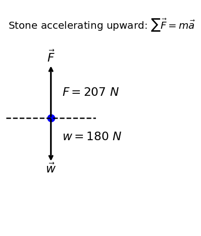
5.4.2.1. Example Problem: Lifting a Stone#

Exercise 5.8

The Problem

A farmer is lifting some moderately heavy rocks from a field to plant crops. He lifts a stone that weighs $40.0\ \text{lb}$ (about $180\ \text{N}$). What force does he apply if the stone accelerates upward at a rate of $1.5\ \text{m/s}^2$?

The computed mass of the stone is 18 kg.
The required upward force applied by the farmer is 210 N.

../_images/4c0ca40728466e785d24625a143dd3d7515fea9eab793f601777a538de284710.png

CrashCourse

This video reviews Newton’s three laws of motion, emphasizing net force and free-body diagrams. Use it as a conceptual refresher before beginning Newton’s third law examples.

5.5. Newton’s 3rd Law#

Newton’s 3rd Law of Motion

For every interaction between two objects, the forces come in pairs. If object $A$ exerts a force on object $B$, then object $B$ exerts a force on object $A$ with equal magnitude and opposite direction.

Using $\vec{F}_{AB}$ to mean “the force on $B$ by $A$” and $\vec{F}_{BA}$ to mean “the force on $A$ by $B$,” Newton’s third law is

\[\begin{align*} \vec{F}_{AB} &= -\vec{F}_{BA}. \end{align*}\]

These two forces act on different objects, so they do not cancel in a free-body diagram of a single object.

Newton’s 3rd law represents a certain symmetry in nature: Forces always occur in pairs, and one body cannot exert a force on another without experiencing a force itself. We sometimes refer to this law loosely as “action-reaction”.

Consider a swimmer pushing off the side of a pool (see Fig. 5.12). She pushes against the pool wall with her feet and accelerates in the opposite direction of her push. The wall has exerted an equal and opposite force on the swimmer.

swim reaction force — Fig. 5.12 When the swimmer exerts a force on the wall, she accelerates in the opposite direction; in other words, the net external force on her is in the direction opposite of $F_{\rm feet\ on\ wall}$. This opposition occurs because, in accordance with Newton’s third law, the wall exerts a force $F_{\rm wall\ on\ feet}$ on the swimmer that is equal in magnitude but in the direction opposite to the one she exerts on it. The line around the swimmer indicates the system of interest. Thus, the free-body diagram shows only $F_{\rm wall\ on\ feet}$, $\vec{w}$ (the gravitational force), and $\overrightarrow{BF}$, which is the buoyant force of the water supporting the swimmer’s weight. The vertical forces $\vec{w}$ and $\overrightarrow{BF}$ cancel because there is no vertical acceleration. Figure Credit: OpenStax: Newton’s Third Law#

You might think that two equal and opposite forces would cancel, but they do not because they act on different systems. In this case, there are two systems that we could investigate: (a) the swimmer and (b) the wall.

(a) If we select the swimmer, then $\vec{F}_\text{wall on feet}$ is an external force on this system and affects the swimmer’s motion. The swimmer moves in the direction of this force.$F_{\rm feet\ on\ wall}$
(b) The force $\vec{F}_\text{feet on wall}$ acts on the wall and thus, it does not directly affect the motion of the swimmer and does not cancel $\vec{F}_\text{wall on feet}$.

The swimmer pushes in the direction opposite that in which she wishes to move. The reaction to her push is thus in the desired direction. In a free-body diagram, we never include both forces of an action-reaction pair, we only use $\vec{F}_\text{wall on feet}$, not $\vec{F}_\text{feet on wall}$.

Other examples of Newton’s 3rd law are easy to find:

A car accelerates forward because the ground pushes forward on the drive wheels, in reaction to the drive wheels pushing backward on the ground.
Rockets move forward by expelling gas backward at high velocity. This reaction force is called thrust, which pushes a body forward in response to a backward force.
Helicopters create lift by pushing air down, thereby experiencing an upward reaction force.

There are two important features of Newton’s 3rd law.

The forces exerted (action and reaction) are always equal in magnitude but opposite in direction.
These forces are acting on different bodies or systems: $A$’s force acts on $B$ and $B$’s force on A. They don’t act on the same body and thus, they do not cancel each other.

Checkpoint

A swimmer pushes backward on a wall.

What is the Newton’s third-law partner to this force, and which object does it act on?

A person who is walking or running applies Newton’s 3rd law instinctively. For example, a runner pushes backward on the ground so that it pushes him forward (see Fig. 5.13).

runner reaction force — Fig. 5.13 The runner experiences Newton’s third law. (a) A force is exerted by the runner on the ground. (b) The reaction force of the ground on the runner pushes him forward. Figure Credit: OpenStax: Newton’s Third Law#

5.5.1. Example Problem: Forces on a Stationary Object#

Exercise 5.9

The Problem

The package in Figure 5.14 is sitting on a scale. For the scale and package at rest (i.e., not accelerating), show that the scale indicates the weight of the package.

scale reaction force — Fig. 5.14 (a) The forces on a package sitting on a scale, along with their reaction forces. The force $\vec{w}$ is the weight of the package (the force due to Earth’s gravity) and $\vec{s}$ is the force of the scale on the package. (b) Isolation of the package-scale system and the package-Earth system makes the action and reaction pairs clear. Figure Credit: OpenStax: Newton’s Third Law#

5.5.2. Example Problem: Force on the Cart (Part 1)#

Exercise 5.10

The Problem

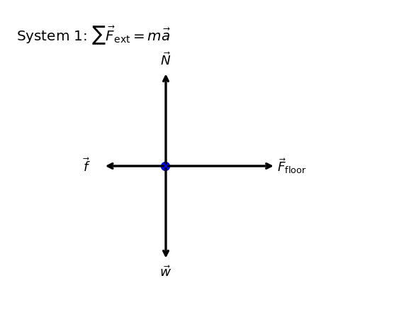
A physics professor pushes a cart of demonstration equipment to a lecture hall (Figure 5.15). Her mass is $65\ {\rm kg}$, the cart’s mass is $12\ {\rm kg}$, and the equipment’s mass is $7\ {\rm kg}$. Calculate the acceleration produced when the professor exerts a backward force of $150\ {\rm N}$ on the floor. All forces opposing the motion, such as friction on the cart’s wheels and air resistance, total $24.0\ {\rm N}$.

cart reaction force — Fig. 5.15 A professor pushes the cart with her demonstration equipment. The lengths of the arrows are proportional to the magnitudes of the forces (except for $\vec{f}$, because it is too small to be drawn to scale). System 1 is appropriate for this example, because it asks for the acceleration of the entire group of objects. Only $\vec{F}_{\rm floor}$ and $\vec{f}$ are external forces acting on System 1 along the line of motion. All other forces either cancel or act on the outside world. System 2 is chosen for the next example so that $\vec{F}_{\rm prof}$ is an external force and enters into Newton’s second law. The free-body diagrams, which serve as the basis for Newton’s second law, vary with the system chosen. Figure Credit: OpenStax: Newton’s Third Law#

Show code cell source Hide code cell source

import numpy as np
import matplotlib.pyplot as plt

# Given values
m_prof = 65.0   # kg
m_cart = 12.0   # kg
m_eq = 7.0      # kg
F_floor = 150.0 # N
f = 24.0        # N

m = m_prof + m_cart + m_eq
F_net = F_floor - f
a = F_net / m

print(f"The total mass of System 1 is {m:.2g} kg.")
print(f"The horizontal net external force on System 1 is {F_net:.3g} N.")
print(f"The acceleration of System 1 is {a:.2g} m/s^2.")

def draw_fbd(ax, forces, labels, note, chain_label=r"$\vec{T}$"):
    ax.plot(-0.01, 0.0, "bo", markersize=7)
    x0, y0 = 0.0, 0.0
    x_chain, y_chain = 0.0, 0.0
    for F, lab in zip(forces, labels):
        Fx, Fy = float(F[0]), float(F[1])
        if lab == chain_label:
            ax.annotate("", xy=(x_chain + Fx, y_chain + Fy), xytext=(x_chain, y_chain),arrowprops=dict(arrowstyle="->", lw=2))
            ax.text(x_chain + 0.5*Fx, y_chain + 0.5*Fy + 0.18, lab, fontsize=11,horizontalalignment="center")
            x_chain += Fx
            y_chain += Fy
            continue
        ax.annotate("", xy=(x0 + Fx, y0 + Fy), xytext=(x0, y0),arrowprops=dict(arrowstyle="->", lw=2))
        if abs(Fx) > abs(Fy):
            xlab = x0 + Fx + 0.2*np.sign(Fx)
            ylab = y0 + Fy
        else:
            xlab = x0 + Fx
            ylab = y0 + Fy + 0.15*np.sign(Fy)
        ax.text(xlab, ylab, lab, fontsize=11, horizontalalignment="center",
                verticalalignment="center")
    ax.set_aspect("equal", adjustable="box")
    ax.set_xticks([])
    ax.set_yticks([])
    for spine in ax.spines.values():
        spine.set_visible(False)
    ax.text(0.02, 0.95, note, transform=ax.transAxes, fontsize=12, va="top")
    ax.set_xlim(-2.0, 2.8)
    ax.set_ylim(-2.0, 2.0)

# FBD (System 1): include all forces shown in the diagram
F_floor_plot = 1.4
f_plot = 0.8
N_plot = 1.2
w_plot = 1.2

forces = [
    np.array([+F_floor_plot, 0.0]),
    np.array([-f_plot, 0.0]),
    np.array([0.0, +N_plot]),
    np.array([0.0, -w_plot]),
]
labels = [
    r"$\vec{F}_{\rm floor}$",
    r"$\vec{f}$",
    r"$\vec{N}$",
    r"$\vec{w}$",
]

fig = plt.figure(figsize=(5,4), dpi=120)
ax = fig.add_subplot(111)
draw_fbd(ax, forces, labels, r"System 1: $\sum \vec{F}_{\rm ext}=m\vec{a}$")
plt.tight_layout()
plt.show()

The total mass of System 1 is 84 kg.
The horizontal net external force on System 1 is 126 N.
The acceleration of System 1 is 1.5 m/s^2.

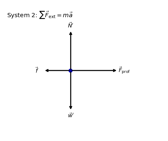
../_images/45d23d414af0f459b259b686dd98e373f70644e9489734bbdf9b93eb0b7efe93.png

5.5.3. Example Problem: Force on the Cart (Part 2)#

Exercise 5.11

The Problem

Calculate the force the professor exerts on the cart in Figure 5.15, using data from the previous example if needed.

Show code cell source Hide code cell source

import numpy as np
import matplotlib.pyplot as plt

# Given values (from the previous example, as needed)
m_cart = 12.0     # kg
m_eq = 7.0        # kg
a = 1.5           # m/s^2
f = 24.0          # N

m = m_cart + m_eq
F_net = m*a
F_prof = F_net + f

print(f"The mass of System 2 is {m:.3g} kg.")
print(f"The net force required to accelerate System 2 is {F_net:.2g} N.")
print(f"The professor's force on the cart is {F_prof:.2g} N.")

def draw_fbd(ax, forces, labels, note, chain_label=r"$\vec{T}$"):
    ax.plot(-0.01, 0.0, "bo", markersize=7)
    x0, y0 = 0.0, 0.0
    x_chain, y_chain = 0.0, 0.0

    for F, lab in zip(forces, labels):
        Fx, Fy = float(F[0]), float(F[1])
        if lab == chain_label:
            ax.annotate("", xy=(x_chain + Fx, y_chain + Fy), xytext=(x_chain, y_chain), arrowprops=dict(arrowstyle="->", lw=2))
            ax.text(x_chain + 0.5*Fx, y_chain + 0.5*Fy + 0.18, lab, fontsize=11, horizontalalignment="center")
            x_chain += Fx
            y_chain += Fy
            continue
        ax.annotate("", xy=(x0 + Fx, y0 + Fy), xytext=(x0, y0), arrowprops=dict(arrowstyle="->", lw=2))
        if abs(Fx) > abs(Fy):
            xlab = x0 + Fx + 0.2*np.sign(Fx)
            ylab = y0 + Fy
        else:
            xlab = x0 + Fx
            ylab = y0 + Fy + 0.15*np.sign(Fy)
        ax.text(xlab, ylab, lab, fontsize=11, horizontalalignment="center",verticalalignment="center")
    ax.set_aspect("equal", adjustable="box")
    ax.set_xticks([])
    ax.set_yticks([])
    for spine in ax.spines.values():
        spine.set_visible(False)
    ax.text(0.02, 0.95, note, transform=ax.transAxes, fontsize=12, va="top")
    ax.set_xlim(-2.0, 2.8)
    ax.set_ylim(-2.0, 2.0)

# --- Free-body diagram (System 2): include all forces shown for the system ---
F_prof_plot = 1.4
f_plot = 0.8
N_plot = 1.2
w_plot = 1.2

forces = [np.array([+F_prof_plot, 0.0]),np.array([-f_plot, 0.0]),np.array([0.0, +N_plot]),np.array([0.0, -w_plot])]
labels = [r"$\vec{F}_{\rm prof}$",r"$\vec{f}$",r"$\vec{N}'$",r"$\vec{w}'$"]

fig = plt.figure(figsize=(5,4), dpi=120)
ax = fig.add_subplot(111)
draw_fbd(ax, forces, labels, r"System 2: $\sum \vec{F}_{\rm ext}=m\vec{a}$")
plt.tight_layout()
plt.show()

The mass of System 2 is 19 kg.
The net force required to accelerate System 2 is 28 N.
The professor's force on the cart is 52 N.

../_images/84dd9b8b4b28d36ca744dd4b3feed4930ef60b0eae409cd3dff8eff9fab074d8.png

Check Your Understanding

Two blocks are at rest and in contact on a frictionless surface. The masses are $m_1 = 2\ {\rm kg}$ and $m_2 = 6\ {\rm kg}$, and an applied force of $24\ {\rm N}$ pushes the blocks together.

(a) Find the acceleration of the system of blocks.

(b) Suppose that the blocks are later separated. What force would give the second block, with mass $6\ {\rm kg}$, the same acceleration as the system of blocks?

5.6. Common Forces#

5.6.1. Normal Force#

Weight is a pervasive force that acts at all times and must be counteracted to keep an object from falling (i.e., in static equilibrium). You must support the weight of a heavy object by pushing up on it when you hold it stationary.

When a bag of dog food is placed on the table (see Fig. 5.16), the table sags slightly under the load. This is more noticeable on a card table, compared to a sturdy oak table. Unless an object is deformed beyond its limit, it will exert a restoring force like a spring. The greater the deformation, the greater the restoring force. The next external force on the load is zero, when the load is stationary on the table.

normal force example — Fig. 5.16 (a) The person holding the bag of dog food must supply an upward force $\vec{F}_{\rm hand}$ equal in magnitude and opposite in direction to the weight of the food $\vec{w}$ so that it doesn’t drop to the ground. (b) The card table sags when the dog food is placed on it, much like a stiff trampoline. Elastic restoring forces in the table grow as it sags until they supply a force $\vec{N} equal in magnitude and opposite in direction to the weight of the load. Figure Credit: OpenStax: Common Forces#

Whatever supports a load must supply an upward force equal to the weight of the load. If the force supporting the weight of an object is perpendicular to the surface of contact, this is defined as a normal force $\vec{N}$. This means that the normal force experienced by an object resting on a horizontal forced can be expressed in vector form and scalar form as:

(5.7)#\[\begin{align} \vec{N} &= m\vec{g}, \\ N &= mg. \end{align}\]

Note

Do not confuse the symbol $N$ for the normal-force magnitude with the unit newton, ${\rm N}$. The normal force is not automatically equal to the object’s weight. It equals whatever value is required by the force balance perpendicular to the surface. For an object at rest on an incline, the normal force balances only the perpendicular component of the weight.

When an object rests on an incline that makes an angle $\theta$ with the horizontal, the force of gravity acting on the object is divided into two components:

a force acting perpendicular to the plane, $w_y$, and
a force acting parallel to the plane, $w_x$.

The normal force $\vec{N}$ is typically equal in magnitude and opposite in direction to $w_y$, where the component parallel to the plane $w_x$ causes the object to accelerate down the incline (see Fig. 5.17). The $w_x$ is the unbalanced force which allows the acceleration to occur, where $w_y$ is balanced by the normal force $N$.

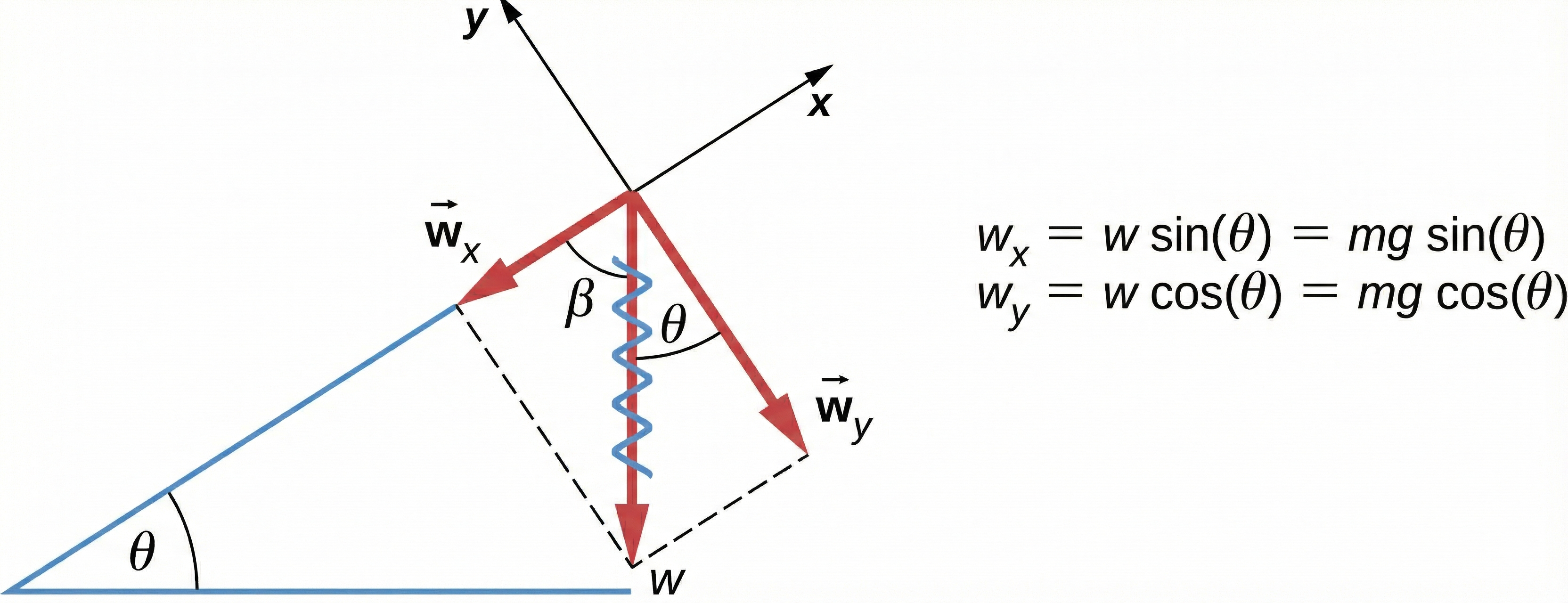
force on an incline example — Fig. 5.17 The coordinate system is chosen so that the $x$-axis is parallel to the inclined surface. The angle $\beta (= 90^\circ - \theta)$ is complementary to $\theta$. Modified from OpenStax Figure 5.23.#

Angles on a Triangle

How do we know that the angle $\theta$ given in Fig. 5.17 is the same in both places?

Let’s assume that they are different:

$\theta_1$ is the angle between between $\vec{w}$ and $\vec{w}_y$,
$\theta_2$ is the angle between the horizontal surface and incline plane.

The angle between $\vec{w}$ and $\vec{w}_x$ is $\beta = 90^\circ - \theta_1$ because $\vec{w}_x$ and $\vec{w}_y$ are perpendicular. The inclined surface also makes a triangle, with 3 angles that sum to $180^\circ$, or

\[ \theta_2 + 90^\circ + \beta = 180^\circ.\]

We can solve for $\beta$ in terms of $\theta_2$ and substitute into the equation for the equation with $\theta_1$,

\[\begin{align*} \beta &= 90^\circ - \theta_2, \\ 90^\circ - \theta_2 &= 90^\circ - \theta_1,\\ \theta_2 &= \theta_1. \end{align*}\]

With a little geometry, we showed that $\theta_1 = \theta_2 = \theta$.

Be careful when resolving the weight into components. Normally when the $x$-component of a force $\vec{F}$ is resolved, we find that $F_x = F\cos{\theta}$. However, in this case we are using the complementary angle $\beta = 90^\circ - \theta$ to resolve the $w_x$. Using the red vectors in Fig. 5.17, we have

\[\begin{align*} w_x &= w\cos{\beta} = w\sin{\theta}, \\ w_y &= w\cos{\theta}. \end{align*}\]

Checkpoint

An object rests on an incline.

Is the normal force usually equal to the object’s full weight $w$, or only to one component of the weight?

We can sum the forces along the $y$-axis to write the magnitude of the normal force experienced by an object resting on an inclined plane:

\[\begin{align*} \sum F_y &= N - mg\cos{\theta} = 0, \\ N &= mg\cos{\theta}. \end{align*}\]

Notice that the force components and normal force could be determined from a free-body diagram.

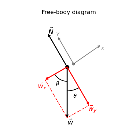
../_images/c4699a47aab715cd60198581d1e2293d665505375f739f1e54536ad6164de3d5.png — Fig. 5.18 Free-body diagram showing $\vec{w}$ resolved into $\vec{w}_x$ and $\vec{w}_y$ in axes aligned with the incline.#

Show code cell content Hide code cell content

import numpy as np
import matplotlib.pyplot as plt
from matplotlib.patches import Arc
from myst_nb import glue
# -----------------------------
# Parameters
# -----------------------------
theta = np.deg2rad(30.0)   # incline angle
w = 1.6                    # weight magnitude (plot units)
N = 1.4*np.cos(theta)                    # normal force magnitude (plot units)
# Weight components in rotated frame
w_x = w * np.sin(theta)
w_y = w * np.cos(theta)

# -----------------------------
# Helper: angle arc marker
# -----------------------------
def draw_angle_arc(ax, v1, v2, radius=0.6, label=r"$\theta$", label_r=0.75, lw=1.5):
    """
    Draw the smaller CCW arc from v1 to v2 (both are 2D direction vectors).
    Places a label near the middle of the arc.
    """
    def ang_deg(v):
        return (np.degrees(np.arctan2(v[1], v[0])) + 360.0) % 360.0
    a1 = ang_deg(v1)
    a2 = ang_deg(v2)
    # CCW sweep from a1 to a2
    delta = (a2 - a1) % 360.0
    if delta > 180.0:
        # Use the smaller arc by swapping
        a1, a2 = a2, a1
        delta = (a2 - a1) % 360.0
    a2_plot = a1 + delta  # ensure CCW arc length = delta
    arc = Arc((0.0, 0.0), 2*radius, 2*radius, angle=0.0, theta1=a1, theta2=a2_plot, lw=lw)
    ax.add_patch(arc)
    amid = np.radians(a1 + 0.5*delta)
    ax.text(label_r*np.cos(amid), label_r*np.sin(amid), label, fontsize=11,
            ha="center", va="center")
# -----------------------------
# Free-body diagram function
# -----------------------------
def draw_fbd(ax, forces, labels, note, colors=None):
    ax.plot(0, 0, "k.", markersize=15)
    if colors is None:
        colors = ["black"]*len(forces)
    for F, lab, col in zip(forces, labels,colors):
        Fx, Fy = F
        ax.annotate("",xy=(Fx, Fy),xytext=(0, 0),
            arrowprops=dict(arrowstyle="->", lw=2,color=col, shrinkA=0, shrinkB=0))
        # Label placement
        if abs(Fx) > abs(Fy):
            ax.text(Fx * 1.05-0.2, Fy-0.2, lab, color=col, ha="left", va="center", fontsize=14)
        else:
            ax.text(Fx+0.1, Fy * 1.08-0.025, lab, color=col, ha="center", va="center", fontsize=14)
    ax.set_aspect("equal", adjustable="box")
    ax.set_xticks([])
    ax.set_yticks([])
    for spine in ax.spines.values():
        spine.set_visible(False)
    ax.text(0.3, 0.95, note, transform=ax.transAxes, fontsize=12, va="top")

# -----------------------------
# Coordinate axes (rotated)
# -----------------------------
x_hat = np.array([np.cos(theta), np.sin(theta)])
y_hat = np.array([-np.sin(theta), np.cos(theta)])
# Directions for components (down-slope and into the plane-normal direction)
wx_dir = -x_hat
wy_dir = -y_hat
w_dir  = np.array([0.0, -1.0])  # weight direction (down)
# -----------------------------
# Forces
# -----------------------------
forces = [
    np.array([0.0, -w]),                        # weight
    np.array([N * y_hat[0], N * y_hat[1]]),     # normal force (along +y_hat)
    np.array([w_x * wx_dir[0], w_x * wx_dir[1]]),  # w_x (along -x_hat)
    np.array([w_y * wy_dir[0], w_y * wy_dir[1]])   # w_y (along -y_hat)
]
labels = [r"$\vec{w}$",r"$\vec{N}$",r"$\vec{w}_x$",r"$\vec{w}_y$"]
colors = ["k","k","r","r"]

# -----------------------------
# Plot
# -----------------------------
fig = plt.figure(figsize=(6, 4), dpi=120)
ax = fig.add_subplot(111)

draw_fbd(ax, forces, labels, r"Free-body diagram",colors=colors)
# --- Parallelogram construction (dashed lines) ---
w_tip  = forces[0]
wx_tip = forces[2]
wy_tip = forces[3]
ax.plot([wx_tip[0], w_tip[0]],[wx_tip[1], w_tip[1]],
        linestyle="--", linewidth=1.2, color="red")
ax.plot([wy_tip[0], w_tip[0]],[wy_tip[1], w_tip[1]],
        linestyle="--", linewidth=1.2, color="red")

# Draw coordinate axes
x_offset, y_offset = 0.2,0.1
ax.annotate("", xy=(x_hat[0]+x_offset, x_hat[1]+0.2), xytext=(x_offset, y_offset),
            arrowprops=dict(arrowstyle="->", lw=1.5,alpha=0.5))
ax.text(1.1*x_hat[0]+0.1, 1.1*x_hat[1], r"$x$", fontsize=11,alpha=0.5)

ax.annotate("", xy=(y_hat[0]+x_offset, y_hat[1]+0.1), xytext=(x_offset, y_offset),
            arrowprops=dict(arrowstyle="->", lw=1.5,alpha=0.5))
ax.text(1.1*y_hat[0]+x_offset, 1.1*y_hat[1]+y_offset/2, r"$y$", fontsize=11,alpha=0.5)
ax.plot(x_offset,0.1,'.',color='gray',ms=10)

# -----------------------------
# Angle markers
#   theta: between w and w_y direction (-y_hat)
#   beta : between w and w_x direction (-x_hat)
# -----------------------------
draw_angle_arc(ax, w_dir, wy_dir, radius=0.75, label=r"$\theta$", label_r=0.95)
draw_angle_arc(ax, wx_dir, w_dir, radius=0.45, label=r"$\beta$", label_r=0.60)

ax.set_xlim(-2., 2.)
ax.set_ylim(-2., 2.)

plt.tight_layout()
glue("fbd_weight_components", fig, display=False)
fig.savefig("inclined_FBD.png",bbox_inches='tight',dpi=150);
plt.show();

5.6.1.1. Example Problem: Weight on an incline#

Exercise 5.12

The Problem

Consider the skier on the slope in Figure 5.19. Her mass including equipment is $60.0\ \text{kg}$. (a) What is her acceleration if friction is negligible? (b) What is her acceleration if friction is $45.0\ \text{N}$?

skier incline example — Fig. 5.19 Since the acceleration is parallel to the slope and acting down the slope, it is most convenient to project all forces onto a coordinate system where one axis is parallel to the slope and the other is perpendicular to it (axes shown to the left of the skier). $\vec{N}$ is perpendicular to the slope and $\vec{f}$ is parallel to the slope, but $\vec{w}$ has components along both axes, namely, $w_y$ and $w_x$. Here, $\vec{w}$ has a squiggly line to show that it has been replaced by these components. The force $\vec{N}$ is equal in magnitude to $w_y$, so there is no acceleration perpendicular to the slope, but $f$ is less than $w_x$, so there is a downslope acceleration (along the axis parallel to the slope). Figure Credit: OpenStax: Common Forces#

Show code cell source Hide code cell source

import numpy as np
import matplotlib.pyplot as plt
from matplotlib.patches import Arc

# Given values
m = 60.0            # kg
g = 9.81            # m/s^2
theta = np.deg2rad(25.0)
f = 45.0            # N

# Weight components
w = m * g
w_x = w * np.sin(theta)
w_y = w * np.cos(theta)
# Accelerations
a_no_fric = w_x / m
a_with_fric = (w_x - f) / m
print(f"The skier's acceleration without friction is {a_no_fric:.1f} m/s^2 down the slope.")
print(f"The skier's acceleration with friction is {a_with_fric:.1f} m/s^2 down the slope.")

# Normal force (just balanced visually)
N = w_y
# frictional force (just to make better visually on FBD)
f *= 3 #this is equivalent to f = 3*f
# -----------------------------
# Helper: angle arc marker
# -----------------------------
def draw_angle_arc(ax, v1, v2, radius=0.6, label=r"$\theta$", label_r=0.75, lw=1.5):
    def ang_deg(v):
        return (np.degrees(np.arctan2(v[1], v[0])) + 360.0) % 360.0
    a1 = ang_deg(v1)
    a2 = ang_deg(v2)
    delta = (a2 - a1) % 360.0
    if delta > 180.0:
        a1, a2 = a2, a1
        delta = (a2 - a1) % 360.0
    arc = Arc((0, 0), 2*radius, 2*radius,
              theta1=a1, theta2=a1+delta, lw=lw)
    ax.add_patch(arc)
    amid = np.radians(a1 + delta/2)
    ax.text(label_r*np.cos(amid), label_r*np.sin(amid),
            label, ha="center", va="center", fontsize=11)
# -----------------------------
# Free-body diagram function
# -----------------------------
def draw_fbd(ax, forces, labels, note, colors=None):
    ax.plot(0, 0, "k.", ms=15)
    if colors is None:
        colors = ["black"] * len(forces)
    for F, lab, col in zip(forces, labels, colors):
        ax.annotate("", xy=F, xytext=(0, 0),
            arrowprops=dict(arrowstyle="->", lw=2,color=col, shrinkA=0, shrinkB=0))
        Fx, Fy = F
        if abs(Fx) > abs(Fy):
            ax.text(1.08*Fx-0.05, Fy+0.1, lab, color=col,
                    ha="center", va="center", fontsize=13)
        else:
            ax.text(Fx, 1.08*Fy-0.025, lab, color=col,
                    ha="center", va="center", fontsize=13)
    ax.set_aspect("equal")
    ax.set_xticks([])
    ax.set_yticks([])
    for spine in ax.spines.values():
        spine.set_visible(False)
    ax.text(0.05, 0.95, note, transform=ax.transAxes,
            fontsize=12, va="top")
# -----------------------------
# Rotated coordinate axes
# -----------------------------
x_hat = np.array([np.cos(theta), np.sin(theta)])
y_hat = np.array([-np.sin(theta), np.cos(theta)])
wx_dir = -x_hat
wy_dir = -y_hat
w_dir  = np.array([0.0, -1.0])
# -----------------------------
# Forces
# -----------------------------
plot_scale = 1 / w   # normalize weight to length 1
forces = [
    np.array([0.0, -w]),                  # weight
    N * y_hat,                             # normal
    w_x * wx_dir,                          # w_x
    w_y * wy_dir,                          # w_y
    f * x_hat                              # friction (upslope)
]
forces = plot_scale*np.array(forces)

labels = [r"$\vec{w}$",r"$\vec{N}$",r"$\vec{w}_x$",r"$\vec{w}_y$",r"$\vec{f}$"]
colors = ["k", "k", "r", "r", "b"]

# -----------------------------
# Plot
# -----------------------------
fig = plt.figure(figsize=(6, 4), dpi=120)
ax = fig.add_subplot(111)

draw_fbd(ax, forces, labels, "Free-body diagram", colors)

# Parallelogram construction
w_tip  = forces[0]
wx_tip = forces[2]
wy_tip = forces[3]

ax.plot([wx_tip[0], w_tip[0]],[wx_tip[1], w_tip[1]], "r--", lw=1.2)
ax.plot([wy_tip[0], w_tip[0]],[wy_tip[1], w_tip[1]], "r--", lw=1.2)

# Draw coordinate axes
x_offset, y_offset = 0.5,0.2
ax.annotate("", xy=(0.5*x_hat[0]+x_offset, 0.5*x_hat[1]+y_offset), xytext=(x_offset, y_offset),
            arrowprops=dict(arrowstyle="->", lw=1.5,alpha=0.5))
ax.text(0.6*x_hat[0]+0.4, 0.6*x_hat[1]+y_offset/2, r"$x$", fontsize=11,alpha=0.5)

ax.annotate("", xy=(0.5*y_hat[0]+x_offset, 0.5*y_hat[1]+y_offset), xytext=(x_offset, y_offset),
            arrowprops=dict(arrowstyle="->", lw=1.5,alpha=0.5))
ax.text(0.6*y_hat[0]+x_offset, 0.6*y_hat[1]+y_offset/2, r"$y$", fontsize=11,alpha=0.5)
ax.plot(x_offset,0.2,'.',color='gray',ms=10)

# Angle markers
draw_angle_arc(ax, w_dir, wy_dir, radius=0.4, label_r=0.55,label=r"$25\degree$")
draw_angle_arc(ax, wx_dir, w_dir, radius=0.25, label_r=0.35,label=r"$65\degree$")

# -----------------------------
# Proper scaling
# -----------------------------
L = max(np.linalg.norm(F) for F in forces)
ax.set_xlim(-1.4*L, 1.4*L)
ax.set_ylim(-1.4*L, 1.4*L)

plt.tight_layout()
plt.show()

The skier's acceleration without friction is 4.1 m/s^2 down the slope.
The skier's acceleration with friction is 3.4 m/s^2 down the slope.

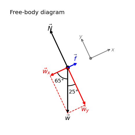
../_images/308edbc51e68d186c8a803d9882ee88b083d6de51f5a4e571990db399c814de1.png

5.6.2. Tension#

A tension is a force along the length of a medium, such as a rope or cable. The word “tension” comes from a Latin word meaning “to stretch”. Any flexible connecter (e.g., string, rope, wire, or cable) can exert a pull parallel to its length. Consider the phrase: “You can’t push a rope.” Instead tension force pulls outward along the two ends of a rope.

tension example — Fig. 5.20 When a perfectly flexible connector (one requiring no force to bend it) such as this rope transmits a force $\vec{T}$, that force must be parallel to the length of the rope, as shown. By Newton’s third law, the rope pulls with equal force but in opposite directions on the hand and the supported mass (neglecting the weight of the rope). The rope is the medium that carries the equal and opposite forces between the two objects. The tension anywhere in the rope between the hand and the mass is equal. Once you have determined the tension in one location, you have determined the tension at all locations along the rope. Figure Credit: OpenStax: Common Forces#

Consider a person holding a $5.0$-kg mass on a rope (see Fig. 5.20). If the mass is stationary, then its acceleration is zero and the net force is zero. The only external forces acting on the mass are its weight $w$ and the tension $T$ supplied by the rope. Thus,

\[ \vec{F}_{\rm net} = T-w = 0, \]

where the $+\hat{j}$ direction defines up. The tension equals the weight of the supported mass,

\[ T = w = mg, \]

hanging at rest. For a $5.0$-kg mass (neglecting the mass of the rope), we see that

\[ T = mg = \left(5.0\ {\rm kg}\right)\left(9.81\ {\rm m/s^2}\right) = 49\ {\rm N}. \]

If we cut the rope and insert a spring, the spring would extend a length corresponding to a force of $49\ {\rm N}$, providing a direct observation and measure of the tension force in the rope.

Checkpoint

If a light rope is cut and a spring scale is inserted, what force does the scale measure?

Does it measure the sum of the pulls from both sides, or the tension in the rope?

tension tightrope example — Fig. 5.21 The weight of a tightrope walker causes a wire to sag by $5.0^\circ$. The system of interest is the point in the wire at which the tightrope walker is standing. Figure Credit: OpenStax: Common Forces#

Large Tension

If we wish to create a large tension, we need to exert a force perpendicular to a taut flexible connector (see Fig. 5.21). The weight of the tightrope walker acts as a force perpendicular to the rope.

Suppose that the tightrope walker is standing still, so the net force in both directions zero. We can decompose the tension into 2 components: right $\vec{T}_R$ and left $\vec{T}_L$.

Each section of rope is supporting the weight $\vec{w}$ through their $y$ components: $T_{Ly}$ and $T_{Ry}$.
The $x$ component of the weight is balanced through each section of the rope, where $T_{Lx} = T_{Rx}$.

The net force is given as

\[\begin{align*} F_{{\rm net},y} &= T_{Ry} + T_{Ly} - w = 0, \\ F_{{\rm net},x} &= T_{Rx} - T_{Lx} = 0, \end{align*} \]

where we treat the tightrope walker as a particle at the center of the vectors, the $+\hat{i}$ direction goes to the right of the walker, and up is in the $+\hat{j}$ direction above the walker.

We can examine the $x$-components first, where the rope bends from the horizontal by an angle $\theta$ so that

\[\begin{align*} T_{Rx} &= T_R\cos{\theta}, \\ T_{Lx} &= T_L\cos{\theta}, \\ T_R\cos{\theta} &= T_L\cos{\theta}. \end{align*}\]

Since $\cos{\theta} \neq 0$, this implies $T_R = T_L$.

From the example with the hanging mass (Fig. 5.20), we saw that the tension acts along the rope and is the same magnitude everywhere. If we cut the rope then the same tension $T$ acts along both strands, not the sum of the forces from both sides. As a result we can treat the left and right sides of the rope as having the same tension $T$, or

\[ \boxed{T_R = T_L = T.}\]

Turning to the $y$-components, we have $T_{Ry}$ and $T_{Ly}$ both in the positive direction and $T_{Ry} = T_{Ly} = T\sin{\theta}$ using the same logic from the $x$-component analysis. Therefore, we can write the $y$-components as

\[\begin{align*} 2T\sin{\theta} - w &= 0, \\ 2T\sin{\theta} &= w, \\ T &= \frac{w}{2\sin{\theta}}. \end{align*}\]

Since the weight $w = mg$, we have

\[ \boxed{T = \frac{mg}{2\sin{\theta}}.}\]

We can extend this expression to describe the tension $T$ when a perpendicular force ($F_{\perp}$, or F_{\perp}) is exerted at the middle of a flexible connector:

\[ T = \frac{F_\perp}{2\sin{\theta}}. \]

In this case, $T$ becomes large as $\theta \to 0$. Even the relatively small weight of any flexible connector will cause it to sag, since an infinite tension would result if it were horizontal (i.e., $\sin{\theta}=0$).

5.6.2.1. Example Problem: Tension in a Tightrope#

Exercise 5.13

The Problem

Calculate the tension in the wire supporting the $70.0\ \mathrm{kg}$ tightrope walker shown in Figure 5.21.

tension tightrope FBD example — Fig. 5.22 When the vectors are projected onto vertical and horizontal axes, their components along these axes must add to zero, since the tightrope walker is stationary. The small angle results in $T$ being much greater than $w$. Figure Credit: OpenStax: Common Forces#

5.6.3. Friction#

Friction is a resistive force the opposes motion. The normal force acts in the opposite direction as the weight to keep an object at rest on a horizontal surface.

Checkpoint

A block remains at rest on a rough incline.

What force prevents the block from sliding down the incline?

If the surface is tilted, the normal force balances the component of the weight perpendicular to the surface (i.e., $N = w_y$).
If the object does not slide downward, the friction balances the component of the weight parallel to the inclined plane (i.e., $f = w_x$).

5.6.4. Spring Force#

A spring is a special medium that has the ability to restore its shape. To restore its shape, a spring exerts a restoring force that is proportional to and in the opposite direction in which it is stretched or compressed.

The spring force is also known as Hooke’s law, which has a mathematical form

(5.8)#\[\begin{align} \vec{F} = -k\vec{x}, \end{align}\]

where $\vec{x}$ measures the position relative to the rest (relaxed) position $x_o = 0$ and the constant $k$ measures the spring’s stiffness (an intrinsic property).

The line of action is parallel to the spring axis, which means we can use the scalar form:

(5.9)#\[\begin{align} F = -k(x-x_o), \end{align}\]

where $x$ is measured along the spring axis. We can now see that the restoring force is:

positive when the spring is compressed; $x-x_o<0$,
negative when the spring is stretched; $x-x_o>0$.

spring forceexample — Fig. 5.23 A spring exerts its force proportional to a displacement, whether it is compressed or stretched. Image Credit: OpenStax: Common Forces#

Interactive Simulation: Hooke’s Law

Use this PhET simulation to explore the relationships among force, spring constant, and displacement. Investigate what happens when two springs are connected in series and in parallel.

5.6.5. Real Forces and Inertial Frames#

Some forces are real, whereas others are not. Real forces have some physical origin, such as gravity, tension, or friction. Fictitious forces appear only because the observer is using an accelerating or rotating frame of reference.

For example, consider a satellite moving due north above Earth’s Northern Hemisphere. To an observer on Earth, the satellite appears to be pushed westward. However, there is no physical force acting on the satellite in that direction. Instead Earth is rotating eastward beneath it. The apparent westward force exists only because Earth’s frame of reference is rotating.

Real forces always come in action-reaction pairs. If no physical object experiences the reaction force, then the force is fictitious.

5.7. Drawing Free-body Diagrams#

The first step in describing and analyzing most phenomena in physics involves the careful drawing of a free-body diagram (FBD). FBDs have been used throughout this chapter. A FBD must only include the external forces acting on the body of interest.

Once we have drawn an accurate FBD, we can apply

Newton’s 1st law if the body is in equilibrium ($F_{\rm net} = 0$), or
Newton’s 2nd law if the body is accelerating ($F_{\rm net} \neq 0$).

Checkpoint

Should the net force be drawn as a separate arrow on a free-body diagram? Explain why or why not.

MIT OpenCourseWare

This worked example shows how to draw separate free-body diagrams for interacting blocks and apply Newton’s second law to each system.

Constructing Free-Body Diagrams

Observe the following rules when constructing a FBD:

Draw the object under consideration as a simpler shape (e.g., point, box, etc.). It does not have to be artistic. We often place the object at the origin of an $xy$-coordinate system.
Include all forces that act on the object, representing these forces as vectors. Do not include the net force on the object. We never include both forces of an action-reaction pair.
Convert the FBD into a more detailed diagram showing the $x$- and $y$-components of a given force. In this case place a squiggly line through the original vector to show that it is no longer in play (i.e., replaced by components).
If there are more than a single object in the problem, draw a separate FBD for each object.

If there is acceleration, we do not directly include it in the FBD. However, it may help to indicate acceleration outside the FBD.

Khan Academy

This video shows how to identify all forces acting on an object, represent them with a free-body diagram, and resolve angled forces into horizontal and vertical components to determine the net force and resulting motion.

Let’s apply the problem-solving strategy in drawing a FBD for a sled. In Fig. 5.24a, a sled is pulled by force $\vec{P}$ at a $30^\circ$ angle.

In part (b), we show a free-body diagram as described by steps 1 and 2.
In part (c), we show all forces in terms of their $x$- and $y$-components, in keeping with step 3.

skier tension example — Fig. 5.24 (a) A moving sled is shown as (b) a free-body diagram and (c) a free-body diagram with force components. Figure Credit: OpenStax: Drawing Free-body Diagrams#

5.7.1. Example Problem: Two Blocks on an Inclined Plane#

Exercise 5.14

The Problem

Construct the free-body diagram for object A and object B in Figure 5.25.

2 blocks FBD example — Fig. 5.25 (a) The free-body diagram for isolated object A. (b) The free-body diagram for isolated object B. Comparing the two drawings, we see that friction acts in the opposite direction in the two figures. Friction always acts opposite the direction of motion or intended motion. Because object A is moving to the right, friction by B must act to the left. Object B is moving to the left relative to B, so the friction by A on B is to the right. The friction force by object A on object B is the third law pair of the friction force by B on A, and therefore these two forces must be in opposite directions. Because object B is sliding down the incline, the friction force by the ramp must oppose it and act up the ramp. Figure Credit: OpenStax: Drawing Free-body Diagrams#

Show code cell source Hide code cell source

import numpy as np
import matplotlib.pyplot as plt

# -----------------------------
# Incline geometry
# -----------------------------
theta = np.deg2rad(30.0)

# Unit vectors parallel and perpendicular to incline
x_hat = np.array([np.cos(theta), np.sin(theta)])
y_hat = np.array([-np.sin(theta), np.cos(theta)])

# -----------------------------
# draw_fbd helper
# -----------------------------
def draw_fbd(ax, forces, labels, note, colors=None,offsets=None,label_offsets=None):
    ax.plot(0, 0, "b.", markersize=15)
    if colors is None:
        colors = ["black"] * len(forces)
    if offsets is None:
        offsets = [np.array([0.0, 0.0])] * len(forces)
    if label_offsets is None:
        label_offsets = [(6, 6)] * len(forces)  # default like your current
    # --- draw arrows + labels (labels use offset points so they don't rescale axes) ---
    for F, lab, col, off, laboff in zip(forces, labels, colors, offsets,label_offsets):
        Fx, Fy = F
        ox, oy = off
        ax.annotate("", xy=(Fx + ox, Fy + oy), xytext=(ox, oy),arrowprops=dict(arrowstyle="->",
                    lw=2, color=col, shrinkA=0, shrinkB=0))
        dx_pts, dy_pts = laboff
        ax.annotate(lab, xy=(Fx + ox, Fy + oy), xytext=(dx_pts, dy_pts), textcoords="offset points",
            color=col, fontsize=14, ha="center", va="bottom")
    # --- scaling: set limits from max vector length ---
    mags = [np.hypot(F[0], F[1]) for F in forces]
    R = 1.25 * max(mags + [1e-6])  # padding; avoid zero
    ax.set_xlim(-R, R)
    ax.set_ylim(-R, R)
    ax.set_aspect("equal", adjustable="box")
    ax.set_xticks([])
    ax.set_yticks([])
    for spine in ax.spines.values():
        spine.set_visible(False)
    ax.text(0.03, 0.95, note, transform=ax.transAxes, fontsize=12, va="top")
    ax.plot([-1*x_hat[0], 0], [-x_hat[1], 0],linestyle="--",color="gray",lw=1.2)
    ax.text(-0.9*x_hat[0], -1.1*x_hat[1], r"$-x$", color="gray", fontsize=11)
# -----------------------------
# Object A forces
# -----------------------------
wA = np.array([0.0, -1.0])
T  = 0.8 * x_hat
N_BA = 0.7 * y_hat
f_BA = -0.4 * x_hat
forces_A = [wA, T, N_BA, f_BA]
labels_A = [r"$\vec{w}_A$", r"$\vec{T}$", r"$\vec{N}_{BA}$", r"$\vec{f}_{BA}$"]
# Label offsets for A (tweak as you like)
label_offsets_A = [
    (0, -20),   # w_A a bit below its tip
    (0, 6),    # T slightly to the right
    (-4, 4),   # N_BA slightly left/up
    (-6, 6),  # f_BA down/left so it doesn't sit on dashed -x
]
# -----------------------------
# Object B forces
# -----------------------------
wB = np.array([0.0, -1.2])
N_B = 1.3 * y_hat
f_B = 0.5 * x_hat
N_AB = -N_BA
f_AB = -f_BA
forces_B = [wB, N_B, f_B, N_AB, f_AB]
labels_B = [r"$\vec{w}_B$",r"$\vec{N}_B$",r"$\vec{f}_B$",r"$\vec{N}_{AB}$",r"$\vec{f}_{AB}$"]

#Use offsets when two vectors point in the same direction
d = 0.12  # tweak 0.08–0.18 depending on your plotting scale
offsets = [np.array([0.0, 0.0]),  # wB (no offset)
    np.array([0.0, 0.0]),         # NB (no offset)
    -d/2 * y_hat,                 # fB shifted slightly along -y 
    np.array([0.0, 0.0]),         # NAB (no offset)
    +d/2 * y_hat,                 # fAB shifted slightly along +y 
]
# Label offsets for B
# Key request: make f_B label lower, and stop overlaps.
label_offsets_B = [
    (0, -20),    # w_B below
    (0, 4),    # N_B up/left a bit
    (0, -28),    # f_B clearly LOWER 
    (16, -2),    # N_AB a bit right so it doesn't sit on the arrow
    (8, 8),    # f_AB up/right so it separates from f_B label
]

# -----------------------------
# Plot
# -----------------------------
fig, axes = plt.subplots(1, 2, figsize=(9, 4), dpi=120)

draw_fbd(axes[0], forces_A, labels_A, "Object A",label_offsets=label_offsets_A)
draw_fbd(axes[1], forces_B, labels_B, "Object B",offsets=offsets,label_offsets=label_offsets_B)

plt.tight_layout()
plt.show()

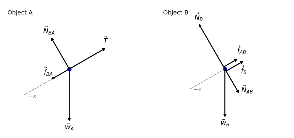
../_images/8b2e9276d0846414f966cbb454bdd0964a51c6e35ed192916d01c6e4221e6446.png

5.7.2. Example Problem: Two Blocks in Contact#

Exercise 5.15

The Problem

A force is applied to two blocks in contact, as shown in Fig. 5.26. Draw the reaction forces between the two blocks.

2 blocks contact FBD example — Fig. 5.26 Image Credit: OpenStax: Drawing Free-body Diagrams#

Show code cell source Hide code cell source

import numpy as np
import matplotlib.pyplot as plt

# -----------------------------
# draw_fbd helper 
# -----------------------------
def draw_fbd(ax, forces, labels, note, colors=None):
    ax.plot(0, 0, "k.", markersize=14)
    if colors is None:
        colors = ["black"] * len(forces)
    for F, lab, col in zip(forces, labels, colors):
        Fx, Fy = F
        ax.annotate("", xy=(Fx, Fy), xytext=(0, 0),
                    arrowprops=dict(arrowstyle="->", lw=2, color=col,shrinkA=0, shrinkB=0))
        ax.annotate(lab, xy=(Fx, Fy), xytext=(6, 6),textcoords="offset points",
            fontsize=13, color=col, ha="left", va="bottom")
    mags = [np.hypot(F[0], F[1]) for F in forces]
    R = 1.35 * max(mags + [1.0])
    ax.set_xlim(-R, R)
    ax.set_ylim(-R, R)
    ax.set_aspect("equal", adjustable="box")
    ax.set_xticks([])
    ax.set_yticks([])
    for spine in ax.spines.values():
        spine.set_visible(False)
    ax.text(0.03, 0.95, note, transform=ax.transAxes,fontsize=12, va="top")
# -----------------------------
# Scaled forces for clarity
# -----------------------------
F_applied = 1.2   # applied force on block 1 (to the right)
A = 0.8           # interface force magnitude (same for the pair)
# Reaction pair:
# A_21 = force on block 1 due to block 2 (left)
# A_12 = force on block 2 due to block 1 (right)
A21 = np.array([-A, 0.0])
A12 = np.array([+A, 0.0])
# Optional vertical context (not required by the prompt)
N1 = np.array([0.0, 1.0])
w1 = np.array([0.0, -1.0])
N2 = np.array([0.0, 1.0])
w2 = np.array([0.0, -1.0])
# Block 1 FBD (shows applied force + reaction from block 2)
forces_1 = [np.array([F_applied, 0.0]), A21, N1, w1]
labels_1 = [r"$\vec{F}$", r"$\vec{A}_{21}$", r"$\vec{N}_1$", r"$\vec{w}_1$"]
colors_1 = ["tab:red", "tab:red", "k", "k"]
# Block 2 FBD (shows reaction from block 1)
forces_2 = [A12, N2, w2]
labels_2 = [r"$\vec{A}_{12}$", r"$\vec{N}_2$", r"$\vec{w}_2$"]
colors_2 = ["tab:red", "k", "k"]
# -----------------------------
# Plot
# -----------------------------
fig, axes = plt.subplots(1, 2, figsize=(8, 4), dpi=120)

draw_fbd(axes[0], forces_1, labels_1, "Block $m_1$", colors=colors_1)
draw_fbd(axes[1], forces_2, labels_2, "Block $m_2$", colors=colors_2)

plt.tight_layout()
plt.show()

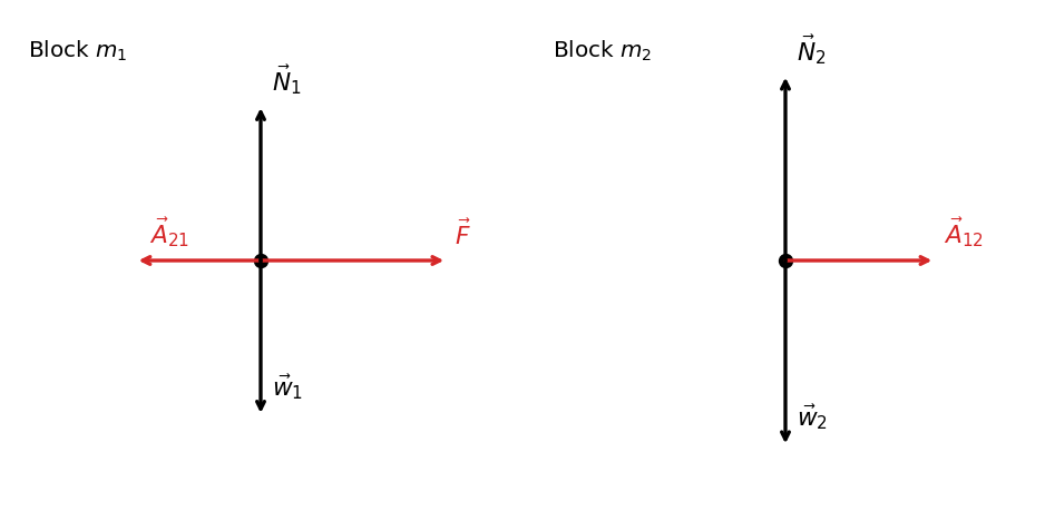
../_images/50dca658772a822df8de66e6b47c36bb872bd2dacec5bdd3d7ccf846e8b221a3.png

5.7.3. Example Problem: Block on the Table#

Exercise 5.16

The Problem

A block rests on the table, as shown in Fig. 5.26. A light rope is attached to it and runs over a pulley. The other end of the rope is attached to a second block. The two blocks are said to be coupled. Block $m_2$ exerts a force due to its weight, which causes the system (two blocks and a string) to accelerate.

We assume that the string has no mass so that we do not have to consider it as a separate object. Draw a free-body diagram for each block.

2 blocks pulley FBD example — Fig. 5.27 Image Credit: OpenStax: Drawing Free-body Diagrams#

The Model

The two blocks are treated as separate systems connected by a taut, massless rope over a frictionless pulley. For block $m_1$, the positive $x$ direction is to the right, toward the pulley, and the positive $y$ direction is upward. For block $m_2$, the positive $y$ direction is upward. The table is treated as frictionless, so no friction force acts on $m_1$. The rope tension has the same magnitude on both blocks.

The Math

To construct the free-body diagrams, each block is isolated and only forces acting on that block are included.

For block $m_1$, the weight $\vec{w}_1$ acts downward, the normal force $\vec{N}$ from the table acts upward, and the rope tension $\vec{T}$ acts horizontally to the right toward the pulley.

For block $m_2$, the weight $\vec{w}_2$ acts downward and the rope tension $\vec{T}$ acts upward. The tension has the same magnitude in both diagrams because the rope is massless and the pulley is frictionless.

Apply Newton’s second law separately to each block, using $+x$ to the right for $m_1$ and $+y$ upward for $m_2$.

For block $m_1$, we have for the horizontal motion

\[\begin{align*} \sum F_x &= m_1 a \\ T &= m_1 a . \end{align*}\]

For block $m_1$ in the vertical direction,

\[\begin{align*} \sum F_y &= 0 \quad \text{(no vertical acceleration)}\\ N - m_1 g &= 0 \\ N &= m_1 g . \end{align*}\]

For block $m_2$, we have for the vertical motion,

\[\begin{align*} \sum F_y &= m_2 a_y \\ T - m_2 g &= m_2(-a) \\ m_2 g - T &= m_2 a . \end{align*}\]

Then, we can solve the two acceleration–tension equations for $a$ in terms of $T$:

\[\begin{align*} T &= m_1 a \\ m_2 g - T &= m_2 a. \end{align*}\]

Then, we can solve for $a$ and $T$ separately in terms of the masses and $g$:

\[\begin{align*} m_2 g - m_1 a &= m_2 a \\ a &= \frac{m_2 g}{m_1 + m_2}, \\ T &= m_1\left(\frac{m_2 g}{m_1 + m_2}\right)\\ &= \frac{m_1 m_2 }{m_1 + m_2} g. \end{align*}\]

The Conclusion

The free-body diagram for $m_1$ contains $\vec{N}$ upward, $\vec{w}_1$ downward, and $\vec{T}$ to the right. The free-body diagram for $m_2$ contains $\vec{T}$ upward and $\vec{w}_2$ downward. The two blocks require separate free-body diagrams because the forces acting on each block are different, even though their accelerations are linked by the rope.

Because the rope is massless and taut over a frictionless pulley, the tension magnitude is the same on both blocks and the acceleration magnitudes are equal:

\[\begin{align*} a &= \frac{m_2 g}{m_1+m_2},\\ \\ T &= \frac{m_1 m_2 g}{m_1+m_2}. \end{align*}\]

The Organic Chemistry Tutor

This video gives another worked example of a pulley system, emphasizing separate free-body diagrams, shared tension, and the acceleration constraint.

The Verification

The Python check in the next cell draws schematic free-body diagrams for both blocks. The purpose is to verify that the correct forces appear on each isolated block, not to solve for the acceleration or tension.

Show code cell source Hide code cell source

import numpy as np
import matplotlib.pyplot as plt

# -----------------------------
# Helper: draw_fbd 
# -----------------------------
def draw_fbd(ax, forces, labels, note, colors=None, offsets=None):
    ax.plot(0, 0, "b.", markersize=15)
    if colors is None:
        colors = ["black"] * len(forces)
    if offsets is None:
        offsets = [np.array([0.0, 0.0])] * len(forces)
    for F, lab, col, off in zip(forces, labels, colors, offsets):
        Fx, Fy = F
        ox, oy = off
        ax.annotate("", xy=(Fx + ox, Fy + oy), xytext=(ox, oy),arrowprops=dict(arrowstyle="->", lw=2, color=col, shrinkA=0, shrinkB=0))
        # Label a little past the tip, in display coordinates
        ax.annotate(lab, xy=(Fx + ox +1, Fy + oy), xytext=(8, 6),textcoords="offset points", color=col, fontsize=14,ha="center", va="center")
    mags = [np.hypot(F[0] + off[0], F[1] + off[1]) for F, off in zip(forces, offsets)]
    R = 1.35 * max(mags + [1.0])
    ax.set_xlim(-R, R)
    ax.set_ylim(-R, R)
    ax.set_aspect("equal", adjustable="box")
    ax.set_xticks([])
    ax.set_yticks([])
    for spine in ax.spines.values():
        spine.set_visible(False)
    ax.text(0.03, 0.95, note, transform=ax.transAxes, fontsize=12, va="top")
# -----------------------------
# Parameters (sample check)
# -----------------------------
m1 = 3.0   # kg
m2 = 2.0   # kg
g  = 9.81  # m/s^2

a = (m2 * g) / (m1 + m2)
T = m1 * a

print(f"The sample mass on the table is {m1:.3g} kg.")
print(f"The sample hanging mass is {m2:.3g} kg.")
print(f"The computed acceleration magnitude is {a:.3g} m/s^2.")
print(f"The computed rope tension is {T:.3g} N.")

# -----------------------------
# Forces for each block (scaled to real magnitudes)
# Use plot-units = N, then autoscale by draw_fbd.
# -----------------------------
# Block m1 on table
w1 = np.array([0.0, -m1*g])
N  = np.array([0.0,  m1*g])
T1 = np.array([T, 0.0])
forces_m1 = [N, w1, T1]
labels_m1 = [r"$\vec{N}$", r"$\vec{w}_1$", r"$\vec{T}$"]
colors_m1 = ["k", "k", "k"]
offsets_m1 = [[0,0],[0,0],[0,0]]
# Block m2 hanging
w2 = np.array([0.0, -m2*g])
T2 = np.array([0.0,  T])
forces_m2 = [T2, w2]
labels_m2 = [r"$\vec{T}$", r"$\vec{w}_2$"]
colors_m2 = ["k", "k"]
offsets_m2 = [[0,0],[0,0],[0,0]]

# -----------------------------
# Plot
# -----------------------------
fig, axes = plt.subplots(1, 2, figsize=(7, 3.8), dpi=120)

draw_fbd(axes[0], forces_m1, labels_m1, r"Block $m_1$", colors=colors_m1,offsets=offsets_m1)
draw_fbd(axes[1], forces_m2, labels_m2, r"Block $m_2$", colors=colors_m2,offsets=offsets_m2)

plt.tight_layout()
plt.show()

The sample mass on the table is 3 kg.
The sample hanging mass is 2 kg.
The computed acceleration magnitude is 3.92 m/s^2.
The computed rope tension is 11.8 N.

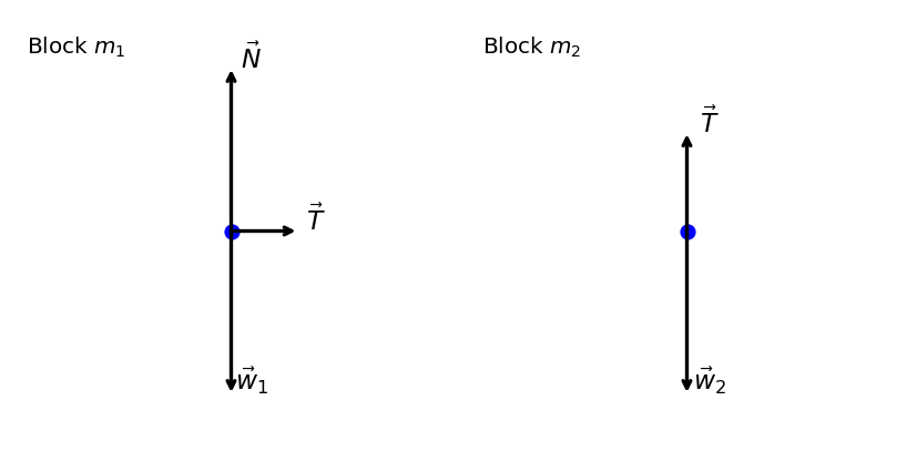
../_images/15e06d9ba98fe577398f0bc9e99afb18f94f1c13d2569d76442b7f1b2dc6d918.png

5.8. In-class Problems#

5.8.1. Part I#

Problem 1

Two ropes are attached to a tree, and forces of $\vec{F}_1 = 2.0\hat{i} + 4.0\hat{j}\ \text{N}$ and $\vec{F}_2 = 3.0\hat{i} + 6.0\hat{j}\ \text{N}$ are applied. The forces are coplanar (in the same plane).

(a) What is the resultant (net force) of these two force vectors? (b) Find the magnitude and direction of this net force.

Problem 2

A cleaner pushes a $4.50\ \text{kg}$ laundry cart in such a way that the net external force on it is $60.0\ \text{N}$. Calculate the magnitude of the cart’s acceleration.

Problem 3

In the following figure, the horizontal surface on which this block slides is frictionless. If the two forces acting on it each have magnitude $F = 30.0\ \text{N}$ and $M = 10.0\ \text{kg}$, what is the magnitude of the resulting acceleration of the block?

force block problem — Fig. 5.28 Image Credit: OpenStax: Chapter 5 Problems#

Problem 4

Suppose the mass of a fully loaded module in which astronauts take off from the Moon is $1.00 \times 10^4\ \text{kg}$. The thrust of its engines is $3.00 \times 10^4\ \text{N}$.

(a) Calculate the module’s magnitude of acceleration in a vertical takeoff from the Moon. (b) Could it lift off from Earth? If not, why not? If it could, calculate the magnitude of its acceleration.

5.8.2. Part II#

Problem 5

(a) What net external force is exerted on a $1100.0\ \text{kg}$ artillery shell fired from a battleship if the shell is accelerated at $2.40 \times 10^4\ \text{m/s}^2$?
(b) What is the magnitude of the force exerted on the ship by the artillery shell, and why?

Problem 6

(a) Calculate the tension in a vertical strand of spider web if a spider of mass $2.00 \times 10^{-5}\ \text{kg}$ hangs motionless on it.

(b) Calculate the tension in a horizontal strand of spider web if the same spider sits motionless in the middle of it much like the tightrope walker in Figure 5.21. The strand sags at an angle of $12^\circ$ below the horizontal. Compare this with the tension in the vertical strand (find their ratio).

Problem 7

A $2.0\ \text{kg}$ block is on a perfectly smooth ramp that makes an angle of $30^\circ$ with the horizontal.

(a) What is the block’s acceleration down the ramp and the force of the ramp on the block? (b) What force applied upward along and parallel to the ramp would allow the block to move with constant velocity?

Problem 8

The traffic light hangs from the cables as shown. Draw a free-body diagram on a coordinate plane for this situation.

traffic light problem — Fig. 5.29 Image Credit: OpenStax: Chapter 5 Problems#

5.9. Homework#

5.9.1. Conceptual Problems#

Problem 1

A rock is thrown straight up. At the top of the trajectory, the velocity is momentarily zero. Does this imply that the force acting on the object is zero? Explain your answer.

Problem 2

How much does a 70-kg astronaut weigh in interstellar space, far from any celestial body? What is her mass at this location?

5.9.2. Quantitative Problems#

Problem 3

A particle of mass $2.0\ \mathrm{kg}$ is acted on by a single force $\vec{F}_1 = 18\hat{i}\ \mathrm{N}$.

(a) What is the particle’s acceleration?
(b) If the particle starts at rest, how far does it travel in the first $5.0\ \mathrm{s}$?

Problem 4

A rugby player is being pushed backward by an opposing player who is exerting a force of $800.0\ \mathrm{N}$ on him. The mass of the losing player plus equipment is $90.0\ \mathrm{kg}$, and he is accelerating backward at $1.20\ \mathrm{m/s^2}$.

(a) What is the force of friction between the losing player’s feet and the grass?
(b) What force does the winning player exert on the ground to move forward if his mass plus equipment is $110.0\ \mathrm{kg}$?

Problem 5

A truck collides with a car, and during the collision, the net force on each vehicle is essentially the force exerted by the other. Suppose the mass of the car is $550\ \mathrm{kg}$, the mass of the truck is $2200\ \mathrm{kg}$, and the magnitude of the truck’s acceleration is $10\ \mathrm{m/s^2}$. Find the magnitude of the car’s acceleration.

Problem 6

A bird has a mass of $26\ \mathrm{g}$ and perches in the middle of a stretched telephone line.

(a) Show that the tension in the line can be calculated using the equation

\[ T = \frac{mg}{2\sin\theta}.\]

Determine the tension when
(b) $\theta = 5^\circ$ and
(c) $\theta = 0.5^\circ$.

Assume that each half of the line is straight.

Problem 7

A ball of mass $m$ hangs at rest, suspended by a string.

(a) Sketch all forces acting on the ball.
(b) Draw the free-body diagram for the ball.

Newton’s Laws of Motion

Contents

5. Newton’s Laws of Motion#

5.1. Forces#

5.1.1. Working Definition of Force#

5.1.2. Contact and Field Forces#

5.1.3. Vector Notation for Force#

5.2. Newton’s 1st Law#

5.2.1. Gravitation and Inertia#

5.2.2. Inertial Reference Frames#

5.2.3. Newton’s 1st Law and Equilibrium#

5.2.3.1. Example Problem: Applying Newton’s 1st Law to your car#

5.3. Newton’s 2nd Law#

5.3.1. Force and Acceleration#

5.3.1.1. Example Problem: Pushing a Lawnmower#

5.3.1.2. Example Problem: Comparing Forces#

5.3.1.3. Example Problem: Thrust on a Sled#

5.3.2. Component Form of Newton’s 2nd Law#

5.3.2.1. Example Problem: Force on a Soccer Ball#

5.3.2.2. Example Problem: Mass of a Car#

5.3.2.3. Example Problem: Several Forces#

5.3.3. Newton’s 2nd Law and Momentum#

5.4. Mass and Weight#

5.4.1. Units of Force#

5.4.2. Weight and Gravitational Force#

5.4.2.1. Example Problem: Lifting a Stone#

5.5. Newton’s 3rd Law#

5.5.1. Example Problem: Forces on a Stationary Object#

5.5.2. Example Problem: Force on the Cart (Part 1)#

5.5.3. Example Problem: Force on the Cart (Part 2)#

5.6. Common Forces#

5.6.1. Normal Force#

5.6.1.1. Example Problem: Weight on an incline#

5.6.2. Tension#

5.6.2.1. Example Problem: Tension in a Tightrope#

5.6.3. Friction#

5.6.4. Spring Force#

5.6.5. Real Forces and Inertial Frames#

5.7. Drawing Free-body Diagrams#

5.7.1. Example Problem: Two Blocks on an Inclined Plane#

5.7.2. Example Problem: Two Blocks in Contact#

5.7.3. Example Problem: Block on the Table#

5.8. In-class Problems#

5.8.1. Part I#

5.8.2. Part II#

5.9. Homework#

5.9.1. Conceptual Problems#

5.9.2. Quantitative Problems#