1. Units and Measurement#
Jul 20, 2026 | 6607 words | 44 min read
Chapter roadmap
This chapter introduces the measurement tools used throughout physics: units, conversion factors, dimensional analysis, uncertainty, and significant figures.
As you read, focus on three questions:
Can I track units through a calculation?
Can I tell whether an equation is dimensionally consistent?
Can I report a numerical answer with appropriate precision?
These skills will be used repeatedly in homework, labs, and exams.
1.1. Scope and Scale of Physics#
This narration is AI-generated from the course text.
1.1.1. What is physics?#
Physics is a method to better understand all natural phenomena. Physicists try to understand our physical universe, starting from the very small up to (and including) the entire universe. The same basic training can be applied in many areas of science and engineering, where there can be significant overlap across disciplines. If something changes in time, there’s a discipline dedicated to understanding how and why it changes.
Physics, which derives from the Greek word for “nature,” is the science concerned with describing the fundamental interactions of energy, matter, space, and time. It seeks to understand the world at its most basic level by using a small number of quantitative laws.
This approach reveals deep connections between seemingly unrelated topics, such as how the law of conservation of energy applies to both a car battery and a bag of chips. By focusing on these underlying laws, the study of physics provides a framework for understanding that goes beyond memorization and helps develop strong analytical and problem-solving skills.
1.1.2. The Scope of Physics#
1.1.2.1. In the Universe#
The universe contains trillions of galaxies, which are megastructures compared to our own Solar System. How can we comprehend how big they are? Or how they operate?

Fig. 1.1 The Whirlpool Galaxy (M51), observed by the James Webb Space Telescope, showing detailed spiral arms, dust lanes, and regions of active star formation. Astronomical images like this are constructed from measurements of light collected across multiple wavelengths and scales, illustrating how physical quantities and units underpin observational astronomy. Image Credit: NASA / ESA / CSA / STScI.#
The Whirlpool Galaxy (or M51) lies 31 million lightyears away from us. This is an astoundingly large distance. We can use this as a starting point to raise the question about how we put this into perspective.
Think of the distances to various places.
The distance across the USA is about \(4500\ {\rm km}\) from east to west. This seems like a long way, but the distance from the Earth to the Sun (or astronomical unit; AU) is about \(149,000,000\ {\rm km}\) or \({\sim}33,000\times\) more distant. Light is incredibly fast and can travel 1 AU in only \(8.3\ {\rm min}\).
How far can light travel in a year?
Instead of thinking in kilometers, it is simpler to instead describe this distance in AU, or how many Earth-Sun distances make up this proposed distance. We have to give this distance a name, thus we call it a lightyear, or the distance that light travels in a year. Let’s start with what we know so far (i.e., light travels 1 AU in 8.3 min):
Therefore, light travels at a speed of about \(0.12\ {\rm AU/min}\). Now, we can work our way through if we can somehow translate this speed into a distance. For this we can use some other knowledge, for example:
These are the conversion factors that we need to start unpacking the speed of light and to determine how far it can travel in a year. We can use a technique called dimensional analysis to combine these factors to achieve our goal.
To understand the distance \(d\) in a lightyear, we need to convert its speed \(s\) using different timescales \(t\) that make up a year.
Let’s begin with some analytical calculations, which we’ll follow-up with a verification using python. We just need to use our known speed of light and multiply by different time conversion factors to determine the number of \(\rm AU/yr\), or
Note
You can express math terms more easily using math mode in a Markdown (or text) cell of your Jupyter notebook. The math mode uses LaTeX commands that are entered programmatically and rendered once you escape a cell. For example, the area of a circle is $A = \pi r^2$ is rendered as \(A = \pi r^2\).
You can express multi-line equations using the \begin{align} \end{align} environment, where each line is aligned using the & symbol. Open this page in Google Colab and view the source for more examples.
Here’s an example of the calculation using python, where you should note the comments so that it is understandable by future-you.
import numpy as np #import statement to use numpy functions

s = 0.12 #speed of light in AU/min
min2hr = 60 #number of minutes in an hour
hr2day = 24 #number of hours in a day
day2yr = 365.25 #number of days in a year

s = s*min2hr*hr2day*day2yr
print("The speed of light is %4.0f AU/yr." % s)
print("-------")
print("Note this is not accurately describing our calculation.  We are limited by the precision of s.")
print("-------")
print("The speed of light is %4.0f AU/yr." % np.round(s,-3))
The speed of light is 63115 AU/yr.
-------
Note this is not accurately describing our calculation.  We are limited by the precision of s.
-------
The speed of light is 63000 AU/yr.
We’ve found that the speed of light is about \(63,000\ {\rm AU/yr}\). Now we can determine the distance in a lightyear, which is
We have arrived at our goal, which is \(1\ {\rm ly} = 63{,}000\ {\rm AU}\).
Checkpoint
A lightyear is a unit of distance, not time.
Why does multiplying a speed by a time produce a distance?
Why do we want to know this?
It shows us that a lightyear is really big, or \(63,000\times\) the distance from the Earth to the Sun. Then, it shows that the distance to M51 is even bigger, meaning that it is 31 million times farther away than something that is only 1 lightyear away.
Moreover, M51 is composed of billions of stars where these stars interact in a complex way that we can actually understand (to some degree). For now, we posit that the force holding the galaxies together is the same as the one holding you onto the Earth.
1.1.2.2. On the Earth#
Humans have been remarkable at creating new gadgets and tools. This process is marked by our ability to identify and manipulate certain materials so that we can bend them to our own purposes. This knowledge stems from physics, where our current technological prowess has produced a way for you to acquire the sum of all knowledge and carry it with you in your pocket.
A key innovation to producing your phone is the MOSFET transistor and forms the basis of all modern electronics. Physics also underpins complex systems like GPS and continues to drive future technologies like levitating trains and microscopic medical robots. Furthermore, physics explains the function of everyday items, such as how a microwave oven works or why a black car radiator helps remove heat.
Because physics is a foundational science, its principles are essential across a wide range of professions and scientific fields.
Professionals such as pilots, engineers, physical therapists, and computer programmers apply physics concepts in their daily work.
Physics is also a key element in other disciplines, including chemistry, architecture, and geology.
It has critical applications in biology and medicine, explaining phenomena from the properties of cells to the mechanics of the human body, and enabling crucial diagnostic tools like MRIs, radiographs, and ultrasonic imaging.
1.1.3. The Scale of Physics#
The laws of physics operate at all measurable scales of length, mass, and time. To think on such scales, scientists use the concept of “order of magnitude” because it provides an approximation for that scale that guides our thinking or intuition. The breadth of physics is not limited to the mechanics of the 19th century, but has been the fuel of progress for the last 150 years and is expected to continue yielding returns into the future with AI.
The next wave [of AI] requires us to understand things like the laws of physics, friction, inertia, and cause and effect.
—Jensen Huang, Nvidia CEO
1.1.3.1. Order of magnitude#
The order of magnitude describes a number to the closest power of \(10\). Thus, it refers directly to the scale (or size) of the value. To find the order of magnitude, we have two options:
take the base-\(10\) logarithm of the number, then raise the whole number part to a power of \(10\). For example,
\[\begin{align*} \log_{10}{250} &= 2.40 \approx \mathbf{2} \rightarrow 10^\mathbf{2},\\ \log_{10}{450} &= 2.65 \approx \mathbf{3} \rightarrow 10^\mathbf{3}, \\ \log_{10}{12345} &= 4.09 \approx \mathbf{4} \rightarrow 10^\mathbf{4}. \end{align*}\]write the number in scientific notation and then check to see whether the first factor is greater or less than \(\sqrt{10} \approx 3\). The
square rootcan be expressed as a fractional power so that \(\sqrt{10} = 10^{1/2}\) so that we are estimating the halfway point between powers. For example,\[\begin{align*} 250 &= 2.5 \times 10^\mathbf{2}; \quad 2.5<3 \rightarrow 10^\mathbf{2},\\ 450 &= 4.5 \approx 10^2; \quad 4.5 > 3 \rightarrow 10^\mathbf{2+1} = 10^{3}, \\ 12345 &= 1.2345 \times 10^\mathbf{4}; \quad 1.2345 < 3 \rightarrow 10^\mathbf{4}. \end{align*}\]
The order of magnitude is a ballpark estimate for the scale (or size) of its value, where it rounds the numbers consistently to the nearest power of 10 on a logarithmic scale. This makes doing mental arithmetic easier when dealing with very small or large numbers.
The diameter of the hydrogen atom is \({\sim}10^{-15}\ {\rm m}\), whereas the diameter of the Milky Way Galaxy is \({\sim}10^{21}\ {\rm m}\). It would take \(10^{21}/10^{-15} = 10^{36}\) hydrogen atoms to stretch across our Galaxy. It’s much easier to do in your head (or on the back of an envelope) if you can ignore the first factor in the more precise number.
Checkpoint
Which number has order of magnitude \(10^3\)?
\(250\), \(450\), or \(12345\)?
1.1.3.2. Known ranges of length, mass, and time#
Figure 1.2 shows a wide range of examples of known lengths, masses, and times given by their order of magnitude. Consider the following:
How many protons are there in a bacterium?
How many floating-point operations can a super computer do in a day?
Formatting equations and units
The above calculation uses $$ $$ as a shorthand environment that centers an equation without numbering it. It requires a blank line before and after so that it renders properly.
To add space between the value and unit, use
\␣(backslash + space).To express the unit, place it in curly braces with
\rm␣preceding the unit (e.g.{\rm kg}renders as \({\rm kg}\)), or use the\text{}command (e.g.\text{kg}renders as \(\text{kg}\)).To express a superscript or subscript, use
^{}or_{}, respectively, e.g.10^{12}renders as \(10^{12}\).
Equations are part of sentences, be sure to use the appropriate punctuation (i.e., , or ‘.’) to include them seamlessly.
Fig. 1.2 This table shows the orders of magnitude of length, mass, and time. Figure Credit: OpenStax: Scope and Scale of Physics.#
1.1.4. Building Models#
The universe is very complicated, where it can be quite daunting to try understanding it fundamentally with every possible interaction included. As a result, we make human statements of the underlying laws or rules that all natural processes follow. Such laws are intrinsic to the universe; humans did not create them and cannot change them. We can only discover and understand them.
1.1.4.1. What is a model?#
A model is a representation of something that is often too difficult to describe fully. It is only accurate in describing certain aspects of a physical system. Consider the following joke about spherical cows:
Milk production at a dairy farm was low, so the farmer wrote to the local university, asking for help from academia. A multidisciplinary team of professors was assembled, headed by a theoretical physicist, and two weeks of intensive on-site investigation took place. The scholars then returned to the university, notebooks crammed with data, where the task of writing the report was left to the team leader. Shortly thereafter the physicist returned to the farm, saying to the farmer, “I have the solution, but it works only in the case of spherical cows in a vacuum.
The inner workings of a cow or its complex shape are too difficult to describe with simple equations. So the theoretical physicist makes a simplifying assumption that a cow can be modeled as a sphere and air resistance can be neglected (i.e., in a vacuum).
In the beginning stages of quantum mechanics, the Bohr model of single-electron atoms provided a “good-enough” mental image to explain some of the observations that we can make (e.g., atomic spectra).
Interactive Simulation: Hydrogen Atom Models
Use this PhET simulation to explore classical, Bohr, and quantum models of the hydrogen atom. Adjust parameters and observe how predicted electron behavior differs between models.
However other observations show that the model is “wrong”, but is still useful for some purposes. Models are useful to help physicists analyze a scenario, perform a calculation, or investigate different situations via a computer simulation. The results of these calculations and simulations always need to be double-checked by observation and/or experimentation.
1.1.4.2. Theory vs. law#
The word theory can have a different meaning depending on the context, where the layman uses it interchangeably with “hypothesis”. In particular, a scientific theory is not the same as a hypothesis, where it is instead:
a
testableexplanation for patterns in nature supported by evidence and verified multiple times by independent researchers.
Newton’s theory of gravity does not require a model or mental image because it describes objects or events directly available to our senses. Quantum theory, on the other hand, does require a mental model or picture.
A theory should describe all aspects of any system that falls within its applicable domain and any experimentally testable implication of a theory should be verified.
A law uses concise language to describe a generalized pattern in nature supported by scientific experiments and repeated experiments. Often a law is expressed by a mathematical equation. Laws and theories are similar in that they both are scientific statements that result from a tested hypothesis and are supported by scientific evidence.
The designation of law is usually reserved for a concise and very general statement that describes phenomena in nature (e.g., energy is conserved in any process or force is related to mass times acceleration, \(\vec{F}=m\vec{a}\).)
A theory is a less concise statement of observed behavior. For example, the theory of evolution and theory of special relativity cannot be expressed concisely enough to be considered laws.
A theory explains an entire group of phenomena, whereas a law describes a single action.
Less broadly applicable statements are usually called principles (e.g., Pascal’s principle is applicable to only fluids), but the distinction between laws and principles often is not carefully made.
If it disagrees with experiment, it’s wrong. In that simple statement is the key to science. It doesn’t make any difference how beautiful your guess is. It doesn’t make any difference how smart you are, who made the guess, or what his name is. If it disagrees with experiment, it’s wrong.
—Richard Feynman, Caltech Lectures
Richard Feynman Lectures
1.2. Units and Standards#
This narration is AI-generated from the course text.
A physical quantity is defined by specifying how it is measured or how it is calculated from other measurements. For example,
distance measured using a meter stick, or time measured with a stopwatch,
average speed is the total distance traveled divided by the travel time.
Measurements of physical quantities are expressed in terms of standardized units. The foot was part of many local systems of units, but it was not standardized until 1959. It varied in length from city to city and even from trade to trade. Therefore, it’s important to have a standardized length (e.g., meter) so that international science or manufacturing can operate smoothly.
Two major units are used in the world:
SI units (for the French Système International d’Unités) or metric system, and
English units (i.e., the imperial system).
Systems of units are also referred to by just listing what they use for length-mass-time (e.g., foot-pound-second or meter-kilogram-second). The metric system is agreed on by scientists and mathematicians. Engineers may use SAE (Society of Automotive Engineers) units that measure tools in fractions of an inch rather than millimeters.
1.2.1. SI Units: Base and Derived Units#
The base quantities are measured using a system’s base units. All other physical quantities are combinations of the base quantities, where each are known as a derived quantity with its own derived unit. The derived units can only be as accurate and precise as the base units from which they are derived.
There are \(7\) base units that make up the international System of Quantities (ISQ). Table 1.1 lists the units corresponding to the ISQ base quantities.
ISQ Base Quantity |
SI Base Unit |
Common Imperial / U.S. Customary Unit |
|---|---|---|
Length |
meter (m) |
foot (ft) |
Mass |
kilogram (kg) |
pound-mass (lbm) |
Time |
second (s) |
second (s) |
Electric current |
ampere (A) |
ampere (A) |
Thermodynamic temperature |
kelvin (K) |
degree Fahrenheit (\(^\circ\)F) |
Amount of substance |
mole (mol) |
— (no Imperial base unit) |
Luminous intensity |
candela (cd) |
candlepower (cp, historical) |
Examples of derived units are expressed as:
area; \(\rm m^2\),
volume; \(\rm m^3\) or \(\rm cc = cm^3 = mL\) (in fluids)
speed; \(\rm m/s\),
density; \(\rm kg/m^3\),
electric charge; \(\rm A\cdot s\),
energy; \(\rm eV\) (electron-Volts).
1.2.2. Units of Time, Length, and Mass#
1.2.2.1. The second#
For many years the second was defined as \(1/86,400\) of a mean solar day. A new standard was introduced to define the second in terms of a nonvarying physical phenomenon because the lunar and solar tides cause the Earth’s rotation to slow over time.
Cesium atoms can vibrate in a steady way, allowing them to be easily observed and counted. In 1967, the second was redefined as the time required for \(9,192,631,770\) of these vibrations to occur. This level of precision is needed for global position satellites (GPSs) to give you turn-by-turn directions due to time dilation in relativity.
1.2.2.2. The meter#
The meter has changed its definition over time (like the second) to become more precise.
The meter was first defined in 1791 as \(1/10^7\) of the distance from the equator to the North Pole.
The measurement was improved in 1889 by redefining the meter as the distance between 2 engraved lines on a bar of \(\rm Pt\text{-}Ir\) (kept in Paris).
In 1960, it was redefined again as \(1,650,763.73\) wavelengths of light emitted by \(\rm Kr\) atoms.
In 1983, the meter was given its current definition as the distance light travels (in a vacuum) in \(1/299,792,458\) of a second (or \(1/c\))
1.2.2.3. The kilogram#
The kilogram was defined from 1795-2018 as the mass of a platinum-iridium (\(\rm Pt\text{-}Ir\)) cylinder kept in Paris. However, this cylinder has lost roughly \(50\ {\rm \mu g}\) since it was created.
In May 2019, the new definition was based on physical constants of the universe (e.g., Planck constant). The kilogram is now measured using a Kibble balance, which measures an electrical current produced that is proportional to Planck’s constant. Using the exact definition of the Planck constant, this means that the exact measurement of the current can define the kilogram.
1.2.3. Metric Prefixes#
The “beauty” of the metric system is its convenience for categorizing units by factors of \(10\). Table 1.2 lists the metric prefixes and symbols used to denote various factors of \(10\) in SI units. For example,
a centimeter is \(1/100\) of a meter (\(1\ {\rm cm}=10^{-2}\ {\rm m}\)),
a kilometer is \(1000\) meters (\(1\ {\rm km} = 10^3\ {\rm m}\)),
a nanosecond is 1/billionth of a second (\(1\ {\rm ns} = 10^{-9}\ {\rm s}\)).
Prefix |
Symbol |
Meaning |
Prefix |
Symbol |
Meaning |
|---|---|---|---|---|---|
yotta- |
Y |
\(10^{24}\) |
yocto- |
y |
\(10^{-24}\) |
zetta- |
Z |
\(10^{21}\) |
zepto- |
z |
\(10^{-21}\) |
exa- |
E |
\(10^{18}\) |
atto- |
a |
\(10^{-18}\) |
peta- |
P |
\(10^{15}\) |
femto- |
f |
\(10^{-15}\) |
tera- |
T |
\(10^{12}\) |
pico- |
p |
\(10^{-12}\) |
giga- |
G |
\(10^{9}\) |
nano- |
n |
\(10^{-9}\) |
mega- |
M |
\(10^{6}\) |
micro- |
\(\mu\) |
\(10^{-6}\) |
kilo- |
k |
\(10^{3}\) |
milli- |
m |
\(10^{-3}\) |
hecto- |
h |
\(10^{2}\) |
centi- |
c |
\(10^{-2}\) |
deka- |
da |
\(10^{1}\) |
deci- |
d |
\(10^{-1}\) |
The only rule when using the metric prefixes is that you cannot “double them up”. For example, it is improper to talk about megagigameters, although \(10^6 \times 10^9 = 10^{15}\) (\(1\ {\rm Pm} = 10^{15}\ {\rm m}\)).
Checkpoint
Which is the better metric-prefix form?
\(0.0042\ {\rm g}\) or \(4.2\ {\rm mg}\)?
Why?
1.2.3.1. Example Problem: Metric Prefixes#
Exercise 1.1
The Problem
Restate the mass \(1.93 \times 10^{13}\ {\rm kg}\) using a metric prefix such that the resulting numerical value is bigger than one but less than 1000.
The Model
We treat mass as a scalar physical quantity expressed as a numerical value multiplied by a unit. Metric prefixes encode powers of ten and may not be combined or “stacked.” Therefore, the mass must first be rewritten using explicit powers of ten before introducing a single appropriate prefix.
Our goal is to select a metric prefix that produces a numerical value between 1 and 1000 while representing the same physical mass.
The Math
The prefix kilo- corresponds to a factor of \(10^{3}\). Rewriting the mass in grams gives
From Table 1.2, the power \(10^{16}\) lies between
peta- (\(10^{15}\)), and
exa- (\(10^{18}\)).
If we factor out \(10^{15}\), we obtain
Alternatively, factoring out \(10^{18}\) gives
which produces a numerical value less than one and therefore does not satisfy the requirement of the problem.
The Conclusion
The mass expressed using a single metric prefix with a numerical value between 1 and 1000 is
The Verification
We can verify this conversion numerically by explicitly tracking the powers of ten using Python (see below).
This output confirms that \(1.93 \times 10^{13}\ {\rm kg} = 19.3\ {\rm Pg}\), matching the analytical result. Comparing powers of ten also shows consistency: (13 + 3 = 1 + 15 = 16).
For additional physical context, the scale of this mass can be compared to common mass benchmarks shown in Figure 1.2.
# Given mass in kilograms
mass_kg = 1.93e13

# Convert kilograms to grams
mass_g = mass_kg * 1e3

# Convert grams to petagrams (1 Pg = 1e15 g)
mass_pg = mass_g / 1e15

print(f"Mass in grams: {mass_g:.2e} g")
print(f"Mass in petagrams: {mass_pg:.1f} Pg")
Mass in grams: 1.93e+16 g
Mass in petagrams: 19.3 Pg
1.3. Unit Conversion#
This narration is AI-generated from the course text.
It is often necessary to convert from one unit to another (as you’ve already seen). If you are reading a cookbook, some quantities may be expressed in milliliters and you need to convert them to cups.
Suppose we want to convert \(80\ {\rm m}\) to kilometers.
Start with the input value you want to convert as a fraction (i.e., itself over one).
Determine the conversion factor necessary. A conversion factor is a ratio that describes how much of one unit is equal to another.
Multiply by the ratio so that unit from the input value cancels (i.e., \(\rm unit/unit = 1\)).
Using these steps, we have:
Note that the unwanted \(\rm m\) cancels, leaving only the desired \(\rm km\) unit.
Checkpoint
When converting \(80\ {\rm m}\) to kilometers, why must the meter unit appear in the denominator of the conversion factor?
Step |
Question to ask |
Purpose |
|---|---|---|
1 |
What quantity am I starting with? |
Identify the given value and unit. |
2 |
What unit do I want? |
Identify the target unit. |
3 |
What conversion factor connects the two units? |
Choose a ratio equal to one. |
4 |
Where must the unwanted unit go? |
Place the unwanted unit so it cancels. |
5 |
Do the remaining units match the goal? |
Check the final unit before trusting the number. |
Using scipy.constants for Units and Conversions
The Python library scipy.constants provides a standardized collection of physical constants and unit conversion factors expressed in SI units. This can be a useful tool for checking calculations and avoiding arithmetic mistakes, especially when working with very large or very small numbers.
For example, the speed of light is stored internally in meters per second:
from scipy import constants

print(constants.c)
which returns
299792458.0
corresponding to
The constants module also includes common metric prefixes and conversion factors:
print(constants.kilo)   # 10^3
print(constants.milli)  # 10^-3
These values can be used to verify unit conversions performed by hand. For example, converting kilograms to grams numerically:
mass_kg = 2.5
mass_g = mass_kg * constants.kilo
print(mass_g)
Important guidance for this course
On exams, you will be provided with a unit lookup table, not Python code.
You are still responsible for knowing how to convert units correctly and for keeping track of powers of ten.
scipy.constantsshould be used as a verification tool, not as a substitute for understanding units and dimensional analysis.
A good workflow is:
Perform the unit conversion analytically.
Use Python (and
scipy.constants) to confirm the numerical result.
This approach reinforces both physical reasoning and computational fluency, which will be important throughout the course.
1.3.1. Example Problem: Converting iron’s density#
Exercise 1.2
The Problem
The density of iron is \(7.86\ {\rm g/cm}^3\) under standard conditions. Convert this to \({\rm kg/m}^3\).
Show worked solution
The Model
Density is a scalar quantity defined as mass per unit volume. To convert between unit systems, we multiply by conversion factors equal to one, chosen so that unwanted units cancel and desired units remain.
In this problem, we must:
convert grams to kilograms, and
convert cubic centimeters to cubic meters.
Because volume scales with the cube of length, the length conversion factor must be applied three times.
The Math
The required conversion factors are
Starting from the given density, \(7.86\ \frac{\rm g}{\rm cm^3}\), we apply the conversion factors:
The Conclusion
The density of iron expressed in SI units is
The Verification
We can verify this result numerically by performing the same unit conversions in Python.
# Given density in g/cm^3
rho_g_cm3 = 7.86

# Conversion factors
g_to_kg = 1e-3        # kg per g
cm_to_m = 1e-2        # m per cm

# Convert to kg/m^3
rho_kg_m3 = rho_g_cm3 * g_to_kg / (cm_to_m**3)

print(f"Density = {rho_kg_m3:.2e} kg/m^3")
This calculation gives \(7.86 \times 10^{3}\ {\rm kg/m}^3\), which matches the analytical result. Both the numerical value and the final units are consistent with the desired SI expression.
1.4. Dimensional Analysis#
This narration is AI-generated from the course text.
The dimension of any physical quantity expresses its dependence on the base quantities as: (1) a product of symbols or (2) powers of symbols representing the base quantities. Table 1.4 lists the base quantities and the symbols used for their dimension.
Like units, dimensions obey the rules of algebra. For example,
area has dimension \(L^2\),
volume has dimension \(L^3\),
speed has dimension \(L/T\) or \(LT^{-1}\).
Base Quantity |
Symbol for Dimension |
|---|---|
Length |
\(L\) |
Mass |
\(M\) |
Time |
\(T\) |
Electric current |
\(I\) |
Thermodynamic temperature |
\(\Theta\) |
Amount of substance |
\(N\) |
Luminous intensity |
\(J\) |
Physicists often use square brackets around the symbol for a physical quantity to represent the dimensions of that quantity. For example, if \(r\) is the radius of a cylinder and \(h\) is its height, then we write \([r] = L\) and \([h] = L\) to indicate the dimensions of the radius and height, respectively.
The importance of dimension “bookkeeping” arises from that mathematical equations must be dimensionally consistent when relating physical quantities (i.e., apples-to-apples). The equation must obey these rules:
Every term in an expression must have the same dimensions; “You can’t add apples to oranges”. The expressions on each side of an equation must have the same dimensions.
The arguments of any standard mathematical function (e.g., trigonometric functions like sine or cosine), logarithms, or exponential functions must be dimensionless (i.e. all dimensions cancel). These functions require pure numbers as inputs and give pure numbers as output.
If either of these rules are violated, this should be a red flag and can be used to help identify that there is a mistake in your calculation.
Checkpoint
Can the expression \(vt + at\) represent position?
Check the dimensions of each term.
Red flag |
What it means |
|---|---|
Terms being added have different dimensions |
The equation cannot be correct as written. |
The left and right sides have different dimensions |
The equation is not dimensionally consistent. |
A trigonometric function contains a quantity with units |
The argument must be dimensionless. |
A logarithm contains a quantity with units |
The argument must be dimensionless. |
A final answer has the wrong unit |
A conversion factor, algebra step, or formula was likely used incorrectly. |
1.4.1. Example Problem Checking Formulas#
Exercise 1.3
The Problem
Suppose we need the formula for the area of a circle for some computation. Two expressions may come to mind: \(\pi r^{2}\) and \(2\pi r\). One expression is the circumference of a circle of radius \(r\) and the other is its area. Which expression gives the area of a circle?
Show worked solution
The Model
Area is a physical quantity with dimensions of length squared. Any correct expression for the area of a circle must therefore have overall dimension \(L^{2}\).
We treat \(\pi\) and numerical constants as dimensionless, and we treat the radius \(r\) as a quantity with dimension of length.
The Math
The dimension of area is
First consider the expression \(\pi r^{2}\). Its dimension is
Thus, \(\pi r^{2}\) has the correct dimensions to represent an area.
Now consider the expression \(2\pi r\). Its dimension is
This expression has the dimension of length, not area.
The Conclusion
Only the expression \(\pi r^{2}\) is dimensionally consistent with representing an area. Therefore, the area of a circle must be given by
The Verification
Dimensional analysis provides a quick consistency check when recalling or deriving equations. Because area must scale as length squared, any expression proportional to (r) alone can be ruled out immediately.
While dimensional analysis cannot determine numerical factors or distinguish between expressions that share the same dimensions, it is a powerful tool for identifying the correct form of an equation when memory is uncertain.
1.5. Significant Figures#
This narration is AI-generated from the course text.
1.5.1. Accuracy and Precision#
Science is based on measurements, which are characterized by accuracy and precision.
Accuracy is how close a measurement is to the accepted reference value.
For example, standard letter-sized paper is 8.5 in. wide and 11 in. long. We then measure the length of the paper \(3\times\) and obtain the following measurements:
measurement 1: \(11.1\ {\rm in.}\),
measurement 2: \(11.2\ {\rm in.}\),
measurement 3: \(10.9\ {\rm in.}\).
These measurements are quite accurate because they are very close to the reference value of \(l_{\rm ref} = 11.0\ {\rm in.}\) (i.e., the deviation from the reference value is small). If we had obtained a measurement of \(12\ {\rm in.}\), our measurement would not be very accurate.
Precision is how close the agreement is between repeated measurements. It does not depend on an accepted reference value.
The precision of measurements characterizes the spread of the measured values. The lowest measured value was \(10.9\ {\rm in.}\), and the highest value was \(11.2\ {\rm in.}\). The measured values deviated from each other by \(0.3\ {\rm in.}\).
These measurements were relatively precise because they did not vary too much in value. However, if measurement 2 was \(11.9\ {\rm in.}\), then the measurements would not be very precise.
Fig. 1.3 The black dots represent each attempt to pinpoint the location of the restaurant. (a) The dots are spread out quite far apart from one another, indicating low precision, but they are each rather close to the actual location of the restaurant, indicating high accuracy. (b) The dots are concentrated rather closely to one another, indicating high precision, but they are rather far away from the actual location of the restaurant, indicating low accuracy. Figure Credit: OpenStax: Significant Figures.#
1.5.2. Uncertainty and Discrepancy#
The uncertainty in the measurements is related to the precision, where a precise measurement has a lower spread (i.e., more certain). The discrepancy describes how the measurements are related to the accuracy, where an accurate measurement is close to the accepted reference value.
Recall our example of measuring paper length. We might average the three measurements:
In this case our discrepancy is \(\bar{l}-l_{\rm ref} = 11.1 - 11.0 = 0.1\ {\rm in.}\), which provides a quantitative measure of accuracy.
We might calculate the uncertainty in our measurement by using half of the range of our measured values: \((11.2-10.9)/2 = 0.15\ {\rm in.}\) Then we would say that the length of the paper is \(11.1\ {\rm in.} \pm 0.15\ {\rm in.}\)
The uncertainty in a measurement \(A\) is often denoted as \(\delta A\), so the measurement would be recorded as \(A \pm \delta A\).
Since the discrepancy (\(0.1\ {\rm in.}\)) is less than the uncertainty (\(0.15\ {\rm in.}\)), we might say the measured value agrees with the accepted reference value within experimental uncertainty.
Some factors that contribute to uncertainty in a measurement are:
Limitations of the measuring device,
The skill of the person taking the measurement,
Irregularities in the object being measured,
Environmental factors that affect the outcome.
In our example, the uncertainty could be the smallest division on the ruler is \(1/16\ {\rm in.}\), the person using ruler has poor eyesight, the ruler is worn down on one end, or one side of the paper is longer than the other.
1.5.2.1. Percent uncertainty#
Another method of expressing uncertainty is calculating how much the uncertainty deviates from the average value as a percent. Suppose a measurement \(A \pm \delta A\), the percent uncertainty is:
Checkpoint
If two measurements have the same absolute uncertainty, which one has the larger percent uncertainty: the smaller measurement or the larger measurement?
1.5.2.1.1. Example Problem: Uncertainty in a bag of apples#
Exercise 1.4
The Problem
A grocery store sells \(5\)-lb bags of apples. Suppose we purchase four bags during the course of a month and weigh the bags each time. We obtain the following measurements:
Week 1 weight: 4.8 lb
Week 2 weight: 5.3 lb
Week 3 weight: 4.9 lb
Week 4 weight: 5.4 lb
We then determine the average weight of the \(5\)-lb bag of apples is \(5.1 \pm 0.3\ {\rm lb}\) using half of the range. What is the percent uncertainty of the bag’s weight?
The Model
The measured weight of the bag is treated as a single physical quantity \(A\) with an associated uncertainty \(\delta A\). The percent uncertainty provides a dimensionless measure of how large the uncertainty is relative to the measured value itself.
We model the percent uncertainty using the ratio \(\frac{\delta A}{A},\) which compares the absolute uncertainty to the average value.
The Math
The percent uncertainty is defined as
For this problem, the average weight is \(A = 5.1\ {\rm lb},\) and the uncertainty is \(\delta A = 0.3\ {\rm lb}.\)
Substituting these values gives
The Conclusion
The percent uncertainty in the weight of the bag of apples is \(\boxed{6\%}.\)
The Verification
The percent uncertainty is dimensionless because the units cancel in the ratio \(\delta A / A\). This makes percent uncertainty a convenient way to compare measurement quality across different quantities and unit systems.
As a consistency check, a \(6\%\) uncertainty on a \(5.1\)-lb measurement corresponds to an uncertainty of order a few tenths of a pound, which agrees with the stated uncertainty of \(\pm 0.3\ {\rm lb}\).
# Given values
A = 5.1      # average weight in lb
dA = 0.3     # uncertainty in lb

# Percent uncertainty calculation
percent_uncertainty = (dA / A) * 100

print(f"Percent uncertainty = {percent_uncertainty:.1f}%")
Percent uncertainty = 5.9%
1.5.2.2. Uncertainties in calculations#
Uncertainty exists in anything calculated from measured quantities. The area of a floor calculated from measurements has an uncertainty because the length and width of the measurements have uncertainties.
How big is the uncertainty if something you calculate by multiplication or division?
If the measurements going into the calculation have small uncertainties (\(\lesssim 5\%\)), then the method of adding percents can be used for multiplication or division. This method states:
The percent uncertainty in a quantity calculated by multiplication or division is the sum of the percent uncertainties in the items used to make the calculation.
Suppose a floor has a length of \(4.00\ {\rm m}\) and a width of \(3.00\ {\rm m}\), with uncertainties of \(2\%\) and \(1\%\), respectively. Then the area of the floor is \(A = \ell \times w = 12.0\ {\rm m^2}\) and has an uncertainty of \(1\% + 2\% = 3\%\), or \(\delta A = 12.0 \times 0.03 \approx 0.4\ {\rm m^2}\).
1.5.3. Precision of Measuring Tools#
An important factor in measurement precision involves the precision of the measuring tool. A precise measuring tool is one that can measure values in very small increments. For example,
a standard ruler can measure to the nearest millimeter,
a caliper can measure length to the nearest \(0.01\ {\rm mm}\).
Some measuring tools are limited by physical or logical constraints. If you are measuring the number of people in a group, you must measure using whole numbers because a fractional person doesn’t make sense.
When we express measured values, we can only list as many digits that matches the precision of our measuring tool. For example, we cannot list a measurement of \(36.71\ {\rm cm}\) precisely because our standard ruler is only marked to the nearest \(0.1\ {\rm cm}\). Instead, the person measuring would indicate a measurement of \(36.6\ {\rm cm}\) or \(36.7\ {\rm cm}\), whichever appears closest, and indicate an error of \(0.05\ {\rm cm}\) (e.g., \(36.7\ {\rm cm} \pm 0.05\ {\rm cm}\)). Note: the \(0.05\ {\rm cm}\) comes from the heuristic of denoting error as half of the smallest possible measurement.
Using the method of significant figures, the rule is that the last digit reported in a measurement is the first uncertain digit. To determine the number of significant digits in a value,
start with the first (leftmost) nonzero measured value, and
count the number of digits through the last (rightmost) digit.
For example, \(36.7\ {\rm cm}\) has three significant digits. Significant digits indicate the precision of the measuring tool used.
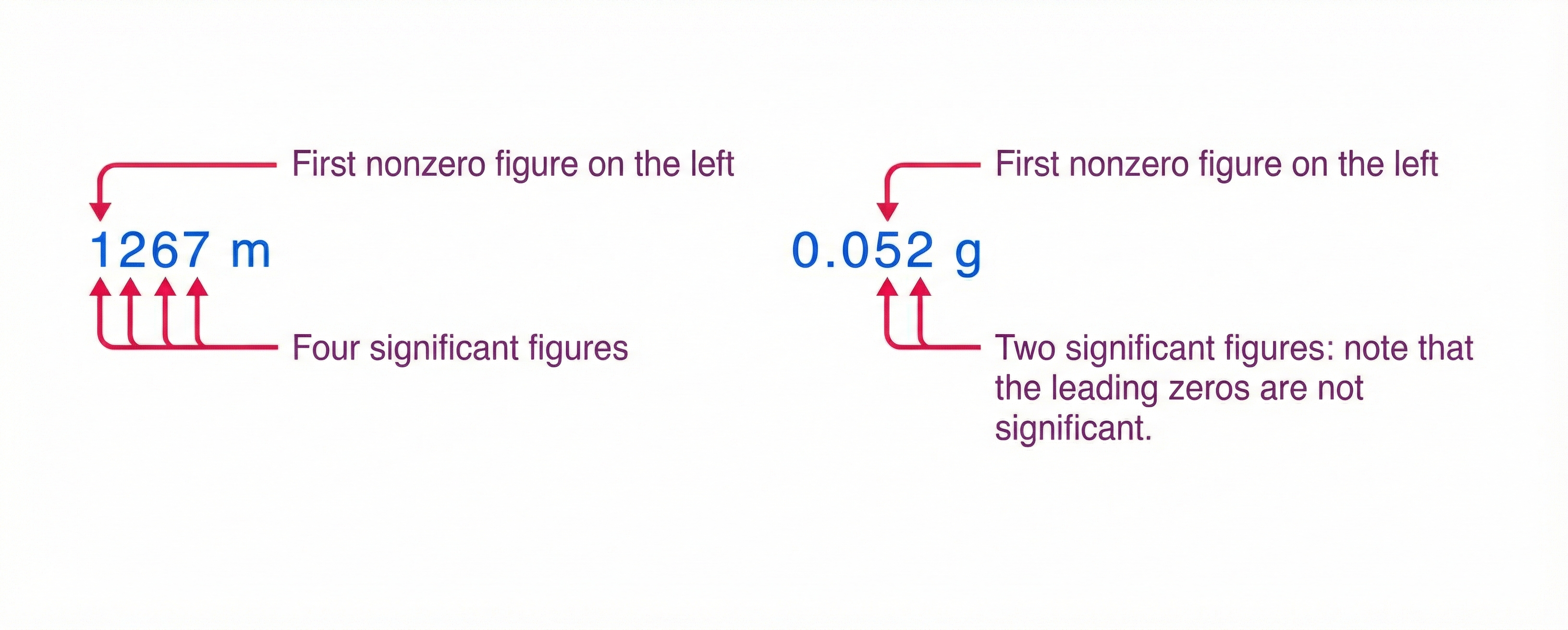
Fig. 1.4 Examples showing how to identify significant figures. The figure was inspired by BYJU’s chemistry.#
1.5.3.1. Zeros#
Special consideration is given to zeros when counting significant figures. The zeros in \(0.052\ {\rm g}\) (see Fig. 1.4) are not significant because they are placeholders that locate the decimal point. The zeros in \(10.053\) are significant because they are bounded (on left and right) by nonzero numbers. The number has five significant figures.
The zeros in \(1300\) may or may not be significant because you can measure exactly that amount or rounded to the nearest significant figure based on your measuring tool. To avoid this ambiguity, we should write \(1300\) in scientific notation as
\(1.3 \times 10^3\) (2 sig figs),
\(1.30 \times 10^3\) (3 sig figs), or
\(1.300 \times 10^3\) (4 sig figs),
depending on the precision of the measurement. Zeros are significant except when they serve only as placeholders.
Checkpoint
Why is \(1300\) ambiguous, but \(1.30 \times 10^3\) is not?
Situation |
Rule |
Example |
|---|---|---|
Multiplication or division |
Match the number of significant figures in the least precise measured value. |
\(10.2\ {\rm m}\) has 3 significant figures, so \(\pi(10.2\ {\rm m})^2\) should be reported with 3 significant figures. |
Addition or subtraction |
Match the least precise decimal place. |
\(7.56\ {\rm kg} - 6.052\ {\rm kg} + 13.7\ {\rm kg}\) is rounded to the tenths place. |
Exact counted values or defined conversion factors |
Do not limit the number of significant figures. |
\(1\ {\rm km} = 1000\ {\rm m}\) is exact. |
Ambiguous trailing zeros |
Use scientific notation to show the intended precision. |
\(1.30 \times 10^3\) has 3 significant figures. |
1.5.3.2. Significant figures in calculations#
When combining measurements with different degrees of precision with arithmetic operations (i.e., addition, subtraction, multiplication, division), then the final number of significant digits can be no greater than the least-precise measured value. There are separate rules for: addition/subtraction and multiplication/division.
For addition and subtraction, the answer can contain no more decimal places than the least precise measurement. For example,
\[ 7.56\ {\rm kg} - 6.052\ {\rm kg} + 13.7\ {\rm kg} = 15.208\ {\rm kg} \approx 15.2\ {\rm kg}, \]where the final value is rounded to the tenths place because the least precise value \(13.7\ {\rm kg}\) is measured to the tenths place.
For multiplication and division, the result should have the same number of significant figures as the least precise measurement. For example,
\[ \pi \times (10.2\ {\rm m})^2 = 326.85129\ldots\ {\rm m^2} \approx 327\ {\rm m^2}, \]where the final value is rounded to the ones place because \(10.2\ {\rm m}\) has 3 significant figures.
1.6. Solving Problems in Physics#
This narration is AI-generated from the course text.
Physics problems are not solved by memorizing formulas. They are solved by building a model, applying mathematics consistently, interpreting the result, and checking the work. Throughout this book, worked examples and exercises follow a common structure to reinforce this process.
1.6.1. The Model (Strategy)#
The first step in solving any physics problem is to decide how to represent the physical situation. This involves identifying the relevant physical quantities, assumptions, and relationships before writing down equations.
A useful strategy is to ask:
What physical quantities are involved?
What is known and what is unknown?
What simplifying assumptions are reasonable?
What definitions, principles, or laws apply?
At this stage, we are not “doing math” yet. We are building a conceptual model of the problem that can later be translated into equations.
1.6.2. The Math (Solution)#
Once a model has been established, the next step is to translate it into mathematics.
This typically involves:
writing equations using symbols rather than numbers,
applying definitions or relationships consistently,
performing algebraic manipulations to isolate the desired quantity,
and substituting numerical values only at the final stage.
As an illustrative example, suppose we wish to convert a speed of \(180\ {\rm km/h}\) into SI units of meters per second.
Using the conversion factors
we write
Keeping units visible throughout the calculation helps prevent mistakes and makes cancellations explicit.
1.6.3. The Conclusion (Significance)#
After obtaining a result, it is essential to interpret it.
A good conclusion addresses questions such as:
Are the final units correct?
Is the numerical value physically reasonable?
Does the result make sense given the original problem?
In the example above, a speed of \(50\ {\rm m/s}\) corresponds to a fast-moving vehicle, which is consistent with an initial speed of \(180\ {\rm km/h}\). The units and magnitude confirm that the result is reasonable.
This step is not optional.
1.6.4. The Verification (Script in Python)#
In this course, Python is often used as a verification tool to confirm analytical work. Code should reflect the same logic used in the mathematics, not replace it.
The following Python script verifies the unit conversion performed above:
# Convert 180 km/h to m/s
velocity_kmh = 180.0

# Conversion factors
km_to_m = 1e3       # meters in a kilometer
h_to_s = 3600.0     # seconds in an hour

# Perform conversion
velocity_ms = velocity_kmh * km_to_m / h_to_s

print(f"Velocity = {velocity_ms:.1f} m/s")
Velocity = 50.0 m/s
1.7. In-class Problems#
What your group notebook should include
For each worked problem, your group should include:
The Model — coordinate system, sign convention, assumptions, and physical interpretation.
The Math — equations introduced by complete sentences, with matching components combined correctly.
The Conclusion — final numerical answer with units and a short physical interpretation.
The Verification — Python confirmation when requested or when useful.
A rough draft is acceptable during class, but the submitted version should be readable enough that another student could follow your reasoning.
Problem 1
(a) Calculate the number of cells in a hummingbird assuming the mass of an average cell is 10 times the mass of a bacterium. See Fig. 1.2.
(b) Making the same assumption, how many cells are there in a human?
Problem 2
The following times are given in seconds. Use metric prefixes to rewrite them so the numerical value is greater than one but less than 1000. For example, \(7.9 \times 10^{-2}\, {\rm s}\) could be written as either 7.9 cs or 79 ms.
(a) \(9.57 \times 10^{5}\,{\rm s}\)
(b) \(0.045\,{\rm s}\)
(c) \(5.5 \times 10^{-7}\,{\rm s}\)
(d) \(3.16 \times 10^{7}\,{\rm s}\)
Problem 3
The following masses are written using metric prefixes on the gram. Rewrite them in scientific notation in terms of the SI base unit of mass: the kilogram. For example, 40 Mg would be written as \(4 \times 10^{4}\,{\rm kg}\).
(a) 23 mg
(b) 320 Tg
(c) 42 ng
(d) 7 g
(e) 9 Pg
Problem 4
American football is played on a 100-yd-long field, excluding the end zones. How long is the field in meters? (Assume that \(1\,{\rm m} = 3.281\,{\rm ft}\).)
Problem 5
Light travels a distance of about \(3 \times 10^{8}\,{\rm m/s}\). A light-minute is the distance light travels in 1 min. If the Sun is \(1.5 \times 10^{11}\,{\rm m}\) from Earth, how far away is it in light-minutes?
Problem 6
Suppose your bathroom scale reads your mass as 65 kg with a 3% uncertainty. What is the uncertainty in your mass (in kilograms)?
Problem 7
(a) If your speedometer has an uncertainty of 2.0 km/h at a speed of 90 km/h, what is the percent uncertainty?
(b) If it has the same percent uncertainty when it reads 60 km/h, what is the range of speeds you could be going?
1.8. Homework#
1.8.1. Conceptual Questions#
Problem 1
What are the SI base units of length, mass, and time? What are the equivalent Imperial units? Compare the two systems of units.
Problem 2
A student proposes the following equation for the position of an object moving along a straight line:
where \(x\) is position, \(v\) is velocity, \(a\) is acceleration, and \(t\) is time.
a. Determine whether this equation is dimensionally consistent.
b. If it is not, identify which term is incorrect and explain why based on units.
1.8.2. Problems#
Problem 3
A car travels at a constant speed of \(72\ {\rm km/h}\).
a. Convert this speed to meters per second.
b. Without performing any calculations, state whether the numerical value of the speed should increase or decrease during this conversion and explain why.
Problem 4
A distance is measured as \(12.4\ {\rm m}\) and the corresponding time interval is measured as \(3.02\ {\rm s}\).
a. Calculate the average speed.
b. Report your result using the correct number of significant figures.
c. Explain how you determined the number of significant figures in the final answer.
Problem 5
Estimate the order of magnitude of the number of seconds in one year.
You may assume:
\(1\ {\rm day} = 24\ {\rm hours}\)
\(1\ {\rm hour} = 3600\ {\rm s}\)
a. Show your reasoning clearly.
b. Express your final answer as a power of ten.
Problem 6
A spacecraft travels a distance of \(3.0 \times 10^8\ {\rm m}\) in a time interval of \(1.5 \times 10^3\ {\rm s}\).
a. Calculate the average speed in meters per second.
b. Convert the distance to kilometers and recompute the average speed in kilometers per second.
c. Briefly explain which unit system is more convenient for this situation and why.