6. Quantum Mechanics: Part II#
6.1. The Schrödinger Wave Equation#
In November 1925, Schrödinger was presenting on de Broglie’s wave theory for particles when Peter Debye suggested that there should be a wave equation. Within a few weeks, Schrödinger found a suitable equation based on what he knew about geometrical and wave optics.
Note
Schrödinger’s equation permits wave-like solutions even though it is not strictly a wave equation in a mathematical sense (see Eqn. (5.8)). It is more analogous to a diffusion equation with a diffusion coefficient \(\beta^2 = h/2m\) (Mita 2021).
Newton’s laws govern the motion of particles, where we need a similar set of equations to describe the wave motion of particles. A wave equation is needed that is dependent on the potential field that the particle experiences. The wave function \(\Psi\) is operated on by the field and allows us to calculate the physical observables (e.g., position, energy, momentum, etc.). Note that we will not be able to determine the exact position and momentum simultaneously due to the uncertainty principle.
The Schrödinger wave equation in its time-dependent form for a particle moving in a potential \(V\) in one dimension is
which is a complex partial differential equation (PDE). Both the potential \(V\) and the wave function \(\Psi\) may be functions of space and time (i.e., \(V(x,t)\) and \(\Psi(x,t)\)). The extension of Eqn. (6.1) into three dimensions is straightforward,
but this introduction is restricted to the one-dimensional form until Section 6.5.
Exercise 6.1
The wave equation must be linear so that we can use the superposition principle to form wave packets comprised of two or more waves. Prove that the wave function in Eqn. (6.1) is linear by using the addition of two waves by using two waves (\(\Psi_1\) and \(\Psi_2\)) with constant coefficients (\(a\) and \(b\)) as
which satisfies the Schrödinger equation.
To apply the Schrödinger equation, we need to know the partial derivatives of \(\Psi\) with respect to time \(t\) and position \(x\). These derivatives are
Substituting these derivatives into Eqn. (6.1) produces
Collecting all the \(\Psi_1\) terms to the left-hand side and the \(\Psi_2\) terms to the right-hand side gives
If \(\Psi_1\) and \(\Psi_2\) satisfy Eqn. (6.1) individually, then the quantities in parentheses are identically zero. Therefore \(\Psi\) is also a solution.
A wave can be characterized by a wave number \(k\) and angular frequency \(\omega\) traveling in the \(+x\) direction by
However, Eqn. (6.2) could be generalized to be a complex function with both sines and cosines. A more general form of a wave function is
where the coefficient \(A\) can be complex. The complex exponential \(e^{i(kx-\omega t)}\) is an acceptable solution to the time-dependent Schrödinger wave equation, but not all functions of \(\sin(kx-\omega t)\) and \(\cos(kx-\omega t)\) are solutions.
Exercise 6.2
(a) Show that \(\Psi_A(x,t) = Ae^{i(kx-\omega t)}\) satisfies the time-dependent Schrödinger wave equation.
(b) Determine whether \(\Psi_B(x,t) = A\sin(kx-\omega t)\) is an acceptable solution to the time-dependent Schrödinger wave equation.
(a) Similar to the previous example, we need to take the appropriate partial derivatives of the wave function \(\Psi_A\) with respect to time as
and with respect to space as
Now we insert the results into Eqn. (6.1) to get
If we use \(E=hf=\hbar \omega\) and \(p = \hbar k\), we obtain
which is zero in our nonrelativistic formulation, because \(E = K + V = p^2/(2m) + V\). Thus \(\Psi_A\) appears to be an acceptable solution.
(b) Similar to part a, we need to take the appropriate partial derivatives of the wave function \(\Psi_B\) with respect to time as
and with respect to space as
Now we insert the results into Eqn. (6.1) to get
The left-hand side of the above result is complex where the right-hand side is real. Therefore, \(\Psi_B\) is not an acceptable wave function because Eqn. (6.1) is not satisfied for all \(x\) and \(t\). The function \(\Psi_B\) is a solution to the classical wave equation.
6.1.1. Normalization and Probability#
The probability \(P(x)\ dx\) of a particle between \(x\) and \(x+dx\) is given as
where the complex conjugate operator \(^*\) negates the complex parts of a function (i.e., \(i\rightarrow -i\)) and leaves the real parts unchanged. The probability of a particle existing between two points (\(x_1\) and \(x_2\)) is given by
If the wave function represents the probability of a particle existing somewhere, then the sum of all probability intervals must equal unity, or
which is called normalization.
Show code cell content
import numpy as np
import matplotlib.pyplot as plt
from myst_nb import glue

def Psi_alpha(x,A):
    #calculate the wave function Ae^{-|x|/alpha}; alpha is a global variable
    #A = normalization constant
    return A*np.exp(-np.abs(x)/alpha)

fs = 'medium'
lw = 2
col = (218/256., 26/256., 50/256.)

alpha = 1. #scale of the plot
norm_A = 1./alpha
x_rng = np.arange(-5*alpha,5*alpha,0.01)
x_a = np.arange(0,1,0.01)
x_b = np.arange(1,2,0.01)

fig = plt.figure(figsize=(6,3),dpi=150)
ax = fig.add_subplot(111)

Psi_all = Psi_alpha(x_rng,norm_A)
Psi_a = Psi_alpha(x_a,norm_A)
Psi_b = Psi_alpha(x_b,norm_A)
ax.plot(x_rng,Psi_all,'-',color=col,lw=lw,label='$\Psi(x) = Ae^{-\\frac{|x|}{\\alpha}}$')
ax.fill_between(x_a,Psi_a,color='gray',alpha=0.5)
ax.fill_between(x_b,Psi_b,color='b',alpha=0.75)
ax.axvline(0,color='k',linestyle='-',lw=lw)
ax.legend(loc='best',fontsize=fs)

ax.set_ylim(0,1.1*norm_A)
ax.set_yticks([0,1])
ax.set_yticklabels(['0','A'])
ax.set_xticks(range(-5,6))
ax.set_xlim(-5,5)
ax.set_xlabel("Position ($\\alpha$)",fontsize=fs)

glue("psi_fig", fig, display=False);

Fig. 6.1 The wave function \(\Psi(x) = Ae^{-\frac{|x|}{\alpha}}\) is plotted as a function of \(x\). The area under the curve represents the probability to find the particle between \(x_1\) and \(x_2\). Note that the wave function is symmetric about \(x=0\).#
Exercise 6.3
Consider a wave packet formed by using the wave function \(\Psi(x) = Ae^{-\frac{|x|}{\alpha}}\), where \(A\) is a constant to be determined by normalization (Fig. 6.1). Normalize this wave function and find the probabilities of the particle being between (a) \(0\) and \(\alpha\) (gray area in Fig. 6.1 ) and (b) \(\alpha\) and \(2\alpha\) (blue area in Fig. 6.1).
To normalize the wave function \(\Psi\), we use Eqn. (6.4) by
Because the wave function is symmetric about \(x=0\), we can evaluate only the positive interval \((0\leq x \leq \infty\)), multiply by \(2\), and drop the absolute value signs on \(|x|\) to get
The coefficient \(A = \alpha^{-1/2}\), and the normalized wave function \(\Psi\) is
We use the above result to determine the probability of the particle existing within each interval. Since the intervals are on the positive \(x\)-axis, we drop the absolute value signs on \(|x|\) to get
The probability in the other interval is
The particle is much more likely to exist in interval (a) than in interval (b). This is expected given the shape of the wave function.
The wave function \(e^{i(kx-\omega t)}\) represents a “free” particle under zero net force (constant \(V\)) moving along the \(x\) axis. There is a problem with this wave function if we try to normalize it. The normalization integral diverges to infinity!
This occurs because there is a finite probability of the particle to exist anywhere along the \(x\) axis and our sum is trying to add up an infinite number of small boxes containing a finite probability. The only other possibility is a zero probability, but that is not an interesting physical result.
Because this wave function has a precise \(k\) and \(\omega\), it represents a particle with a definite energy and momentum. From the uncertainty principle, \(\Delta E = 0\) and \(\Delta p = 0\), which implies that \(\Delta t = \infty\) and \(\Delta x = \infty\). We cannot know where the particle is at any time. We can still use such wave functions, if we restrict the particle to certain positions in space, such as in a box or in an atom. We can also form wave packets from such functions to localize the particle.
6.1.2. Properties of Valid Wave Functions#
There are certain properties (i.e., boundary conditions) that an acceptable wave function \(\Psi\) must:
be finite everywhere to avoid infinite probabilities.
be single valued to avoid multiple values of the probability.
be continuous for finite potentials. Its spatial derivative \(\partial \Psi/\partial x\) must also be continuous. This is required due to the second-order derivative term in the Schrödinger equation. (There are exceptions to this rule for infinite potentials).
must approach zero as \(x \rightarrow \pm \infty\) to normalize the wave functions.
Solutions for \(\Psi\) that do not satisfy these properties do not generally correspond to physically realizable circumstances.
6.1.3. Time-Independent Schrödinger Wave Equation#
In many cases, the potential will not depend explicitly on time (i.e., time-independent). The dependence on time and position can then be separated in the Schödinger equation. Let \(\Psi(x,t) = \psi(x)f(t)\), and insert into Eqn. (6.1) to find
Dividing by \(\psi(x) f(t)\), we get
Notice that the left-hand side depends only on time, while the right-hand side depends only on spatial coordinates. This allows us to change the partial derivatives to ordinary derivatives because each side depends only on one variable. Each side must be equal to a constant because one variable may change independently of the other. Let’s call this constant \(B\) and set it equal to the left-hand side to get
We can integrate both sides and find
which includes the integration constant \(C\) that we may choose to be 0. Then,
and we determine \(f\) to be
If we let \(B = \hbar \omega = E\), then \(f(t) = e^{-i\omega t} = e^{-\frac{iEt}{\hbar}}\). We can now write the time-independent Schödinger equation as
The wave function \(\Psi(x,t)\) becomes
Many important results can be obtained when only the spatial part of the wave function \(\psi(x)\) is needed.
The probability density used the complex conjugate operator, which now becomes useful. Using Eqn. (6.7), we have
where the probability distributions are constant in time. If the probability distribution represents a wave, then we have the phenomenon of standing waves. In quantum mechanics, we say the system is in a stationary state.
Exercise 6.4
Consider a metal in which there are free electrons, and the potential is zero (e.g., a conductor). What mathematical form does the wave function \(\psi(x)\) take?
Using Eqn. (6.7), we let \(V(x)=0\) to get
and using Eqn. (5.35), we find
The differential equation \(d^2\psi/dx^2 = -k^2\psi\) has appeared several times in calculus and introductory physics (e.g., pendulum and simple harmonic motion).
If the energy \(E>0\), then \(k^2\) is real and the wave function solution is
Otherwise (\(E<0\)), then \(k^2\) is imaginary and the wave function solution is
6.1.4. Comparison of Classical and Quantum Mechanics#
Newton’s second law (\(\vec{F} = m\vec{a}\)) and Schrödinger’s equation are both differential equations that are postulated to explain observed behavior, and experiments show that they are successful. Newton’s second law can be derived from the Schrödinger equation. Schrödinger’s equation is more fundamental. Classical mechanics only appears to be more precise because it deals with macroscopic phenomena, where the underlying uncertainties are just too small to be significant.
An interesting parallel between classical and quantum mechanics lies in considering ray and wave optics. Throughout the 18th century, scientists argued whether wave or ray optics was more fundamental (Newton favored ray optics). In the early 19th century, it was shown that wave optics was need to explain diffraction and interference. Ray optics is a good approximation as long as the wavelength \(\lambda\) is much smaller than the dimensions of the apertures because rays of light are characteristic of particle-like behavior. To describe interference phenomena, wave optics is required.
For macroscopic objects, the de Broglie wavelength is so small that wave behavior is not apparent. Eventually the wave descriptions and quantum mechanics were required to understand all the data. Classical mechanics is a good macroscopic approximation, but there is only one correct theory, quantum mechanics, as far as we know.
6.2. Expectation Values#
The wave equation formalism must measure physical quantities (e.g., position, momentum, and energy). Consider a measurement of the the position \(x\) of a particular system. If we make three measurements of the position, we are likely to obtain three different results due to uncertainty. If our method of measurement is inherently accurate, then there is some physical significance to the average of our measure values of \(x\).
The precision of our result improves with additional measurement. In quantum mechanics, we use wave functions to calculate the expected result of the average of many measurements of a given quantity. Measurements are made through integration, which returns the average value (recall the mean value theorem from calculus). We call this result the expectation value, where the expectation value of \(x\) is \(\langle x \rangle\). *Physical observables are found the the epxectation value. The expectation value mus be real (i.e., not complex) because the results of measurements are real.
Consider a particle that is constrained to move along the \(x\)-axis. If we make many measurements of the particle, we may observe the particle at the position \(x_1\) for a number \(N_1\) times, the position \(x_2\) for \(N_2\) times, and so forth. The average value of \(x\) (i.e., \(\bar{x}\) or \(x_{\rm av}\)) is then
from a series of discrete measurements. For continuous variables, we use the probability \(P(x,t)\) of observing the particle at a particular \(x\). Then the average value of \(x\) is
In quantum mechanics, we use the probability distribution (i.e., \(P(x)dx = \Psi^*(x,t)\Psi(x,t) dx\)) to determine the average or expectation value. The expectation value \(\langle x \rangle\) is given by
The denominator is the normalization equation. If the wave function is normalized, then the denominator is equal to unity. For a normalized wave function \(\Psi\), the expectation value is then given by
The same general procedure is applicable to determining the expectation value of any function \(g(x)\) for a normalized wave function \(\Psi(x,t)\) by
Any knowledge we might have of the simultaneous value of the position \(x\) and the momentum \(p\) must be consistent with the uncertainty principle. To find the expectation value of \(p\), we need to represent \(p\) in terms of \(x\) and \(t\). Consider the wave function of the free particle, \(\Psi(x,t) = e^{i(kx-\omega t)}\). The spatial derivative is
Since \(k = p/\hbar\), this becomes
or
An operator is a mathematical operation that transforms one function into another. Coffee is the operator that transforms ideas into knowledge! An operator, denoted by \(\hat{Q}\), transforms the function \(f(x)\) by \(\hat{Q}f(x) = g(x)\). The momentum operator \(\hat{p}\) is then represented by
where the \(\hat{\ }\) symbol (i.e., “hat”) sign over the letter indicates that it is an operator.
The momentum operator is not unique, where each of the physical observables has an associated operator that used to find the observable’s expectation value. To compute the expectation value of some physical observable \(Q\), the operator \(\hat{Q}\) must operate on \(\Psi\) before calculating the probability to get
The expectation value of the momentum \(p\) becomes
The position \(x\) is its own operator (i.e., \(\hat{x} = x\)). Operators for observables of both \(x\) and \(p\) can be constructed from \(\hat{x}\) and \(\hat{p}\).
The energy operator \(\hat{E}\) can be constructed from the time derivative of the free-particle wave function,
Substituting \(\omega = E/\hbar\) and rearranging, we find
The energy operator \(\hat{E}\) is used to find the expectation value \(\langle E \rangle\) of the energy by
The application of operators are general results and not limited to just free-particle wave functions.
Exercise 6.5
Use the momentum and energy operators with the conservation of energy to produce the Schrödinger wave equation.
The conservation of energy tells us how to calculate the total energy
We replace \(p\) with the operator and apply to the wave function \(\Psi\), which gives
Notice that \(\hat{p}^2\) results in applying \(\hat{p}\) twice. Using the application of the energy operator from Eqn. (6.17), we obtain
which is the time-dependent Schrödinger wave equation. This is not a derivation, but only a verification of the consistency of the definition.
6.3. Infinite Square-Well Potential#
The simplest system consists of a particle trapped in a well with infinitely hard walls that the particle cannot penetrate (i.e., particle-in-a-box). This scenario was explored in Sect. 5.8, but now we present the full quantum mechanical solution.
The potential that gives rise to an infinite square well with a width \(L\) is given by
The particle is constrained to move only between \(x=0\) and \(x=L\), where the particle experiences no forces. The infinite square-well potential can approximate many physical situations, such as the energy levels of simple atomic and nuclear systems.
If we insert the infinite square-well potential into the the time-independent Schödinger equation (Eqn. (6.7)),
the only possible solution for the region \(x=\leq 0\) or \(x\geq L\) is the wave function \(\psi(x) = 0\) because \(V = \infty\). There is zero probability for the particle to exist in this region.
the region \(0<x<L\) permits a nonzero solution because \(V=0\). The probability for the particle to exist in this region is 1.
Using \(V=0\) in Eqn. Eqn. (6.7) produces
where the wave number \(k = \sqrt{2mE/\hbar^2}\). A suitable solution to this equation is
where \(A\) and \(B\) are constants used to normalize the wave function. The wave function must be continuous at the boundaries, which means that \(\psi(0)=\psi(L) = 0\). Let’s apply these boundary conditions as
For \(\psi(0) = 0\), this implies that \(B=0\). To apply \(\psi(L) = 0\), then \(A\sin(kL) = 0\) and \(A=0\) is a trivial solution. We must have
for \(\sin(kL) = 0\) and \(n\) is a positive integer. The wave function is now
The property that \(d\psi /dx\) must also be continuous so that we can normalize the wave function. The normalization condition is
where substitution of the wave function yields
This is a straightforward integral (with the help of an integral table) and gives \(L/2\), so that \(A^2(L/2) = 1\) and \(A = \sqrt{2/L}\). The normalized wave function becomes
These wave functions are identical to a vibrating string with its ends fixed. The application of the boundary conditions corresponds to fitting standing waves into the box. It is not a surprise to find standing waves as the solution because wea are considering time-independent solutions. Since \(k_n = n\pi/L\), we have
Notice the subscript \(n\) that denotes quantities that depend on the integer \(n\) and have multiple values. This equation is solved for \(E_n\) to give
The possible energies \(E_n\) of the particle are quantized and the integer \(n\) is a quantum number. The quantization of energy occurs from the application of the boundary conditions (standing waves) to possible solutions of the wave equation. Each wave function \(\psi_n(x)\) has associated with it a unique energy \(E_n\). The lowest energy level given by \(n=1\) is called the ground state and has an energy \(E_1 = \pi^2\hbar^2/(2mL^2)\).
Note that the lowest energy level cannot be zero because the wave function has zero probability (\(\psi_0 = 0\)). Classically the particle has equal probability of being anywhere inside the box. The classical probability density is \(P(x) = 1/L\). According to Bohr’s correspondence principle, we should obtain the same probability for large \(n\), where the classical and quantum results should agree. The quantum probability density is \((2/L)\sin^2(k_n x)\).
For large values of \(n\), there will be many oscillations within the box and the average value of \(\sin^2 \theta\) over many cycles is \(1/2\). Therefore the quantum probability for large \(n\) is equal to \(1/L\), in agreement with the classical result.
Useful Integrals
Exercise 6.6
Determine the expectation values for (a) \(x\), (b) \(x^2\), (c) \(p\), and (d) \(p^2\) of a particle in an infinite square well for the first excited state.
The first excited state corresponds to \(n=2\), and we know the quantized (normalized) wave function for a particle in an infinite square well from Eqn. (6.24). This gives
(a) Using \(\psi_2(x)\), we can find the expectation value of \(x\) through the integral (using an integral table)
The average position of the particle is in the middle of the box \((x=L/2)\), although this is not the most probable location.
(b) The expectation value of \(x^2\) is found through
where you can use integration by parts, an integral table, or the python module sympy. the expectation value for \(\sqrt{\langle x^2\rangle}\) for the first excited state is \(0.57L\), which is larger than \(\langle x \rangle\).
(c) The expectation value of \(p\) requires the first derivative \(d\psi_2/dx\), which is,
Applying this result to the integral for \(\langle p \rangle\) gives,
The integral of \(\sin x \cos x\) over symmetric limits is always zero because the particle is moving left as often as right in the box.
(d) The expectation value for \(p^2\) requires us to operate a second time on \(\psi_2\) to get
Applying this result to the integral for \(\langle p^2 \rangle\) gives,
Using \(\langle p^2\rangle\), we can calculate the energy of the first excited state as
which is correct because \(V=0\).
from sympy import symbols, pi, simplify, integrate, diff, sin, var

var('x')
i, hbar, L = symbols('i, hbar L')
psi = sin(2*pi*x/L)

#find integral for <x>
exp_x = simplify(integrate((2/L)*x*psi**2,(x,0,L)))
print("The expectation value for x is",exp_x)

#find integral for <x^2>
exp_x2 = simplify(integrate((2/L)*(x*psi)**2,(x,0,L)))
print("The expectation value for x**2 is", exp_x2, '= [1/3 - 1/(8*pi**2)]*L**2 = %1.2f L**2' % (1/3 - 1/(8*pi**2)))

#find integral for <p>
exp_p = simplify(integrate((2/L)*psi*diff(i*hbar*psi,x),(x,0,L)))
print("The expectation value for p is", exp_p)

#find integral for <p^2>
exp_p2 = simplify(integrate((2/L)*psi*diff(diff(-hbar**2*psi,x),x),(x,0,L)))
print("The expectation value for p**2 is", exp_p2.args[0][0])
The expectation value for x is L/2
The expectation value for x**2 is -L**2/(8*pi**2) + L**2/3 = [1/3 - 1/(8*pi**2)]*L**2 = 0.32 L**2
The expectation value for p is 0
The expectation value for p**2 is 4*pi**2*hbar**2/L**2
6.4. Finite Square-Well Potential#
An infinite potential well is not very realistic. The finite-well potential is more realistic and similar to the infinite one. Consider a potential that is zero between \(x=0\) and \(x=L\), but equal to a constant \(V_o\) everywhere else. This is written mathematically as
First, let’s examine a particle of energy \(E < V_o\) that is classically bound inside the well. Using Eqn. (6.7), we have
Let \(\alpha^2 = 2m(V_o-E)/\hbar^2\) (a positive constant), and we find
The solution to this differential equation is known and can be written as a combination of exponential functions (\(e^{\alpha x}\) and \(e^{-\alpha x}\)), or
A valid wave function needs to be finite everywhere, where we can use this constraint to determine the form of the wave function \(\psi\) within region I and region III. Region I includes all values of \(x\leq -L\), where we can try to evaluate what conditions are necessary for \(\psi\) to be finite using a limit,
which requires that \(B = 0\). Similarly, we can use a limit to find that \(A=0\) for \(x\geq L\). This allows us to define the wave functions in each region as
Inside the square well, the potential is zero and the Schrödinger equation becomes
where \(k=\sqrt{(2mE)/\hbar^2}\). This differential equation has a solution, which is a combination of sinusoidal functions:
To determine a valid wave function, it must be continuous at the boundary (e.g., \((\psi_I = \psi_{II})\) and \((d\psi_I/dx = d\psi_{II}/dx)\) at \(x=-L\)). By choosing symmetric boundaries and noting that the potential is an even function (i.e., \(V_ox^0\)), we can simplify \(\psi_{II}\) to include only the even portion (i.e., \(D=0\)). As a result, we find the following conditions
We immediately find that \(B=A\), and we can divide the last two equations to eliminate \(C\) to get,
Recall that \(k\) and \(\alpha\) are both functions of energy \(E\). To solve for \(E\), we perform a variable transformation \(z \equiv kL\) and \(z_o \equiv \frac{L}{\hbar}\sqrt{2mV_o}\). Using the definitions of \(k\) and \(\alpha\), we find that
Combining the factors of \(z\) produces,
Completing the transformation, we get
We are left with a transcendental equation that must be solved numerically, where the equation depends on \(z_o\) (i.e., the size of the well) and \(z\) (i.e., a measure of the energy because \(k\propto \sqrt{E}\)). The wave functions can be determined through normalization (more details here).
Show code cell content
import numpy as np
import matplotlib.pyplot as plt
from scipy.optimize import newton
from myst_nb import glue

def fsw(z):
    #Calculate the root for the finite square well (symmetric case)
    return np.tan(z) - np.sqrt((z_o/z)**2-1)
def fsw_prime(z):
    #Calculate the derivative of fsw
    return 1./np.cos(z)**2 + z_o/np.sqrt((z_o/z)**2-1)/z**3

fs = 'medium'
lw = 1.5
col = (218/256., 26/256., 50/256.)

z = np.arange(0.01,3*np.pi,0.01)
z_o = 8 #Example from Griffiths (Fig. 2.13)
z1 = np.arange(0,np.pi/2,0.01)

fig = plt.figure(figsize=(4,2),dpi=300)
ax = fig.add_subplot(111)

for i in range(0,3):
    z1 = np.arange(i*np.pi,(2*i+1)*np.pi/2,0.01)
    if i == 0:
        ax.plot(z1,np.tan(z1),'-',color=col,lw=lw,label='$\\tan(z)$')
    else:
        ax.plot(z1,np.tan(z1),'-',color=col,lw=lw)
ax.plot(z[z<z_o],np.sqrt((z_o/z[z<z_o])**2-1),'k-',lw=lw,label='$\sqrt{(z_o/z)^2-1}$')
ax.legend(bbox_to_anchor=(-0.05, 1.05, 1., .102),ncol=2,fontsize=fs,frameon=False)

roots = []
for i in range(0,3):
    z_guess = 1.4 + i*np.pi
    z_root = newton(fsw,z_guess,fsw_prime)
    ax.plot(z_root,np.tan(z_root),'b.',ms=8)
    roots.append(z_root)

#print("The first three roots are approximately %1.2f pi, %1.2f pi, and %1.2f pi." % (roots[0]/np.pi,roots[1]/np.pi,roots[2]/np.pi))

ax.set_xticks([0,np.pi/2,np.pi,1.5*np.pi,2*np.pi,2.5*np.pi])
ax.set_xticklabels(['0','$\pi/2$','$\pi$','$3\pi/2$','$2\pi$','$5\pi/2$'])
ax.set_xlim(0,3*np.pi)

ax.set_ylim(0,10)
ax.set_yticks([])
ax.set_xlabel("$z$",fontsize=fs)

glue("fsw_fig", fig, display=False);

Fig. 6.2 Graphical solution for the finite square well potential using Eqn. (6.32), for \(z_o = 8\) (even states). The three roots (blue dots) are \(0.44\pi\), \(1.33\pi\), and \(2.17\pi\).#
Show code cell content
import numpy as np
import matplotlib.pyplot as plt
from scipy.constants import m_e, hbar, eV
from scipy.optimize import minimize
from myst_nb import glue

def fsw_wave_func(x,A,C,D,E,V_o,m):
    #Calculate the wave function for the finite square well
    k = calc_k(E,m)
    alpha = calc_alpha(E,V_o,m)
    region_I = np.where(x<=-L)[0]
    region_II = np.where(np.logical_and(-L<x,x<L))[0]
    region_III = np.where(x>=L)

    psi = np.zeros(len(x))
    psi[region_I] = A*np.exp(alpha*x[region_I])
    psi[region_II] = C*np.cos(k*x[region_II])+D*np.sin(k*x[region_II])
    psi[region_III] = A*np.exp(-alpha*x[region_III])

    return psi

def calc_alpha(E,V_o,m):
    #calculate alpha from E and V_o
    return np.sqrt(2*m*np.abs(E-V_o)/hbar**2)
def calc_k(E,m):
    #calculate k from E
    return np.sqrt(2*m*E/hbar**2)

def calc_En(n,m,V_o):
    #calculate E_n for a wide deep well
    #return n**2*np.pi**2*hbar**2/(2*m*(2*L)**2) - V_o
    z_n = [0.44*np.pi,1.33*np.pi,2.17*np.pi]
    return z_n[n]**2*hbar**2/(2*m*L**2)
def calc_coeff(E,V_o,m):
    #calculate the coefficient A_n
    k = calc_k(E,m)
    alpha = calc_alpha(E,V_o,m)
    term_1 = (np.exp(2*alpha*L)-np.exp(-2*alpha*L))/(2*alpha)
    term_2 = (L + np.sin(2*k*L)/(2*L))*np.exp(-2*alpha*L)/np.cos(k*L)**2
    A_n = np.sqrt(1./(term_1+term_2))
    C_n = A_n*np.exp(-alpha*L)/np.cos(k*L)
    return A_n, C_n

fs='medium'
lw = 2
col = (218/256., 26/256., 50/256.)

L = 5.29e-11 #half-width of well (in m)
V_pot = (8*hbar/L)**2/(2*m_e) #z_o = 8 converted into V_o
E_n = []
for i in range(1,4):
    E_n.append(calc_En(i-1,m_e,V_pot))
fig = plt.figure(figsize=(4,4),dpi=150)
ax = fig.add_subplot(111)

x_rng = np.arange(-2*L,2*L,L/40.)
for i in range(0,3):
    A_n,C_n = calc_coeff(E_n[i],V_pot,m_e)
    psi = fsw_wave_func(x_rng,A_n,C_n,0,E_n[i],V_pot,m_e)/1e-5
    ax.fill_between(x_rng[x_rng<=-L]/L,psi[x_rng<=-L]+3.5*i,3.5*i,color='gray')
    ax.fill_between(x_rng[x_rng>=L]/L,psi[x_rng>=L]+3.5*i,3.5*i,color='gray')
    ax.axhline(3.5*i,linestyle='--',color='k')
    ax.plot(x_rng/L,psi+3.5*i,'-',color=col,lw=lw)

ax.set_yticks([])
ax.set_ylim(0,9)
ax.axvline(-1,linestyle='-',color='k')
ax.axvline(1,linestyle='-',color='k')
ax.set_xlim(-2,2)
ax.set_xlabel("$x$ (L)")

glue("fsw_func_fig", fig, display=False);

Fig. 6.3 Wave functions (red curves) for the finite square well using \(z_o = 8\). The gray regions mark where the wave function penetrate into the walls of the potential well.#
The application of the boundary conditions leads to quantized energy values \(E_n\) and associated wave functions \(\psi_n\). Remarkably, the particle has a finite probability of being outside the square well (see Fig. 6.3). Notice that the wave functions joint smoothly at the edges of the well and approach zero exponentially outside the well.
The particle existing outside the well is prohibited classically, but occurs in quantum mechanics. Because of the exponential decrease of the the wave functions (\(\psi_I\) and \(\psi_{III}\)), the probability of the particle penetrating a distance greater than \(\delta x \approx 1/\alpha\) decreases quickly, where
is called the penetration depth. The fraction of particles that successfully tunnel through the outer walls of the potential well is exceedingly small, but the results have important applications.
6.5. Three-Dimensional Infinite-Potential Well#
Like the one-dimensional infinite-potential well, the three-dimensional potential well is expected to have time-independent solutions that can be determined from the time-independent Schrödinger equation. The wave function must depend on all three spatial coordinates, \(\psi =\psi(x,y,z)\). Beginning with the conservation of energy, we multiply by the wave function to get
Then, we use the momentum operator for each dimension because \(\hat{p}^2 = \hat{p}_x^2 + \hat{p}_y^2 + \hat{p}_z^2\). Individually we have
The application of the \(\hat{p}^2\) operator gives
which defines the time-independent Schrödinger equation in three dimensions. The expression in parentheses is the Laplacian operator, which is usually written using the shorthand notation as
and we can write Eqn. (6.35) as
Exercise 6.7
Consider a free particle inside a box with lengths \(L_1\), \(L_2\), and \(L_3\) along the \(x\), \(y\), and \(z\) axes, respectively. The particle is constrained to be inside the box. (a) Find the wave functions and energies. (b) Find the ground-state wave function for a cube. (c) Find the energies of the ground and first excited state for a cube of sides \(L\).
(a) Similar to the one-dimensional infinite square well, it is reasonable to try a sinusoidal wave function for each of the dimensions. As a result, we obtain
which has a normalization constant \(A\) and the quantities \(k_i\) (\(k_1\), \(k_2\), and \(k_3\)) are determined by applying the appropriate boundary conditions.
The condition that \(\psi = 0\) at \(x=L_1\) requires that \(k_1L_1 = n_1\pi\). Generalizing this constraint and solving for \(k_i\), we get
using the integers \(n_1\), \(n_2\), and \(n_3\) for quantum numbers in each of the dimensions.
Now, we need to take the appropriate derivatives of \(\psi\) with respect to \(x\) (the derivatives in \(y\) and \(z\) will be similar). We have
Equation (6.35) becomes
The \(k_i\) represent a wave number for each dimension, where we can generalize the energies of the one-dimensional case to
where the allowed energies depend on the three quantum numbers. The wave function can also be written in terms of the quantum numbers as
(b) For a cube \(L_1 = L_2 = L_3 = L\) and the ground state is given by \(n_1 = n_2 = n_3 = 1\). The ground-state wave function is simply
(c) For a cube the energies are given as
and the ground state energy is \(E_{111} = \frac{3\pi^2\hbar^2}{2mL^2}\).
The first excited state is when one quantum number is increased by one so that
There are three possible combinations for the first excited state depending on which dimension of the cube is excited.
A given state is degenerate when there is more than one wave function for a given energy (see Exercise 6.7). Degeneracies are often the result of symmetries. For a cube, there is a degeneracy, but it is removed if the sides have different lengths because there would be different energies. Degeneracy also occurs in classical physics where orbits with different eccentricities may have the same energy. A perturbation of the potential energy can remove a degeneracy. Energy levels can split (thereby removing a degeneracy) by applying an external magnetic (Zeeman effect) or electric (Stark effect) field.
6.6. Simple Harmonic Oscillator#
Simple harmonic oscillators (SHOs) commonly occur in nature and are one of the first physical systems studied within introductory physics. Consider a spring with a spring constant \(\kappa\), which is in equilibrium at \(x=x_o\). There is a restoring force described through Hooke’s law and a potential energy, which is given as
The application of the restoring force introduces simple harmonic motion (SHM). Diatomic molecules or a system of atoms in a solid lattice can be approximated by SHM in a general way. Within a lattice, the force on the atoms depends on the distance \(x\) from some equilibrium position and the potential \(V(x)\) can be represented by a Taylor series as
where each term of the series has a constant \(V_i\). For \(x-x_o \approx 0\) (i.e., a small perturbation), the higher terms are negligible. The minimum of the potential occurs at the equilibrium position, which means that \(dV/dx = 0\) and the lowest surviving term of the potential is
To study the quantum description of SHM, we insert a potential \(V = kx^2/2\) into Eqn. (6.7) to get
Through a pair of variable transformations,
we get
The particle is confined to the potential well, and thus, has zero probability of being at \(x= \pm \infty\), which means
Additionally, the lowest energy state cannot be \(E=0\) because if \(x=0\) and \(v=0\), then the kinetic energy is also zero (i.e., \(p=0\)). The uncertainty principle prevents us from knowing \(x\) and \(p\) exactly, which means at \(x=0\) that \(p>0\) (i.e., \(E>0\)).
The lowest energy state is defined as some non-zero potential or \(E_o = V_o\). If we represent the energy by a height above the bottom of the well (i.e., some inherent potential energy), then there will be a symmetric distance \(\pm a\) from the equilibrium position to denote the lowest energy (i.e., \(E_o = \kappa a^2/2\)). The walls of the potential are similar to the finite potential well, where there is some small probability of the wave function existing outside the potential. But the wave function decreases rapidly on the other side of the barrier. The minimum energy \(E_o\) is also called the zero-point energy (see Fig. 6.4).
Show code cell content
import numpy as np
import matplotlib.pyplot as plt
from scipy.special import hermite
from scipy.constants import m_e
from myst_nb import glue
from matplotlib import rcParams

rcParams.update({'font.size': 16})
rcParams.update({'mathtext.fontset': 'cm'})

def SHO_potential(x):
    #calculate the SHO potential
    return 0.5*kappa*x**2

def SHO_wave_func(n,x):
    #calculate the SHO wave function
    A = (alpha/np.pi)**0.25
    if n == 0:
        return A*np.exp(-alpha*x**2/2)

alpha  = 1. #Assume alpha = 1 --> kappa = hbar^2/m
kappa = hbar**2*alpha**2/m_e
omega = np.sqrt(kappa/m_e)
a = np.sqrt(hbar*omega/kappa) #width of the potential at E_o

fs = 'medium'
lw = 2
col = (218/256., 26/256., 50/256.)

fig = plt.figure(figsize=(8,4),dpi=150)
ax1 = fig.add_subplot(121)
ax2 = fig.add_subplot(122)

x = np.arange(-3*a,3*a,a/40.)
ax1.plot(x/a,SHO_potential(x)/(hbar*omega),'-',color=col,lw=lw,label='$V(x)$')
ax1.axhline(0.5,0.25,0.75,linestyle='--',lw=1.5)
ax1.axvline(-1,0,0.25,linestyle='--',lw=1.5)
ax1.axvline(1,0,0.25,linestyle='--',lw=1.5)
ax1.axvline(0,0,0.8,linestyle='-',color='k',lw=1.5)
ax1.legend(loc='best',fontsize=fs)

ax2.plot(x/a,SHO_wave_func(0,x),'-',color=col,lw=lw,label='$\psi_o$')
ax2.axvline(-1,0,0.45,linestyle='--',lw=1.5)
ax2.axvline(1,0,0.45,linestyle='--',lw=1.5)
ax2.legend(loc='best',fontsize=fs)

ax1.set_ylim(0,2)
ax1.set_xlim(-2,2)
ax1.set_xlabel("Position $x$ ($a$)",fontsize=fs)
ax1.set_yticks([])

ax2.set_ylim(0,1.)
ax2.set_xlim(-3,3)
ax2.set_xlabel("Position $x$ ($a$)",fontsize=fs)
ax2.set_xticks(range(-2,3))
ax2.set_yticks([])

glue("SHO_fig", fig, display=False);

Fig. 6.4 Simple harmonic oscillator potential (left) and ground state wave function (right). The horizontal (dashed) line represents the zero-point energy.#
Exercise 6.8
Estimate the minimum energy of the simple harmonic oscillator (SHO) allowed by the uncertainty principle.
From classical mechanics, the average kinetic energy is equal to the average potential energy (i.e., \(K_{\rm av}=V_{\rm av}\); virial theorem. As a result, the average potential and kinetic energy are equal to half of the total energy. We can write this mathematically as
Applying this to the SHO gives
The mean value of \(x=0\), but the mean value of \((x^2)_{\rm av} \) is the mean square deviation \((\Delta x)^2\) (see the uncertainty principle in general). A similar reasoning can be applied to get \((p^2)_{\rm av} = (\Delta p)^2\). Then, we must have
From Heisenberg’s uncertainty principle, we have \(\Delta p \Delta x \geq \hbar/2\). Then the minimum value of \(\Delta x = \hbar/(2\Delta p)\). Combining with the previous result, we have
Then, the lowest energy is
The zero point energy for the SHO is \(\frac{1}{2}\hbar \omega\).
Deriving the wave function solutions for the SHO is beyond the our scope. They are written in terms of Hermite polynomial functions \(H_n(x)\) that have an order \(n\) and \(n\) is a positive integer. The wave function general solution and first four \(\psi_n\) are

Fig. 6.5 Simple harmonic oscillator wave functions (left) and probability density functions (right). The vertical (dashed) line represents the with of the potential well at a given energy \(E_n\).#
Show code cell content
import numpy as np
import matplotlib.pyplot as plt
from scipy.special import hermite
from scipy.constants import m_e
from myst_nb import glue
from matplotlib import rcParams

rcParams.update({'font.size': 16})
rcParams.update({'mathtext.fontset': 'cm'})

def SHO_potential(x):
    #calculate the SHO potential
    return 0.5*kappa*x**2

def SHO_wave_func(n,x):
    #calculate the SHO wave function
    psi_o = (alpha/np.pi)**0.25*np.exp(-alpha*x**2/2)
    if n == 0:
        return psi_o
    elif n == 1:
        return np.sqrt(2*alpha)*x*psi_o
    elif n == 2:
        return (2*alpha*x**2-1)/np.sqrt(2)*psi_o
    elif n == 3:
        return np.sqrt(alpha)*x*(2*alpha*x**2-3)/np.sqrt(3)*psi_o

alpha  = 1. #Assume alpha = 10 --> kappa = hbar^2/m
kappa = hbar**2*alpha**2/m_e
omega = np.sqrt(kappa/m_e)
a = np.sqrt(hbar*omega/kappa) #width of the potential at E_o

fs = 'medium'
lw = 2
col = (218/256., 26/256., 50/256.)

fig = plt.figure(figsize=(8,8),dpi=150)
ax11 = fig.add_subplot(421)
ax12 = fig.add_subplot(422)
ax21 = fig.add_subplot(423)
ax22 = fig.add_subplot(424)
ax31 = fig.add_subplot(425)
ax32 = fig.add_subplot(426)
ax41 = fig.add_subplot(427)
ax42 = fig.add_subplot(428)
ax_psi = [ax41,ax31,ax21,ax11]
ax_prob = [ax42,ax32,ax22,ax12]

x = np.arange(-5*a,5*a,a/40.)

for i in range(0,4):
    ax_psi[i].plot(x/a,SHO_wave_func(i,x),'-',color=col,lw=lw,label='$\psi_%i$' % i)
    ax_prob[i].plot(x/a,SHO_wave_func(i,x)**2,'-',color=col,lw=lw,label='$|\psi_%i|^2$' % i)

    x_a = np.sqrt(2*i+1)
    ax_psi[i].axvline(-x_a,linestyle='--',lw=1.5)
    ax_prob[i].axvline(-x_a,linestyle='--',lw=1.5)
    ax_psi[i].axvline(x_a,linestyle='--',lw=1.5)
    ax_prob[i].axvline(x_a,linestyle='--',lw=1.5)

    ax_psi[i].set_yticks([])
    ax_prob[i].set_yticks([])
    ax_psi[i].set_ylim(-1,1)
    ax_prob[i].set_ylim(0,0.45)
    if i == 0:
        ax_psi[i].set_ylim(0,1)
        ax_prob[i].set_ylim(0,0.7)

    ax_psi[i].set_xlim(-5,5)
    ax_prob[i].set_xlim(-5,5)
    ax_psi[i].set_xticks(range(-5,6))
    ax_prob[i].set_xticks(range(-5,6))
    if i > 0:
        ax_psi[i].set_xticklabels([])
        ax_prob[i].set_xticklabels([])
    else:
        ax_psi[i].set_xticklabels(['','-4','','-2','','0','','2','','4',''])
        ax_prob[i].set_xticklabels(['','-4','','-2','','0','','2','','4',''])

ax41.set_xlabel("Position $x$ ($a$)",fontsize=fs)
ax42.set_xlabel("Position $x$ ($a$)",fontsize=fs)

glue("SHO_waves", fig, display=False);
In contrast to the particle-in-a-box, the oscillatory behavior is due to the polynomial, which dominates at small \(x\), and the damping occurs due to the Gaussian function, which dominates at large \(x\). Then energy levels are given by

Fig. 6.6 Simple harmonic oscillator potential (red curve) with first four energy levels (horizontal dashed lines).#
The zero-point energy E_o is \(\hbar\omega/2\), where this result is precisely the value found in Exercise 6.8 by using the uncertainty principle. The uncertainty principle is responsible for the minimum energy of the SHO, where the minimum value of the uncertainty principle is can be determined using Gaussian wave packets (see Sect. 5.6). The minimum energy \(E_o\) allowed by the uncertainty principle for the ground state of the SHO is sometimes called the Heisenberg limit.
Show code cell content
import numpy as np
import matplotlib.pyplot as plt
from scipy.special import hermite
from scipy.constants import m_e
from myst_nb import glue
from matplotlib import rcParams

rcParams.update({'font.size': 16})
rcParams.update({'mathtext.fontset': 'cm'})

def SHO_potential(x):
    #calculate the SHO potential
    return 0.5*kappa*x**2

alpha  = 1. #Assume alpha = 10 --> kappa = hbar^2/m
kappa = hbar**2*alpha**2/m_e
omega = np.sqrt(kappa/m_e)
a = np.sqrt(hbar*omega/kappa) #width of the potential at E_o

fs = 'medium'
lw = 2
col = (218/256., 26/256., 50/256.)
E_col = ['k','b','c','violet']

fig = plt.figure(figsize=(4,4),dpi=150)
ax = fig.add_subplot(111)
x = np.arange(-5*a,5*a,a/40.)
ax.plot(x/a,SHO_potential(x)/(hbar*omega),'-',color=col,lw=lw)
for i in range(0,4):
    E_n = (i + 0.5)*hbar*omega
    x_n = 0.5 - np.sqrt(2*i+1)/10.
    x_p = 0.5 + np.sqrt(2*i+1)/10.
    ax.axhline(E_n/(hbar*omega),x_n,x_p,color=E_col[i],linestyle='--',lw=1.5,label='$E_%i$' % i)

ax.legend(loc='best',fontsize=fs)
ax.set_xticks(range(-5,6))
ax.set_xticklabels(['','-4','','-2','','0','','2','','4',''])
ax.set_xlabel("Position $x$ ($a$)",fontsize=fs)
ax.set_ylim(0,8.5)
ax.set_xlim(-5,5)
ax.set_yticks([])

glue("SHO_energy", fig, display=False);
Classically, the probability of finding a mass on a spring is greatest at the ends of the motion and smallest at the center. The quantum theory probability density for the lowest energy state \((\psi_o^2)\) is contrary to the classical one, where the largest probability is for the particle to be at the center. From the correspondence principle, this distinction disappears for large \(n\) and the average value of the quantum probability approaches the classical result.
Useful Integrals
and
Exercise 6.9
Normalize the ground state wave function \(\psi_o\) for the simple harmonic oscillator (SHO). Find the expectation values \(\langle x \rangle\) and \(\langle x^2 \rangle\).
Starting from the general solution for the SHO, we have \(H_o = 1\) for the ground state and
The constant \(A\) is determined through normalization, where
The above integral is called a Gaussian integral, which can be solved with the help of an integral table. Substituting the result from the integral table, we find
For the ground state wave function of the SHO, we have
The expectation value of \(x\) is found using
The value of \(\langle x \rangle\) must be zero because we are integrating an odd function of \(x\) over symmetric limits.
The expectation value of \(x^2\) is found using
Inserting the value of \(\alpha\), we find
which is what we argued in Exercise 6.8 using the uncertainty principle.
6.7. Barriers and Tunneling#
For the finite square-well potential (see Sect. 6.3), there was a finite probability for the wave function to enter the walls of the potential, but it must decay quickly. A potential barrier describes a similar situation with the boundaries inverted. The potential is instead
A particle is affected by the barrier potential \(V_o\) depending on its energy \(E\).
6.7.1. Potential Barrier with \(E>V_o\)#
Classically we expect that a particle with \(E>V_o\) will pass the barrier, but move with a reduced velocity in the region of \(V_o\). This can be shown through conservation of energy as
The particle velocity must decrease for a positive \(V_o\) and increase for a negative \(V_o\). A classical analogy is where a ball is through horizontally over a mountain, where it experiences a pull due to gravity (ignoring air resistance). The pull increases when the ball is directly over the mountain because there is slightly increased mass and this extra force reduces the ball’s speed. Conversely, a ball traveling over a valley experiences slightly less gravity. This is not noticeable for most objects, but NASA’s GRACE has measured the perturbations of Earth’s gravity field using two satellites.
According to quantum mechanics, the particle will behave differently because of its wavelike character, where the will be differences in the wave number \(k\) in the three regions. The wave numbers are
Another analogy comes from optics, where light bends (i.e., changes speed) after it penetrates another medium. Actually, some of the light is reflected and the rest is transmitted into the medium. The wave function will exhibit a similar behavior, where there will be an (1) incident wave, (2) reflected wave, and (3) a transmitted wave.
Classical mechanics allows no reflection if \(E>V_o\) and total reflection for \(E<V_o\). In contrast, quantum mechanics predicts some reflection for \(E\gg V_o\) and some transmission for \(E\ll V_o\).
The time-independent Schrödinger equation for the three regions are as follows:
The corresponding wave functions for these equations are:
We assume that we have an incident particle coming from the left moving along the \(+x\) direction. In this case, the term \(Ae^{ik_Ix}\) represents the incident particle and the term \(Be^{-ik_Ix}\) represents a reflected particle moving in the \(-x\) direction. In region III, there are no reflected particles and thus, \(G=0\).
Similar to the finite square-well potential, we try to determine the coefficients using the conditions for a valid wave function:
continuous across a boundary \((\psi_I(-L) = \psi_{II}(-L))\),
spatial derivative must be continuous \((d\psi_I(-L)/dx = d\psi_{II}(-L)/dx)\) across the boundary.
We find the following system of equations:
The probability of particles being reflected \(R\) or transmitted \(T\) is determined by the ratio of the appropriate \(\psi^*\psi\), or
Because the particles must be either reflected or transmitted, we must have \(R+T = 1\) (i.e., the total probability must equal unity).
The values of \(R\) and \(T\) are found by solving for \(C\) and \(D\) in terms of \(F\). Then those results are substituted to find \(A\) and \(B\) in terms of \(F\). This a long process of tedious algebra, where the transmission probability is
Notice when \(k_{II}L = n\pi\), then the second term goes to zero, resulting in a transmission probability equal to 1. Also, it is possible for particles to be reflected at both \(x=-L\) and \(x=L\). Their path difference back toward the \(-x\) direction is \(2L\). For an integral number of wavelengths inside the potential barrier, the incident and reflected wave functions are precisely out of phase and cancel completely.

Fig. 6.7 Wave function for a free particle (\(E=20\ {\rm eV}\)) traveling over a potential barrier of width \(2L\) and height \(V_o = 10\ {\rm eV}\).#
Show code cell content
import numpy as np
import matplotlib.pyplot as plt
from scipy.constants import hbar, m_e, eV
from scipy.integrate import odeint, simpson
from scipy.optimize import minimize,fsolve
from myst_nb import glue


def ksqr(x):
    k_squared = 0
    if x<=-L:
        V = 0
    elif -L<x<L:
        V = V_o
    elif x>= L:
        V = 0
    return 2*m_e*np.abs(E_o-V)/hbar**2

def psi_func(x,coeff):
    #calculate the wave function
    psi_x = 0
    k_x = np.sqrt(ksqr(x))
    if x<=-L:
        psi_x = coeff[0]*np.cos(k_x*x) + coeff[1]*np.sin(k_x*x)
    elif -L<x<L:
        if E_o>V_o:
            psi_x = coeff[2]*np.cos(k_x*x) + coeff[3]*np.sin(k_x*x)
        else:
            psi_x = coeff[2]*np.exp(k_x*x) + coeff[3]*np.exp(-k_x*x)
    elif x>=L:
        psi_x = coeff[4]*np.cos(k_x*x) + coeff[5]*np.sin(k_x*x)
    return psi_x

def boundary(x):
    k_I = np.sqrt(ksqr(-1.5*L))
    k_II = np.sqrt(ksqr(0))
    x_coeff = [1,1,x[0],x[1],1,1]
    psi_I =  psi_func(-L,psi_coeff)
    psi_IIa = psi_func(-L+0.01*L,x_coeff)
    psi_IIb = psi_func(L-0.01*L,x_coeff)
    psi_III = psi_func(L,psi_coeff)
    return [psi_IIa - psi_I, psi_IIb-psi_III]


def advance_psi(x,xm,xp,dx,psi_coeff):
    #advance the wave function using Numerov's method
    k_x = np.sqrt(ksqr(x))
    k_xm = np.sqrt(ksqr(xm))
    k_xp = np.sqrt(ksqr(xp))
    psi_x = psi_func(x,psi_coeff)
    psi_xm = psi_func(xm,psi_coeff)
    psi_next = (psi_x*(2+5*dx**2*k_x**2/6.) - psi_xm*(1-dx**2*k_xm**2))/(1-dx**2*k_xp**2/12.)
    return psi_next

L = 1e-9

E_o = 20*eV
V_o = 10*eV
ymax = (E_o+V_o)/eV+5
k_I = np.sqrt(2*m_e*E_o)/hbar
x_o = -4*L
delta_x = L/1e2

x_rng = np.arange(-4*L,4*L,delta_x)
V_rng = np.zeros(len(x_rng))
x_bound = [300,500]

V_rng[x_bound[0]:x_bound[1]] = V_o/eV*np.ones(x_bound[1]-x_bound[0])

psi = np.zeros(len(x_rng))
psi_coeff = np.ones(6)

rng = (E_o + V_o)/eV
bounds = [(-rng,rng),(-rng,rng)]
opt = fsolve(boundary,[1,1])

psi_coeff[2:4] = opt
#psi_coeff_left[4:] = -psi_coeff_left[:2]

psi[0] = psi_func(x_o,psi_coeff)
psi[-1] = psi_func(-x_o,psi_coeff)

full_idx = len(x_rng)
for i in range(1,full_idx-1):
    psi[i] = advance_psi(x_rng[i],x_rng[i-1],x_rng[i+1],delta_x,psi_coeff)

fig = plt.figure(figsize=(8,4),dpi=150)
ax = fig.add_subplot(111)

ax.plot(x_rng/L,psi + E_o/eV,'-',color=col,lw=2)
ax.plot(x_rng/L,V_rng,'k-',lw=2)
ax.fill_between(x_rng[300:500]/L,V_rng[300:500],color='gray',alpha=0.5)

ax.set_xlim(-4,4);
ax.set_xlabel("Position $x$ ($L$)",fontsize=fs)
ax.set_ylim(0,ymax)
ax.set_yticks([])

glue("barrier_potential", fig, display=False);
6.7.2. Potential Barrier with \(E<V_o\)#
When the energy \(E\) is less than a potential barrier \(V_o\), the particle cannot penetrate the barrier classically because its kinetic energy is negative. The particle is reflected at \(x=-L\) and returns. However, the quantum mechanical result describes a small (but finite) probability that the particle can penetrate the barrier and even emerge on the other side.
Fig. 6.8 Classically, a particle of energy \(E<V_o\) (\(U_o = V_o\) in the figure labels) could not penetrate the region inside the barrier. But the wave function associated with a free particle must be continuous at the barrier and will show an exponential decay inside the barrier. The wave function must also be continuous on the far side of the barrier, so there is a finite probability that the particle will tunnel through the barrier. Image credit: Hyperphysics#
There are only a few changes to the equations already presented in Sect. 6.7.1. In region II, the wave function becomes
The parameter \(\kappa\) is a positive, real number because \(V_o > E\). The application of boundary conditions and a lot of tedious algebra relate the coefficients of the wave functions.
The equations for the reflection and transmission probabilities are unchanged, but the results will be modified by replacing \(ik_{II}\rightarrow \kappa\). Tunneling is the effect where the particle penetrates the barrier and emerges on the other side. The transmission probability is
The only difference from the previous transmission coefficient is the replacement of sine with hyperbolic sine (\(\sinh\)). When \(kL \gg 1\) the transmission probability reduces to
Tunneling can be understood using the uncertainty principle, where inside the barrier the wave function \(\psi_{II}\) is dominated by the \(e^{-\kappa x}\) term, and the probability density \(|\psi_{II}|^2 \approx e^{-2\kappa x}\). Over a small interval \(\Delta x = 1/\kappa\), the probability density of observing the particle has decreased substantially (\(e^{-2} \approx 0.14\)). The uncertainty in the momentum is \(\Delta p \geq \hbar/\Delta x = \hbar \kappa\). The minimum kinetic energy must be
The violation allowed by the uncertainty principle is exactly equal to the negative kinetic energy required. The particle is allowed by quantum mechanics and the uncertainty principle to penetrate into a classically forbidden region.
Exercise 6.10
In a particular semiconductor device, electrons that are accelerated through a potential of \(5\ {\rm V}\) attempt to tunnel through a barrier (\(0.8\ {\rm nm}\) wide and \(10\ {V}\) tall). What fraction of the electrons are able to tunnel through the barrier if the potential is zero outside the barrier?
The kinetic energy of the electrons is \(5\ {\rm eV}\), which is less than the barrier potential height (\(V_o = 10\ {\rm eV}\)). Thus, we use the equation for the transmission probability with the \(\sinh\) term and \(\kappa\). The parameter \(\kappa\) is given as
and the value of \(\kappa L \approx 9.2\).
The equation for the transmission probability gives
The fraction of electrons that can tunnel through the barrier is equal to the transmission probability.
from scipy.constants import hbar, m_e, eV

def get_kappa(m,V_o,E):
    #calculate the parameter kappa
    #m = mass of particle
    #V_o = height of potential barrier
    #E = kinetic energy of particle
    return np.sqrt(2*m*(V_o-E))/hbar

def Transmission_coeff(kappa,L,V_o,E):
    T_inv = 1. + V_o**2*np.sinh(kappa*L)**2/(4*E*(V_o-E))
    return 1./T_inv

L_bar = 8e-10 #width of potential barrier
E_el = 5*eV #kinetic energy of the electrons
V_bar = 10*eV #potential barrier height

kappa = get_kappa(m_e,V_bar,E_el)
print("The parameter kappa is %1.2e m^-1 and kappa*L is %1.2f.\n" % (kappa,kappa*L_bar))
T = Transmission_coeff(kappa,L_bar,V_bar,E_el)
print("The fraction of electrons (transmission coefficient) that can penetrate the barrier is %1.1e." % T)
The parameter kappa is 1.15e+10 m^-1 and kappa*L is 9.16.

The fraction of electrons (transmission coefficient) that can penetrate the barrier is 4.4e-08.
6.7.3. Potential Well#
A particle of energy \(E>0\) could pass through a potential well rather than into a potential barrier. This is an example for the above cases where \(V=-V_o\) in the region \(-L< x <L\) and zero elsewhere. Classically the particle would gain energy and accelerate while passing the well region. In quantum mechanics, reflection and transmission may occur, but the wavelength inside the potential well is smaller than outside.
When the potential well width is precisely equal to half-integral or integral units of the wavelength, then the reflected waves may be out of phase or in phase with the original wave. Additionally cancellations or resonances may occur.
6.7.4. Alpha-Particle Decay#
The phenomenon of tunneling explains the alpha-particle decay of radioactive nuclei. Many nuclei heavier than lead are natural emitters of alpha particles, but their emission rates vary (by a factor of \(10^{13}\)) and their energies are limited to only \(4-8\ {\rm MeV}\). Inside the nucleus, the alpha particle feels the strong, short-range attractive nuclear force (i.e., a potential well) and the repulsive Coulomb force (i.e., a potential barrier).
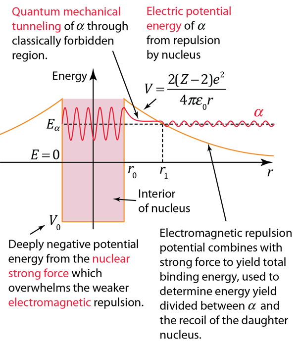
Fig. 6.9 The nuclear strong force and the electromagnetic force influence radioactivity in the form of alpha decay. Image credit: Hyperphysics#
The alpha particle is trapped inside the nucleus and classically, it does not have enough energy to penetrate the Coulomb barrier. Through quantum mechanics, the alpha particle can “tunnel” through the Coulomb potential to escape. The widely varying alpha emission rates can be explained by small changes in the potential barrier (both height and width).
6.8. Homework Problems#
Problem 1
Show directly that the trial wave function \(\Psi (x,t) = e^{i(kx-\omega t)}\) satisfies the time-dependent Schrödinger wave equation.
Problem 2
Normalize the wave function \(Are^{-r/a}\) from \(r=0\) to \(\infty\), where \(\alpha\) and \(A\) are constants. See Wolfram alpha for help with difficult integrals and/or mathematical functions.
Problem 3
A wave function has the value \(A \sin{x}\) for \(0\leq x \leq \pi\), but zero elsewhere. Normalize the wave function and find the probability for the particle’s position: (a) \(0\leq x \leq \pi/4\) and (b) \(0\leq x \leq \pi/2\).
Problem 4
Determine the average value of \(\psi^2_n(x)\) inside an infinite square-well potential for \(n = 1,\ 5,\ 10,\ \text{and}\ 100\). Compare these averages with the classical probability of detecting the particle inside the box.
Problem 5
Compare the results of the infinite and finite square-well potentials.
(a) Are the wavelengths longer or shorter for the finite square well compare with the infinite well?
(b) Use physical arguments to decide whether the energies (for a given quantum number \(n\)) are larger or smaller for the finite square well compared to the infinite square well.
Problem 6
Write the possible (unnormalized) wave functions for each of the first four excited energy levels for the cubical box.
Problem 7
Check to see whether the simple linear combination of sine and cosine functions (\(\psi = A\sin(kx) + B\cos(kx)\)) satisfies the time-independent Schrödinger equation for a free particle (\(V=0\)).