5. Quantum Mechanics: Part I#
5.1. X-Ray Scattering#
Röntgen’s discovery of x-rays excited efforts to determine the nature and origin of the new penetrating radiation. in the early 1900s, Charles Barkla discovered that each elements x-rays of characteristic wavelengths and that x-rays exhibit properties of polarization.
It became clear that x-rays had wave properties and were a form of EM radiation. X-ray wavelengths are much shorter than those of visible light, which made it difficult to refract or diffract them like earlier experiments with visible light. Wien and Sommerfeld had estimated the wavelength of an x-ray to be \(0.01-0.1\ {\rm nm}\). Knowing the distance between atoms in a crystal (\(\sim 0.1\ {\rm nm}\)), Max von Laue made the suggestion that x-rays should scatter from the atoms of crystals. He proposed that if x-rays were a form of EM radiation, then interference effects should be observed. Furthermore, he identified that crystals might act as three-dimensional gratings that could scatter thew waves and produce the observable interference effects.
Note
From the study of optics, we know that wave properties are most easily demonstrated when the sizes of apertures or obstructions are on the same order as the wavelength of light. We use gratings in optics to separate light by diffraction into different wavelengths.

Fig. 5.1 Image credit: PhysicsOpenLab#

Fig. 5.2 The Laue diagram of a NaCl (100) single crystal with a face-center cubic crystal lattice (fcc). Image credit: PhysicsOpenLab#
von Laue designed an experiment to perform a test his hypothesis. He convinced his assistants (Walter Friedrich and Paul Knipping) to perform the measurement. When they rotated the crystals, the positions and intensities of the diffraction were shown to change. Though the purposed of von Laue’s experiment was to prove the wave nature of x-rays, he demonstrated the lattice structure of crystals too. The lattice structure of crystals led to the origin of solid-state physics and the development of modern electronics.
William Henry Bragg and his son, William Lawrence Bragg, fully exploited the wave nature of x-rays and simplified von Laue’s analysis. Bragg (the son) pointed out that each of the images surrounding the bright central spot of von Laue’s photographs could be the reflection of the incident x-ray beam from a unique set of atoms within the crystal. Each dot in the pattern corresponds to different ste of planes in the crystal.
Is x-ray scattering from atoms within crystals consistent with what we know from classical physics? From classical EM theory, we know that the oscillating electric field polarizes an atom. The result is an asymmetric chared distribution, or electric dipole. An electric dipole that oscillates at same frequency as the incident wave will in turn re-radiate EM radiation at the same frequency in the form of spherical waves. The spherical waves travel through the crystal, constructively or destructively interfering as the waves pass through different directions in the crystal.
Fig. 5.3 The crystal structure of \(\rm NaCl\) (rock salt) showing two of the possible sets of Bragg planes. Image credit: OpenStax: University Physics Vol 3#
Consider x-rays scattered from a rock salt crystal (\(\rm NaCl\)). Through Bragg’s simplification, we can determine the conditions necessary for constructive interference. Lattice planes (or Bragg planes) exist within the crystal structure of \(\rm NaCl\), where an incident plane wave (of wavelength \(\lambda\)) can scatter from two adjacent planes. There are two conditions for constructive interference of the x-rays:
The angle of incidence must equal the angle of reflection of the outgoing wave (i.e., from optics).
The difference in path lengths \((2d\sin \theta)\) must be an integral number of wavelengths.
Condition 2 is known as Bragg’s law and can be written mathematically by
which depends on the distance \(d\) between lattice planes (or interatomic spacing). The integer \(n\) is called the order of reflection, following from the terminology of ruled diffraction gratings in optics.
Fig. 5.4 X-ray diffraction with a crystal. Two incident waves reflect off two planes of a crystal. The difference in path lengths is indicated by the dashed line. Figure credit: OpenStax: University Physics Vol 3#
Bragg’s law is useful for determining either the wavelength \(\lambda\) of the x-rays or the interplanar spacing \(d\) (if \(\lambda\) is known). The Braggs (father and son) shared the 1915 Nobel Prize. A Bragg spectrometer measures how x-rays are scattered in a crystal, where the intensity of the diffracted beam is determined as a function of the scattering angle by rotating the crystal and detector.

Fig. 5.5 Schematic of a Bragg spectrometer. X-rays are produced by electron bombardment of a metal target within the x-ray tube. The x-rays are collimated by lead, scatter from a crystal, and are detected as a function of the angle \(2\theta\). Image credit: Hyperphysics#
von Laue diffraction is primarily used to determine the orientation of single crystals by mounting large crystals in a precisely known orientation. White light (i.e., light containing many colors) is projected parallel to a high symmetry direction of the crystal, where arrays of interference maxima spots are produced to indicate a particular plane in the crystal. Bragg and von Laue x-ray diffraction techniques tell su almost everything we know about the structures of solids liquids and even DNA.
Small crystals can be ground into a powdered form, where the small crystals will then have random orientations. When a beam of x-rays passes through the powder, the interference maxima appear as a series of rings. This process is called powder x-ray diffraction (XRD) and is widely used (in crystallography) to determine the structure of unknown solids.
Exercise 5.1
X-rays scattered from rock salt \((\rm NaCl)\) are observed to have an intense maximum at an angle of \(20^\circ\) from the incident direction. Assuming \(n=1\) (from the intensity), what must be the wavelength of the incident direction?
To find \(\lambda\), we can use Bragg’s law (Eqn. (5.1)). We need to know the lattice spacing \(d\) and the angle \(\theta\). The angle for the maximum intensity corresponds to the angle needed for constructive interference, which is always \(2\theta\). Therefore, we have \(\theta = 10^\circ\). The density \(\rho\) of \(\rm NaCl\) is \(2.16\ {\rm g/cm^3}\) and its molar mass \(M\) is \(58.5\ {\rm g/mol}\). These values are needed to find the lattice spacing \(d\), where the relation to Avogadro’s number \(N_A\) to number density was shown in Section 4.1. The number density of \(\rm NaCl\) is
Since \(\rm NaCl\) has a cubic array, we take \(d\) as the lattice spacing, where
This technique for calculating lattice spacing works only for a few cases because of the variety of crystal structures (many of which are noncubic). Now, we can use Bragg’s law to find \(\lambda\) (with \(n=1\)) as
which is a typical x-ray wavelength. \(\rm NaCl\) is a useful crystal for determining x-ray wavelengths and for calibrating an experimental apparatus.
5.2. De Broglie Waves#
By 1920 it was clear that x-rays exhibited wave properties, where x-ray crystallography could be used to study the crystalline structure of atoms and molecules. A detailed understanding of the atom was not yet proposed, where a more general theory was necessary to replace the Bohr model of the atom. A first step was made by Prince Louis deBroglie, who was well versed in the work of Planck, Einstein, and Bohr. De Broglie was struck by how photons (EM radiation) had both wave (e.g., crystallography) and particle (e.g., photoelectric effect) properties. If electromagnetic radiation must have both wave and particle properties, they material particles should have both wave and particle properties as well. According to de Broglie, the symmetry of nature encourages such an idea, and no laws of physics prohibit it.
De Broglie presented his new hypothesis within his doctoral thesis to the University of Paris in 1924, where it aroused both interest and skepticism. De Broglie combined the special theory of relativity with quantum theory to establish the wave properties of particles. He predicted a relationship between the wavelength \(\lambda\) and momentum \(p\) for a particle as
De Broglie was guided by the concepts of phase and group velocities of waves. Recall that photons have energy through momentum \(E= pc\) and with a frequency \(E=hf\), so that
De Broglie extended his relation for photons to all particles. Particle (or matter) waves have a momentum and act as a particle through a wavelength called the de Broglie wavelength.
How do we show whether an object can exhibit wavelike properties? The best way is to pass them through a slit that has a width of a similar dimension as the object’s wavelength. It is virtually impossible for a tennis ball to demonstrated interference or diffraction because its wavelength is \(\sim 10^{-34}\ {\rm m}\). But the de Broglie wavelength of a \(50\ {\rm eV}\) electron is about \(0.2\ {\rm nm}\), which is large enough that we can demonstrate its wave properties. Because of their small mass, electrons can have a small momentum and in turn a large wavelength \((\lambda = h/p)\).
Exercise 5.2
Calculate the de Broglie wavelength of a (a) tennis ball (\(m = 57\ {\rm g}\)) traveling \(25\ {\rm m/s}\) and (b) \(50\ {\rm eV}\) electron.
(a) For the tennis ball, we need to calculate its momentum \(p=mv\) and substitute into
(b) For the electron, we need to calculate its momentum in terms of the kinetic energy \(K\) (i.e., \(p=\sqrt{2mK}\)). The kinetic energy can be converted from \(\rm eV\) to \(J\) or the rest mass can be converted from \(\rm kg\) to \(\rm eV\). Both methods give the same result. The de Broglie wavelength is calculated as
from scipy.constants import h,c,e,m_e,eV,physical_constants
import numpy as np

def deBroglie_wave(p,unit):
    #calculate the de Broglie wavelength
    if unit == 'kg':
        return h/p
    else:
        return hc/p #using units of eV for mass; need hc in eV*m

m_tb = 0.057 #mass of tennis ball in kg
v_tb = 25 #speed of tennis ball in m/s

hc = h*c/eV
me_eV = physical_constants['electron mass energy equivalent'][0]/eV
K_eV = 50 #kinetic energy of electron in eV
K_J = 50*eV #kinetic energy of electron in J

#part a
l_tb = deBroglie_wave(m_tb*v_tb,'kg')
print("The de Broglie wavelength of the tennis ball is %1.2e m.\n" % (l_tb))

#part b
l_e = deBroglie_wave(np.sqrt(2*m_e*K_J),'kg')
print("The de Broglie wavelength of the electron (using kg and J) is %1.2e m.\n" % l_e)

l_e = deBroglie_wave(np.sqrt(2*me_eV*K_eV),'eV')
print("The de Broglie wavelength of the electron (eV) is %1.2e m.\n" % l_e)
The de Broglie wavelength of the tennis ball is 4.65e-34 m.

The de Broglie wavelength of the electron (using kg and J) is 1.73e-10 m.

The de Broglie wavelength of the electron (eV) is 1.73e-10 m.
5.2.1. Bohr’s Quantization Condition#
In the hydrogen atom model, Bohr assumed that the electron’s angular momentum is quantified through an integral multiple of \(\hbar\). De Broglie comes to the same assumption by representing the electron as a standing wave in an orbit around the proton. The condition for a standing wave is that the entire length of the wave mus fit within the orbit’s circumference (i.e., standing waves in a closed pipe). For a standing wave, we must have
given the radius of the orbit \(r\). Using the de Broglie relation for the wavelength, we produce
The angular momentum of the electron in this orbit is \(L=mvr=rp\), and then we have
This is Bohr’s quantization assumption generated by applying de Broglie’s wavelength for an electron in a standing wave. This result appears to justify Bohr’s assumption.
5.3. Electron Scattering#
In 1925, Clinton Davisson and Lester Germer were investigating the properties of metallic surfaces by scattering electrons from various materials when a liquid air bottle exploded near their apparatus. The nickel target was at a high temperature at the time of the accident, and the breakage of their vacuum system caused significant oxidation of the nickel. After repairing their apparatus, Davisson and Germer found a striking change in the way electrons were scattering from the nickel surface. Previously, they measured a smooth variation of intensity with scattering angle, but the new data showed large numbers of scattered electrons for certain energies at a given scattering angle.
Davisson and Germer found that the high temperature had modified the polycrystalline structure of the nickel. The many small crystals of the original target were changed into a few large crystals as a result of the heat treatment. Davisson deduced that it was the new arrangement of the nickel atoms that had caused the new intensity distributions. The electrons were diffracted much like x-rays, and Davisson found that Bragg’s law applied to their data. Davisson and Germer varied both the scattering angles (for a given wavelength) and the wavelength (for a given angle). In Bragg’s law the angle between the incident and scattered beams is \(2\theta\), where Davisson and Germer found the angle between the incident and scattered beams as \(\phi =2\alpha\). The angle \(\theta\) from Bragg’s law is different from \(\alpha\) by \(90^\circ\) (i.e., \(\theta -\alpha = \pi/2\)). We can then show from trigonometric identities that
This allows us to rewrite the Bragg condition as
Bragg’s law is written in terms of the lattice plane spacing \(d\), where we want to know the interatomic distance \(D\) and have the relation \(d= D\sin \alpha\). Applying to Bragg’s law, we find
For nickel the interatomic distance is \(D=0.215\ {\rm nm}\). Davisson and Germer found an electron scattering peak at \(\phi = 50^\circ\), then the electron wavelength should be \(\lambda = (0.215\ {\rm nm})\sin 50^\circ = 0.165\ {\rm nm}\).
Shortly after Davisson and Germer reported their experiment, many others showed the effects of electron diffraction in transmission experiments. The targets were varied including celluloid, gold, aluminum, and platinum. Davisson and George Thomson received the Nobel Prize in 1937, which clearly showed that particles exhibit wave properties.
Exercise 5.3
Assuming that the de Broglie wavelength of the electron is \(0.165\ {\rm nm}\) from the Davisson and Germer experiment. What is the kinetic energy of the electron in eV?
Using the equation for the de Broglie wavelength, we can find the momentum \(p\) of the electron by
The kinetic energy can be written in terms of the momentum by
Davisson and Germer used \(54\ {\rm eV}\) electrons, which shows that massive particles can behave like waves.
from scipy.constants import h,m_e,eV

def kinetic_energy(l,m):
    #calculate the kinetic energy (in J) of a particle of mass m using its de Broglie wavelength
    #l = wavelength in m
    p = h/l
    return p**2/(2*m)

l_e = 1.65e-10 #electron de Broglie wavelength from Davisson-Germeer
KE_e = kinetic_energy(l_e,m_e)
print("The kinetic energy of the electron from the Davisson-Germer experiment is %1.2e J or %2.1f eV." % (KE_e,KE_e/eV))
The kinetic energy of the electron from the Davisson-Germer experiment is 8.85e-18 J or 55.2 eV.
Exercise 5.4
An ideal gas (or particle) in thermal equilibrium with its surroundings has a kinetic energy of \(3kT/2\) (see Sect. 1.2.2). Calculate the de Broglie wavelength for a: (a) neutron at room temperature (\(300\ {\rm K}\)) and (b) “cold” neutron at \(77\ {\rm K}\) (liquid nitrogen).
From Section 1.2.2, the internal energy \(U\) is equivalent to the kinetic energy \(\text{K.E.}\) of an ideal gas. Written in terms of the momentum \(p\) gives,
which can be solved to get \(p = \sqrt{3m_NkT}\) using the mass \(m_N\) of a neutron. With the momentum, we can write the de Broglie wavelength as
(a) For a neutron at room temperature, its de Broglie wavelength is calculated as
(b) For a neutron at \(77\ {\rm K}\), its de Broglie wavelength is
These wavelengths are suitable for diffraction by crystals. “Supercold” neutrons are useful because extraneous electric and magnetic field do not affect neutrons nearly as much as electrons.
from scipy.constants import h, m_n, k
import numpy as np

def deBroglie_wave_gas(T):
    #calculate de Broglie wavelength in m for a particle in an ideal gas
    #T = temperature in Kelvin
    p = np.sqrt(3*m_n*k*T)
    return h/p
T_room = 300 #room temperature in K
l_room = deBroglie_wave_gas(T_room)
print("The de Broglie wavelength of a neutron at room temperature is %1.3e m or %1.3f nm.\n" % (l_room,l_room/1e-9))

T_cold = 77 #cold temperature in K
l_cold = deBroglie_wave_gas(T_cold)
print("The de Broglie wavelength of a neutron at 77 K is %1.3e m or %1.3f nm.\n" % (l_cold,l_cold/1e-9))
The de Broglie wavelength of a neutron at room temperature is 1.452e-10 m or 0.145 nm.

The de Broglie wavelength of a neutron at 77 K is 2.867e-10 m or 0.287 nm.
5.4. Wave Motion#
It must be possible to formulate a wave description of particle motion because both massless and massive particles exhibit wave behavior. The quantum of theory of physics is based heavily on waves, where we develop a framework for waves before applying it to particles.
The simplest form of a wave has a sinusoidal form, and at an initial time \(t=0\), its spatial variation (as a function of \(x\)) looks like
in terms of the wave number \(k=2\pi/\lambda\) and maximum displacement \(A\) (or amplitude). The wavelength \(\lambda\) is defined as the distance between two points on the wave with the same value of \(\Psi\). The time required for a wave to travel one wavelength \(\lambda\) is called the period \(T\).
Note
The term “wave number” has two common usages. Spectroscopists use “wave number” to mean the reciprocal of the wavelength (\(1/\lambda\)), or the number of waves that fit into a meter of length. The other convention is to use a length \(2\pi\) instead to get \(k=2\pi/\lambda\).
A wave with \(t=\text{const.}\) is also called a stationary wave because it is constant in time. The function of \(\Psi(x,t)\) represents the instantaneous amplitude (i.e., displacement) of the wave at a time \(t\). In the case of
a traveling wave moving down a string, \(\Psi\) is the displacement of the string from equilibrium.
the electric field \(\vec{E}\) or magnetic field \(\vec{B}\), \(\Psi\) is the magnitude of the respective field.
As time increases, the position of the wave will change so the general expression for the wave is
Show code cell source
import numpy as np
import matplotlib.pyplot as plt
from matplotlib import rcParams

rcParams.update({'font.size': 18})
rcParams.update({'mathtext.fontset': 'cm'})

def sine_wave(x,l,v,t):
    #calculate the displacement Psi of a sine wave at a particular time t
    #x = position (in m)
    #l = wavelength (in m)
    #v = phase velocity (in m/s)
    #t = time (in s)
    return np.sin((2.*np.pi/l)*(x - v*t))

fs = 'medium'
lw = 2
col = (218/256., 26/256., 50/256.)

l_wave = 1 #wavelength in m
v_wave = 5 #mean speed in m/s

x_wave = np.arange(-1,1,0.001)

fig = plt.figure(figsize=(6,3),dpi=150)
ax = fig.add_subplot(111)

psi_o = sine_wave(x_wave,l_wave,v_wave,0) #displacement Psi at t=0 s
T = 0.25*v_wave/l_wave
psi_t = sine_wave(x_wave,l_wave,v_wave,T) #displacement Psi at t=1.25 s
ax.plot(x_wave,psi_o,'k-',lw=lw,label='$\Psi(x,0)$')
ax.plot(x_wave,psi_t,'--',color=col,lw=lw,label='$\Psi(x,1.25)$')
ax.legend(loc='upper center',ncol=2,fontsize=fs)

ax.set_ylabel('$\Psi(x,t)$',fontsize=fs)
ax.set_xlabel('$x$')

ax.set_ylim(-1.1,2.)
ax.set_xticks([])
ax.set_yticks([]);
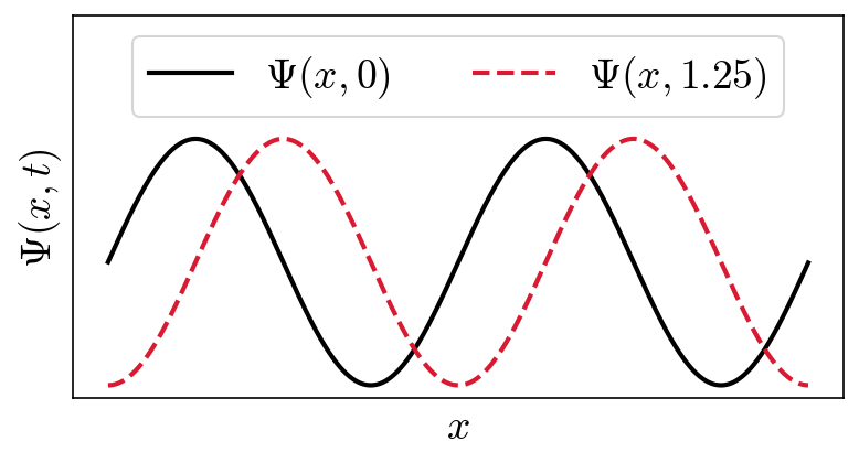
The above figure shows two waves with the same frequency and amplitude, but they are displaced in time by \(1.25\ {\rm s}\), or shifted by a quarter-phase. Click the button on the right to show the python code underlying the figure.
The phase velocity \(v\) is related to the wavelength \(\lambda\) and period \(T\) through the relation \(\lambda = vT\). The frequency (\(f = 1/T\)) of a harmonic wave is the number of times a wave crest passes a given point (i.e., a complete cycle). A traveling wave satisfies the wave equation:
Using \(\lambda = vT\) , we can Eqn. (5.7) as
where the angular velocity is \(\omega= 2\pi/T\) and
This is the mathematical description of a sine curve traveling in the positive \(x\) direction that has a zero-displacement (\(\Psi = 0\)) at \(x=0\) and \(t=0\). A similar wave traveling in the negative \(x\) direction has the form
The phase velocity \(v_{\rm ph}\) is the velocity for a point on the wave that has a given phase (e.g., the crest), which is
A wave can be shifted by a phase constant \(\phi\), which produces
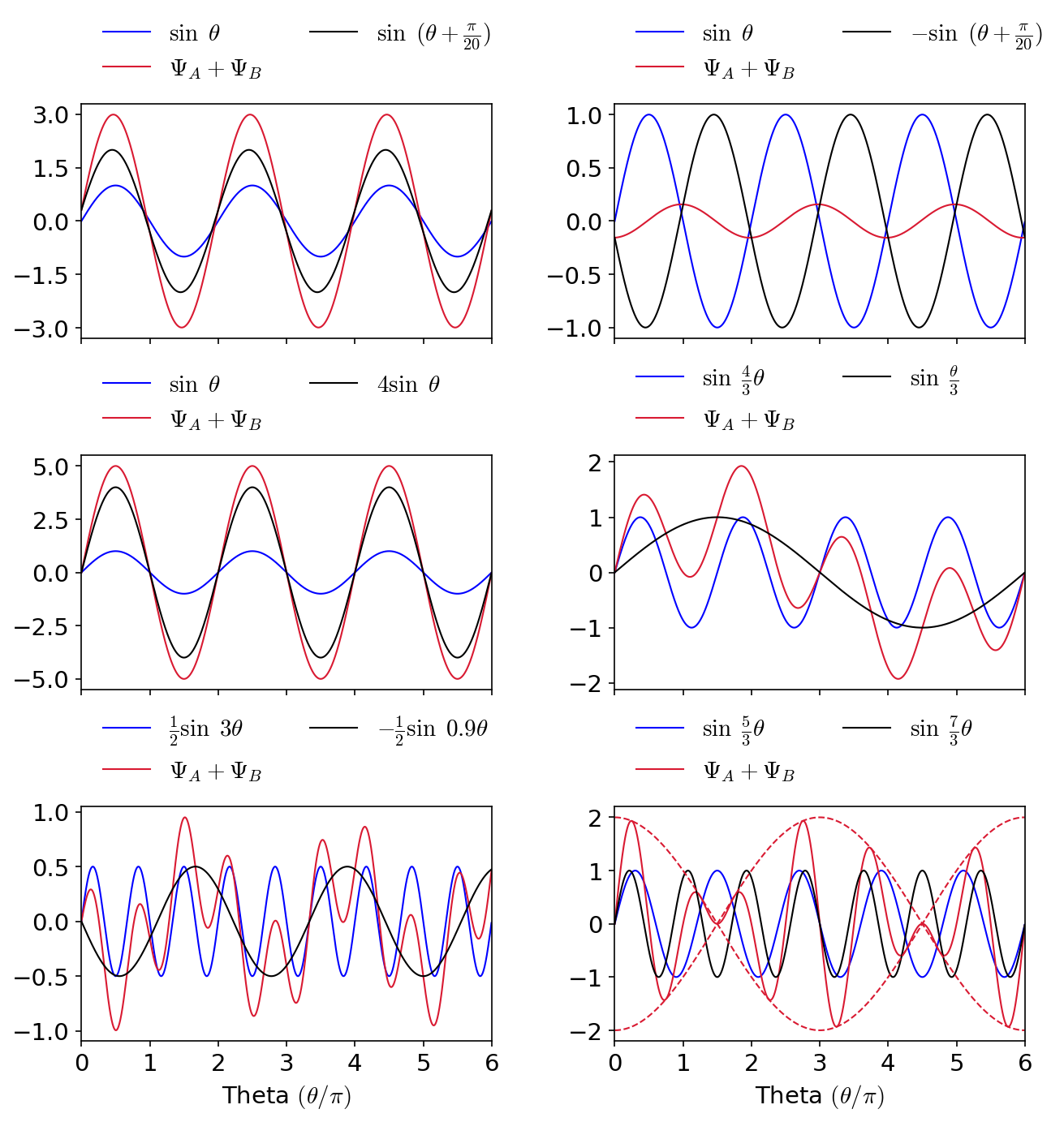
When two or more waves traverse the same region, then they act independently of each other. We add the displacements of all the waves present through the principle of superposition. For sound, beating occurs when two waves have nearly equal frequencies. The net displacement depends on the harmonic amplitude, phase, and frequency of each individual wave. Combining waves is accomplished by adding their instantaneous displacements.
The figure below illustrates of two waves \(\Psi_A\) (blue), \(\Psi_B\) (black), and their superposition \(\Psi_A + \Psi_B\) (red). Depending on the relative phase and amplitude of \(\Psi_A\) or \(\Psi_B\), the resulting wave can be larger or smaller in overall amplitude. The bottom-right panel shows the phenomenon of beats (dashed red), which is the envelope of maximum displacement of the combined waves. Click the button on the right to show the python code underlying the figure.
Show code cell source
import numpy as np
import matplotlib.pyplot as plt
from matplotlib.ticker import MaxNLocator
from matplotlib import rcParams

rcParams.update({'font.size': 14})
rcParams.update({'mathtext.fontset': 'cm'})

def sine_wave(th,ph,A):
    #calculate the displacement Psi of a sine wave at a particular time t
    #th = angle
    #ph = phase offset
    #A = amplitude
    return A*np.sin(th+ph)

fs = 'medium'
lw = 1
col = (218/256., 26/256., 50/256.)
theta = np.arange(0,6*np.pi,0.01)

fig = plt.figure(figsize=(10,10),dpi=150)
ax11 = fig.add_subplot(321)
ax12 = fig.add_subplot(322)
ax21 = fig.add_subplot(323)
ax22 = fig.add_subplot(324)
ax31 = fig.add_subplot(325)
ax32 = fig.add_subplot(326)
ax_list = [ax11,ax12,ax21,ax22,ax31,ax32]

theta_A = [1,1,1,4./3,3.,5./3]
theta_B = [1,1,1,1./3.,0.9,7./3]
Amp_A = [1,1,1,1,0.5,1]
Amp_B = [2,-1,4,1,-0.5,1]
label_A = ['$\sin\  \\theta$','$\sin\ \\theta$','$\sin\ \\theta$','$\sin\ \\frac{4}{3}\\theta$','$\\frac{1}{2}\sin\ 3\\theta$','$\sin\ \\frac{5}{3}\\theta$']
label_B = ['$\sin\ (\\theta+\\frac{\pi}{20})$','$-\sin\ (\\theta+\\frac{\pi}{20})$','$4\sin\ \\theta$','$\sin\ \\frac{\\theta}{3}$','$-\\frac{1}{2}\sin\ 0.9\\theta$','$\sin\ \\frac{7}{3}\\theta$']

for i in range(0,6):
    ax = ax_list[i]
    ph_off = 0
    if i <2:
        ph_off = np.pi/20.

    Psi_A = sine_wave(theta_A[i]*theta,0,Amp_A[i])
    Psi_B = sine_wave(theta_B[i]*theta,ph_off,Amp_B[i])
    Psi_AB = Psi_A + Psi_B

    ax.plot(theta/np.pi,Psi_A,'b-',lw=lw,label=label_A[i])
    ax.plot(theta/np.pi,Psi_AB,'-',color=col,lw=lw,label='$\Psi_A + \Psi_B$')
    ax.plot(theta/np.pi,Psi_B,'k-',lw=lw,label=label_B[i])
    if i == 5:
        k_diff = (theta_A[i]-theta_B[i])/2
        Psi_beat = sine_wave(k_diff*theta,np.pi/2.,2)
        ax.plot(theta/np.pi,Psi_beat,'--',color=col,lw=lw)
        ax.plot(theta/np.pi,-Psi_beat,'--',color=col,lw=lw)

    ax.set_xlim(0,6)
    ax.set_xticks(range(0,7))
    if i<4:
        ax.set_xticklabels([])
    else:
        ax.set_xlabel("Theta $(\\theta/\pi)$",fontsize=fs)
    ax.yaxis.set_major_locator(MaxNLocator(5))
    ax.legend(bbox_to_anchor=(0., 1.01, 1., .102),ncol=2,fontsize=14,frameon=False)

fig.subplots_adjust(hspace=0.5,wspace=0.3);
In quantum mechanics, waves are used to represent a moving particle. For different amplitudes and frequencies, it is possible to obtain a wave packet. An important property of a wave packet is that its net amplitude is nonzero over a small region \(\Delta x\). This localizes the position of a particle to a particular region.
Fig. 5.6 If discrete traveling wave solutions to the wave equation are combined, they can be used to create a wave packet which begins to localize the wave. Figure credit: Hyperphysics#
Consider two waves of equal harmonic amplitude \(A\), but different wave numbers (\(k_1\) and \(k_2\)) and angular frequencies (\(\omega_1\) and \(\omega_2\)). The superposition of the two waves is the sum
Each wave \(\Psi_1\) and \(\Psi_2\) can be transformed to \(\cos \alpha\) and \(\cos\ \beta\), where \(\alpha = k_1x-\omega_1t\) and \(\beta = k_2x -\omega_2 t\) with appropriate subscripts. Using the trigonometric identity for cosine:
we can obtain
The average wave number \(k_{\rm av}\) and average angular frequency \(\omega_{\rm av}\) modulates one wave, while the difference in wave number \(\Delta k\) and angular frequency \(\Delta \omega\) affects the other. The full superposition is the product of the combination of wave components. The individual waves \(\Psi_1\) and \(\Psi_2\) move with their own respective phase velocity \(\omega_1/k_1\) and \(\omega_2/k_2\), while the combined wave has a phase velocity \(\omega_{\rm av}/k_{\rm av}\). Combining more than two waves produces a pulse, or wave packet, which moves at the group velocity (\(u_{\rm gr} = \Delta\omega/\Delta k\)).
The combination of only two waves is not localized in space. However, a “localized region” \(\Delta x = x_2-x_1\) can exist where the envelope is zero (or maximum). The term \(\Delta kx/2\) must be different by a phase of \(\pi\) for the values \(x_1\) and \(x_2\), because \(x_2 - x_1\) represents only a half-wavelength of the envelope that confines the wave, or
A similar reasoning can be applied to determine a time \(\Delta t\) over which the wave is localized and obtain \(\Delta \omega \Delta t = 2\pi\).
The relation (in Eqn. (5.16)) implies that to determine a precise position \(\Delta x\) of the wave packet (\(\Delta x \rightarrow \text{small}\)), we must have a large range of wave numbers (\(\Delta k \rightarrow \text{large}\)). A similar reasoning can be applied for the relation between angular frequency and time.
Equation (5.14) can be extended to consider the sum over many waves with possibly different wave numbers, angular frequencies, and amplitudes through a Fourier series, or
Gaussian wave packets are often used to represent the position of particles because the associated integrals are relatively easy to evaluate. A Gaussian wave (at \(t = 0\)) can be expressed as
where the range of wave numbers \(\Delta k\) are used to form the wave packet. The \(\cos(k_o x)\) term describes an oscillating wave within the (Gaussian) exponential envelope \(e^{-\Delta k^2 x^2}\). The figure below shows an intensity distribution \(\mathcal{I}(k)\) described by a Gaussian (on the left) and a corresponding wave packet \(\psi(x)\) (on the right). Click the button on the right to show the python code underlying the figure.
Show code cell source
import numpy as np
import matplotlib.pyplot as plt

def gaussian(x,s,m):
    #Calculate a gaussian
    #A = amplitude (height) of the curve
    #s = standard deviation
    #m = position of the central peak
    return np.exp(-0.5*(x-m)**2/s**2)/np.sqrt(2.*np.pi*s**2)

A_k = 1
delta_k = 0.25
k_o = 2.*np.pi/2.
col = (218/256., 26/256., 50/256.)

fs = 'medium'
lw = 2

k = np.arange(0.8*np.pi,1.2*np.pi,0.001)
x = np.arange(-2*np.pi,2.*np.pi,0.001)
I_k = gaussian(k,delta_k,k_o)
psi_gauss = np.exp(-delta_k**2*x**2)
psi_wave = np.cos(k_o*x)
psi_x = A_k*psi_gauss*psi_wave
delta_x = np.std(psi_x)

fig = plt.figure(figsize=(8,4),dpi=150)
ax1 = fig.add_subplot(121)
ax2 = fig.add_subplot(122)

ax1.plot(k,I_k,'-',color=col,lw=lw)
ax1.axvline(np.pi,color='k',linestyle='--',lw=lw)

ax2.plot(x,psi_x,'k--',lw=lw,label='$\cos\ k_o x$')
ax2.plot(x,psi_gauss,'-',color=col,lw=lw,label='$e^{-\Delta k^2 x^2}$')
ax2.plot(x,-psi_gauss,'-',color=col,lw=lw)
ax2.legend(bbox_to_anchor=(0., 1.01, 1., .102),ncol=2,fontsize=fs,frameon=False)


ax1.set_yticks([])
ax1.set_xticks([3.14])
ax1.set_ylabel("$\mathcal{I}(k)$",fontsize=fs)
ax1.set_xticklabels(['$k_o$'])

ax2.set_yticks([])
ax2.set_xticks([0])
ax2.set_ylabel("$\psi(x)$")
ax2.set_xticklabels(['$x_o$'])

fig.subplots_adjust(wspace=0.2);
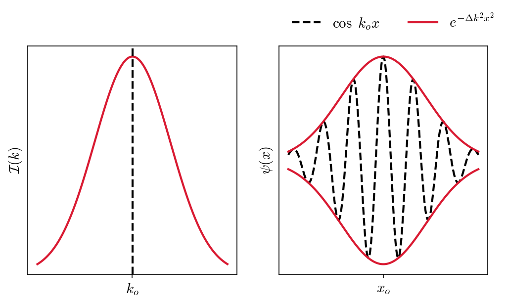
For the intensity distribution, there is a high probability of a particular measurement of \(k\) begin within one standard deviation \(\sigma\) from the mean value \(k_o\). For the wave packet \(\psi(x)\) there is a good probability of finding the particle near \(x_o\) and within one standard deviation.
We must be convinced that the superposition of waves can actually describe particles. The superposition of waves produces a group velocity \(u_{\rm gr} = \Delta\omega/\Delta k\) that represents the motion of the envelope. The group velocity can be generalized so that \(\Delta \rightarrow d\) to give
For a de Broglie wave, we know \(E= hf\) and \(p = h/\lambda\). We can rewrite these equations in terms of \(\hbar\) as,
If we multiply Eqn. (5.19) by \(1 = \hbar/\hbar\), we have
Recall the relativistic energy relation \(E^2 = p^2c^2 + m^2c^4\) and evaluate its derivative to get
or
Equation (5.21) represents a particle with a momentum \(p\) and total energy \(E\). It is plausible to assume that the group velocity of the wave packet can be associated with the particle velocity. The phase velocity is represented by
so that \(\omega = kv_{\rm ph}\). Then, the group velocity is related to the phase velocity by
The group velocity may be greater or less than the phase velocity. If the phase velocity is the same for all frequencies, then the medium is nondispersive and \(u_{\rm gr} = v_{\rm ph}\) (e.g., an electromagnetic wave in vacuum; Fig. 5.7).
Fig. 5.7 Propagation of a wave packet in a non-dispersive medium, where there is no difference between phase velocity and group velocity. Image credit: Wikipedia#
Fig. 5.8 Propagation of a wave packet in a dispersive medium, where there is a difference between phase velocity and group velocity. Image credit: Wikipedia#
Water waves are a good example of waves in a dispersive medium (Fig. 5.8). Dispersion plays a role in the shape of wave packets, where they can spread out as time progresses.
Exercise 5.5
Newton showed that deep-water waves have a phase velocity of \(\sqrt{g\lambda/(2\pi)}\). Find the group velocity of such waves and discuss the motion.
Starting with Eqn. (5.23), we see that it is dependent on the wave number \(k\) and need to convert the phase velocity from \(\lambda\) to \(k\). Using \(\lambda = 2\pi/k\), we have
Now, we can take the necessary derivative to get
The group velocity is one-half the phase velocity. Such an effect can be observed by throwing a rock in a still pond. As the circular waves move out, the individual waves seem to run right through the wave crests and then disappear.
5.5. Waves or Particles#
Electromagnetic radiation behaves sometimes as waves (e.g., interference and diffraction) and other times as particles (e.g., photoelectric and Compton effects). In addition, there is evidence that massive particles also behave as waves (e.g., electron diffraction). Wave-particle duality leads to a few questions:
If a particle is a wave, what is waving?
Can we represent matter as waves and particles simultaneously?
Can we represent EM radiation as waves and particles simultaneously?
5.5.1. Double-Slit Experiment with Light#
Young’s double-slit diffraction experiment show the interference character of light. This experiment is easily performed with a monochromatic light source (i.e., a laser). With both slits open, an interference patter is observed with bands of maxima and minima. With one slit covered the interference pattern is changed and broad peak is observed (i.e., the envelope in Fig. 5.9). We conclude that the double-slit interference pattern is due to light passing through both slits, which is a wave phenomenon.
Fig. 5.9 The interference pattern for a double slit has an intensity that falls off with angle. The image shows multiple bright and dark lines, or fringes, formed by light passing through a double slit. Image credit: OpenStax: University Physics Vol 3#
If the light intensity is reduced, we find that the light arriving on the screen produces flashes at various points and is indicative of particle behavior. Eventually (with enough counts) the interference patter characteristic of wave behavior emerges. There is no contradiction in this experiment. See the video below for an explanation from the Christmas lectures by the Royal Institution.
5.5.2. Electron Double-Slit Experiment#
A similar double-slit experiment can be performed using electrons rather than light. If matter behaves as waves, then the same experimental results should be obtain using electrons. This experiment isn’t as easy to perform due to the difficulty in constructing slits narrow enough to exhibit wave phenomena (recall that electron diffraction was first performed at short wavelengths \(\lambda \sim 0.2\ {\rm nm}\)).
In 1961, Claus Jönsson succeeded in showing double-slit interference effects for electrons by constructing very narrow slits and using relatively large distance between the slits and the observation screen. Copper slits were made by electrolytically depositing copper on a polymer strip printed on silvered glass plates. This experiment demonstrated that both wave and particle behaviors can be seen for both light and electrons. See the paper.
Exercise 5.6
In the experiment by Jönsson, \(50\ {\rm keV}\) electrons were directed onto slits that are \(500\ {\rm nm}\) wide and separated by \(2\ \mu{\rm m}\). The observation screen is located \(0.35\ {\rm m}\) beyond the slits. What was the distance between the first two maxima?
The equation that relates the orders of maxima and the angle \(\theta\) (from incidence) is given by
The first maximum occurs for \(n=0\) and \(\theta = 0\), where the next maximum occurs for \(n=1\) and the angle can be written as
We need to find the wavelength \(\lambda\) of the electrons and then we can determine the distance \(d\) between the two maxima (\(y_1 = D \tan \theta_1\)). From Section 5.2, we can calculate the de Broglie wavelength relativistically by first using Eqn. (2.56) to determine \(pc\) by
Then we can apply the equation for the de Broglie wavelength as
Now we can determine the \(\sin \theta_1\) as
For \(\sin \theta \ll 1\), \(\tan \theta \approx \sin \theta\). The distance \(y_1\) can be calculated as
Such a diffraction pattern is too small to be seen with the naked eye, where Jönsson magnified the pattern by a series of electronic lenses. He then observed a fluorescent screen with a \(10\times\) optical microscope to see the diffraction pattern.
import numpy as np
from scipy.constants import physical_constants,eV,h,c

d_slits = 2e-6 #distance between slits in m
n_1 = 1 #order of maximum
D_screen = 0.35 #distance from slits to the screen in m

KE_e = 5e4 #kinetic energy of electrons in eV
m_e = physical_constants['electron mass energy equivalent'][0]/eV #electron rest mass-energy in eV

pc = np.sqrt((KE_e + m_e)**2 - m_e**2)
print("The relativistic energy-momentum of the 50 keV electron is %1.2e eV.\n" % pc)

l_e = (h*c/eV)/pc
print("The relativistic de Broglie wavelength is %1.2e m.\n" % (l_e))

theta_1 = np.arcsin(n_1*l_e/d_slits) #angle to the first maximum
print("The angle to the first maximum is %1.2e.\n" % theta_1)

y_1 = D_screen*np.tan(theta_1)
print("The distance between the first two maxima is %1.2e m or %d nm." % (y_1,y_1/1e-9))
The relativistic energy-momentum of the 50 keV electron is 2.32e+05 eV.

The relativistic de Broglie wavelength is 5.36e-12 m.

The angle to the first maximum is 2.68e-06.

The distance between the first two maxima is 9.37e-07 m or 937 nm.
5.5.3. Another Gedanken (thought) Experiment#
If we were to cover one of the slits, the double-slit interference pattern would be destroyed. But our experiments tell us that the electron is a particle, where it must go through only one of the slits.
Let’s devise a gedanken (thought) experiment, where a light shines on the double slit and we use a powerful microscope. After the electron passes through one of the slits, light bounces off the electron and we can observe the reflected light. Therefore, we know which slit the electron came through.
We need to use light with a wavelength smaller than the slit separation \(d\) to determine which slit the electron went through (i.e., \(\lambda_{\rm ph}<d\)). The momentum of the photon is
The electron must also have a wavelength similar to the slit separation \(d\) to see the interference effects (i.e., \(\lambda_e \sim d\)). The momentum of the electrons will be approximately
The photon momentum is big enough to modify the trajectory of the electron! The attempt to identify which slit the electron is passing through will change the interference pattern. In trying to examine which slit the electron went through, we are examining the particle-like behavior and the wave-like behavior is examined by the interference patter.
Bohr pointed out that the particle-like and wave-like aspects of nature are complementary. Both are needed, where they just can’t be observed simultaneously.
It is not possible to describe physical observables simultaneously in terms of both particles and waves.
—Bohr’s principle of complementarity
5.5.4. Physical Observables#
Physical quantities (e.g., position, velocity, momentum and energy) that can be experimentally measured are physical observables. In experiments, we must use either the particle or wave description. The interference pattern suggests that the light (or electron) had to go through both slits, which naturally calls upon the wave description. We cannot describe phenomena by displaying both particle and wave behavior at the same time.
Note that Bohr’s principle of complementarity is a “principle” and not a “law”. Thus, we use it because it works and are ready to trade it in, if something more suitable comes along. Experiments dictate what actually happens in nature, and we must draw up a set of rules that describe our observations. These rules naturally lead to a probability interpretation of experimental observations.
If we use a series of small detectors along the screen in the electron double-slit experiment, then we can speak of the probability of the electron begin detected. The interference patter can guide our probability determinations, but a detected electron at one of the detectors necessarily forces the probability of it begin seen to zero at the other detectors. Matter and radiation propagation is described by wavelike behavior, but matter and radiation interact as particles.
5.6. Uncertainty Principle#
To localize a wave packet over a small region \(\Delta x\), a large range of wave numbers \(\Delta k\) is necessary. For the case of two waves (or a wave packet), Eqn. (5.16) showed that the product of the \(\Delta k\) and \(\Delta x\) is a constant.
It is impossible to measure the precise values of \(k\) and \(x\) for the same particle, simultaneously. Let’s re-write the wave number \(k\) in terms of the momentum using the relation for the de Broglie wavelength as
In the case of a Gaussian wave packet
or
Equation (5.26) was first presented by Werner Heisenberg, where it applies in all three dimensions and we should include a subscript to indicate the direction. Heisenberg’s uncertainty principle can be written as
which establishes limits on the simultaneous knowledge of \(p_x\) and \(x\). The limits on \(\Delta p_x\) and \(\Delta x\) represent the lowest possible limits on the uncertainties in knowing the values of \(p_x\) and \(x\) (no matter how good an experimental measurement is made). It is possible to have a greater uncertainty in \(p_x\) and \(x\), but their precision is limited by the uncertainty principle.
Note
The uncertainty principle does not apply to products between dimensions (e.g., \(\Delta p_z \Delta x\) or \(\Delta p_y \Delta z\)). The value of \(\Delta p_z \Delta x\) can be zero.
Equation (5.27) is true for all waves (e.g. water, sound, matter, and light) as a consequence of the de Broglie wavelength. If we want to know the position of a particle accurately, we must accept a large uncertainty with the momentum of the particle (either how fast it is moving or how massive it is). The converse is also true. Classical physics assumed that it is possible to specify (simultaneously and precisely) both the particle’s position and momentum, were it is not the case in the quantum realm. Since \(\hbar \ll 1\), the uncertainty principle becomes important only on the atomic level.
Consider a particle for which the location is known within a width of \(\ell\) along the \(x\)-axis. The position of the particle is known within a distance \(\Delta x \leq \ell /2\). Applying the uncertainty principle specifies the limits on momentum \(\Delta p_x\) as
Assume that the mass \(m\) of the particle is precisely known, then \(\Delta p_x = m\Delta v_x\), and
Consider a particle with low energy. What is the minimum kinetic energy the particle can have? Since the energy is low, we can use nonrelativistic equations, where \(K = p^2/(2m)\). Then we can find the minimum value of kinetic energy \(K_{\rm min}\) as
This equation indicates that if we are uncertain as to the exact position of a particle, then the particle can’t have zero kinetic energy.
Exercise 5.7
Calculate the momentum uncertainty of (a) a tennis ball constrained within a fence enclosure of \(35\ {\rm m}\) on a side and (b) an electron with the smallest diameter of a hydrogen atom.
(a) Inserting the uncertainty in the tennis ball’s position, \(\Delta x = (35\ {\rm m})/2\), we have for the momentum uncertainty,
For classical-sized objects, we have no problem specifying the momentum.
(b) The smallest radius of the hydrogen atom is the Bohr radius \(a_o = 5.29 \times 10^{-11}\ {\rm m}\), where the diameter \(d = 2a_o\). The uncertainty in the position of the electron is \(\Delta x = d/2 = a_o\). We have for the momentum uncertainty,
This may seem like a small momentum, but the mass of the electron is also very small. This means that the speed of the electron can be large (Eqn. (5.29)). The minimum speed is \(0.004c\). The minimum kinetic energy is not negligible, where
from scipy.constants import hbar,physical_constants,m_e,c,eV

#part a
delta_x = 35./2 #uncertainty of tennis ball position in m
p_x = hbar/(2*delta_x)
print("The momentum uncertainty is %1.1e kg m/s.\n" % (p_x))

#part b
delta_x = physical_constants['Bohr radius'][0] #radius of the hydrogen atom in m
p_x = hbar/(2*delta_x)
print("The momentum uncertainty is %1.3e kg m/s.\n" % (p_x))

v_x = p_x/m_e
print("The speed of the electron is %1.2e m/s or %1.3f c.\n" % (v_x,v_x/c))

KE_e = p_x**2/(2*m_e)
print("The minimum kinetic energy of the electron is %1.2e J or %1.2f eV." % (KE_e,KE_e/eV))
The momentum uncertainty is 3.0e-36 kg m/s.

The momentum uncertainty is 9.964e-25 kg m/s.

The speed of the electron is 1.09e+06 m/s or 0.004 c.

The minimum kinetic energy of the electron is 5.45e-19 J or 3.40 eV.
5.6.1. Energy-Time Uncertainty Principle#
The localization of the wave packet in space also carried a similar relationship with respect to angular frequency and time (i.e., \(\Delta \omega \Delta t = \text{constant}\)). We can apply a similar logic to the localization of momentum and position. Starting with \(E = hf\), we have
Therefore, \(\Delta \omega = \Delta E/\hbar\). Then, we get
for a Gaussian wave packet and another form of Heisenberg’s uncertainty principle is
The quantities \(p_x\) and \(x\) are conjugate variables, where \(E\) and \(t\) form another set. Uncertainty principle relations can be derived from any set of conjugate variables (e.g., angular momentum \(L\) and angle \(\theta\)).
The uncertainties in conjugate quantities are intrinsic, where they are not due to our inability to construct better measuring equipment. No matter how well or accurately we build an instrument or how long mew measure, we can never do any better than what the uncertainty principle allows.
Exercise 5.8
The lifetime (time uncertainty) of an atom in an excited state is \(\sim 10^{-8}\ {\rm s}\), where it emits a photon to return to a lower energy state. This implies a corresponding energy uncertainty \(\Delta E\). Calculate (a) the characteristic energy uncertainty of such a state, and (b) the uncertainty ratio of the frequency \(\Delta f/f\) if the wavelength of the emitted photon is \(300\ {\rm nm}\).
(a) The energy uncertainty is calculated by applying Eqn. (5.31), by
This is a small energy, but many excited energy states have such energy widths. For stable ground states, \(\tau = \infty\), and \(\Delta E = 0\). For excited states in the nucleus, the lifetimes can be as short as \(10^{-29}\ {\rm s}\) (or shorter) with energy widths of \(100\ {\rm keV}\) (or more).
(b) The frequency for a \(300\ {\rm nm}\) photon is
The uncertainty \(\Delta f\) is
The uncertainty ratio of the frequency is
Modern instruments are capable of measuring ratios approaching \(10^{-17}\). Experimental physicists have managed to improve this ratio by an irregular factor of 100 every three years over the past two decades. The experimental limitations are considerably better than needed to measure the energy widths.
from scipy.constants import hbar,h,eV,c

delta_t = 1e-8 #lifetime in the excited state in s
l_ph = 3e-7 #wavelength of emitted photon in m

#part a
delta_E = hbar/(2*delta_t)
print("The energy uncertainty is %1.2e J or %1.2e eV.\n" % (delta_E,delta_E/eV))

#part b
f_ph = c/l_ph
delta_f = delta_E/h
f_ratio = delta_f/f_ph
print("The uncertainty ratio in f is %1.2e." % f_ratio)
The energy uncertainty is 5.27e-27 J or 3.29e-08 eV.

The uncertainty ratio in f is 7.96e-09.
5.7. Probability, Wave Functions, and the Copenhagen Interpretation#
The instantaneous wave intensity of electromagnetic radiation (i.e., light) is \(\epsilon_o cE^2\), where \(E\) is the magnitude of the electric filed. The probability of observing light is proportional to the square of the electric field. In Young’s double-slit experiment the electric field of a light wave is relatively large at the bright spots on the screen and small in the dark bands.
The probability of observing a flash on a screen in the double slit experiment is proportional to the square of the electric field. The value of the electric field \(\vec{E}\) produced by two interfering waves is large where the flash is likely to be observed and small where it is not likely to be seen. By counting the number of flashes, we can relate the energy flux \(I\) (called the intensity) to the number flux (number \(N\) per unit area per unit time) of photons having energy \(hf\).
In the wave description, we have \(I = \epsilon_o c\langle E^2 \rangle\) and in the particle description, \(I = Nhf\). The photon flux \(N\) (or the probability \(P\) of observing the photons) is proportional to the average value of the square of the electric field, or \(N \propto \langle E^2 \rangle\).
To interpret the probability of finding the electron (in the wave description), let’s remember that the localization of a wave can be done using a wave packet. The wave packet is described by a superposition of many waves and represented by the wave function \(\Psi(x,t)\). In the case of light, we know that the electric and magnetic field each satisfy a wave equation (i.e., second derivative with respect to space is proportional to a second derivative with respect to time). In electrodynamics either \(\vec{E}\) or \(\vec{B}\) serves as the wave function \(\Psi\). For particles, the wave function \(\Psi(x,t)\) determines the probability just as the flux of photons \(N\) arriving at the screen and the electric field \(\vec{E}\) determined the probability for light.
The wave function \(\Psi\) determines the likelihood (or probability) of finding a particle at a particular space at a given time. The value of the wave function \(\Psi\) can have a complex value (i.e., it can contain both real and imaginary numbers). The probability density is represented as \(|\Psi|^2\), which describes the probability of finding the particle in a given unit volume at a given instant of time.
The wave function \(\Psi(\vec{x},t)\) depends on a spatial vector \(\vec{x} = \left[x,y,z\right]\) as well as a time \(t\). The probability is found by taking the product of the wave function \(\Psi\) with its complex conjugate \(\Psi^*\). The result is \(\Psi^* \Psi dy = |\Psi|^2 dy\), which represents the probability \(P(y)dy\) of observing an electron in the interval \(y\) and \(y+dy\) at a given time on a screen in the double slit experiment. Therefore, the probability is
since we are only interested in a single dimension \(y\) along the observing screen.
The electron has to be observed somewhere along the screen (i.e., 100% probability if we add up all the probabilities). We integrate the probability density over all space (i.e., from \(-\infty\) to \(\infty\)). This process is called normalization and is represented mathematically as
Max Born first proposed the probability interpretation of the wave function in 1926 in his paper Quantum mechanics of collision processes.
5.7.1. The Copenhagen Interpretation#
Erwin Schrödinger and Heisenberg worked out independent and separate mathematical models for the quantum theory in 1926. Paul Dirac developed his relativistic quantum theory in 1928. Today there is broad agreement about the mathematical formulation of quantum theory, but it is not the case regarding its interpretation. The mainstream interpretation of quantum theory is called the Copenhagen interpretation.
Heisenberg unveils his uncertainty principle in 1927 (Über den anschaulichen Inhalt der quantentheoretischen Kinematik and Mechanik) while at the Institute for Theoretical Physics in Copenhagen, Denmark. Bohr thought Heisenberg’s uncertainty principle was too narrow. Bohr and Heisenberg had many discussions in 1927 that pertained to the interpretation of quantum mechanics now known as the “Copenhagen interpretation” or “Copenhagen school.” This interpretation was strongly supported by Wolfgang Pauli and Born.
There are various formulations of the interpretation, but it is generally based on the following:
The uncertainty principle of Heisenberg.
The complementarity principle of Bohr.
The statistical interpretation of Born, based on probabilities determined by the wave function.
These three concepts form a logical interpretation of the physical meaning of quantum theory. According to the Copenhagen interpretation, physics depends on the outcomes of measurement.
Consider a single electron passing through the double-slit experiment. We can determine precisely where the electron hits the screen by a flash. The Copenhagen interpretation rejects arguments about where the electron was between the time it was emitted in the apparatus and when it flashed on the screen. The measurement process is itself randomly chooses one of the many probabilities allowed by the wave function. Then, the wave function instantaneously changes to represent the final outcome (i.e., collapse of the wave function). Bohr argued that we can never understand the quantum world or assign physical meaning to the wave function. Born and Heisenberg argued that measurement outcomes are the only reality in physics.
Many physicist objected (and some still do!) to the Copenhagen interpretation. One of the basic objections is due to its nondeterministic nature, where chaos theory would not be fully developed for several decades. Some also object to the vague measurement process that converts probability functions into nonprobabilistic measurements. Einstein was particularly bothered by the reliance on probabilities, where he wrote to Born in 1926 that “God does not throw dice.” A majority of physicists now accept the Copenhagen interpretation for quantum mechanics.
Several paradoxes have been proposed to refute the Copenhagen interpretation. The most famous is Schrödinger’s cat paradox (in The Present Situation in Quantum Mechanics) in 1935. He described a thought experiment, where a cat in a closed box either lived or died according to whether a quantum event occurred. See the video below for a more detailed description.
Other paradoxes include the Einstein-Podolsky-Rosen (EPR) paradox and Bell’s theorem. An alternate interpretation to the Copenhagen view (called the “Many Worlds” interpretation) was introduced by Hugh Everett III as a graduate student in 1957. This interpretation invokes the concept of parallel universes. Since that time, several versions of the Many Worlds interpretation have been presented, but the Copenhagen interpretation remains the favored interpretation.
5.8. Particle in a Box#
Consider a particle of mass \(m\) trapped in a one-dimensional box of width \(\ell\). Let’s determine the possible energies of such a particle using the wave description.
What is the most probable location of the particle in the state with the lowest energy at a given time so that \(\Psi(x,0) = \Psi(x)\)? To find the probable location, we treat the particle as a sinusoidal wave.
The particle cannot be physically outside the confines of the box, so the amplitude of the wave motion must vanish at the walls and beyond (i.e., boundary conditions). The probability of being outside the box is zero.
The wave function must be continuous.
The probability distribution can have only one value at each point in the box (i.e., uniqueness).
For the probability to vanish at the walls, we must have an integral number of half-wavelengths \(\lambda/2\) fit into the box. Recall the standing waves for a tube open at both ends (Fig. 5.10).
Fig. 5.10 The resonant frequencies of a tube open at both ends are shown, including the fundamental and the first three overtones. Image credit: OpenStax: University Physics Vol 1#
This requirement means that for an integer \(n\) (\(=1,\ 2,\ 3,\ \ldots\)), we have
The possible wavelengths are quantized, and the wave shapes will have \(\sin(k_n x)\) factors. Treating the problem nonrelativistically, assuming no potential energy, and using the de Broglie wavelength, then the energy \(E\) of the particle is
Substituting the values for \(\lambda_n\), we have
The possible energies are quantized, and each of these energies \(E_n\) corresponds to an energy level. Because we assume the potential energy is zero, \(E_n\) is also equal to the kinetic energy. In Eqn. (5.30), we found a minimum kinetic energy \(K_{\rm min} = \hbar^2/(2m\ell^2)\), which differs by a factor of \(1/\pi^2\) from the value of \(E_1\). Click the button on the right to show the python code underlying the figure.
Show code cell source
import numpy as np
import matplotlib.pyplot as plt
from matplotlib import rcParams

rcParams.update({'font.size': 16})
rcParams.update({'mathtext.fontset': 'cm'})

def Psi_n(n,x,ell):
    #calculates the wave function Psi_n(x)
    #ell = width of the box
    k_n = n*np.pi/ell
    return np.sin(k_n*x)

fs = 'medium'
lw = 2
col = (218/256., 26/256., 50/256.)

x_rng = np.arange(0,1,0.01)

fig = plt.figure(figsize=(8,4),dpi=150)
ax1 = fig.add_subplot(121)
ax2 = fig.add_subplot(122)
ax_list = [ax1,ax2]

for i in range(1,5):
    Psi = Psi_n(i,x_rng,1.)
    ax1.plot(x_rng,Psi+3*i,'-',color=col,lw=lw)
    ax2.plot(x_rng,Psi**2+3*i,'-',color=col,lw=lw)
    ax1.axhline(3*i,color='k',linestyle='--',lw=1)
    ax2.axhline(3*i,color='k',linestyle='--',lw=1)
    ax1.text(-0.1,3*i + 0.5,'$\psi_{%i}$' % i,color=col,fontsize=fs)
    ax2.text(-0.1,3*i + 0.5,'$\psi_{%i}^2$' % i,color=col,fontsize=fs)

for ax in ax_list:
    ax.set_yticks([])
    ax.set_xticks([0,1])
    ax.set_xticklabels(['0','$\ell$'])
    ax.set_ylim(2,14)
    ax.set_xlim(0,1)
    ax.set_xlabel("$x$",fontsize=fs)

ax1.text(0.5,15,'Wave functions $\psi_n$',horizontalalignment='center',fontweight='bold',fontsize=fs)
ax2.text(0.5,15,'Probability $\psi_n^2$',horizontalalignment='center',fontweight='bold',fontsize=fs);
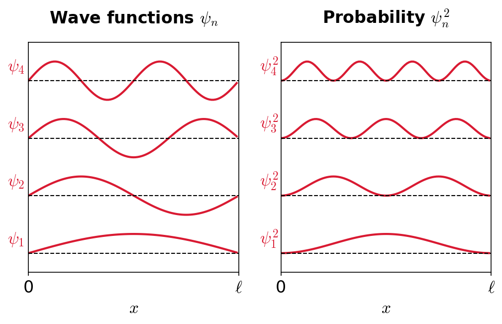
The probability of observing the particle between \(x\) and \(x+dx\) in each state is \(P_n\ dx \propto |\psi_n(x)|^2 dx\). Notice that \(E_o = 0\) is not a possible state, where the lowest energy level is \(E_1\) with a probability density \(P_1 \propto |\psi_1(x)|^2\). *The most probable location for the particle in the lowest energy state is in the middle of the box.
The particle-in-a-box model is our first application of quantum mechanics. The quantization of energy arises from the need to fit a whole number of half-waves into the box. The concept of energy levels (as first discussed in the Bohr model) arose in a natural way by using waves.
Exercise 5.9
Find first three quantized energy levels of an electron constrained to move in a one-dimensional atom of size \(0.1\ {\rm nm}\).
The particle-in-a-box model can be used for a constrained electron, where we know the energy levels are
The first three energy levels are \(E_1 = 38\ {\rm eV}\), \(E_2 = 150\ {\rm eV}\), and \(E_3 = 338\ {\rm eV}\).
from scipy.constants import h,m_e,eV

def PIB_En(n,m,ell):
    #Calculate the energy levels for a particle-in-a-box
    #n = integer
    #m = mass of particle (in kg)
    #ell = width of box (in m)
    return n**2*h**2/(8*m*ell**2)

ell_e = 1e-10 #size of box in m
for i in range(1,4):
    E_n = PIB_En(i,m_e,ell_e)
    print("The E_%i energy is %1.2e J or %i eV.\n" % (i,E_n,np.round(E_n/eV,0)))
The E_1 energy is 6.02e-18 J or 38 eV.

The E_2 energy is 2.41e-17 J or 150 eV.

The E_3 energy is 5.42e-17 J or 338 eV.
5.9. Homework Problems#
Problem 1
X rays scattered from a crystal have a first-order diffraction peak at \(\theta = 12.5^\circ\). At what angle will the second- and third-order peaks appear?
Problem 2
Calculate the de Broglie wavelength of a \(1.2\ \rm kg\) rock thrown with a speed of \(6.0\ \rm m/s\) into a pond. Is this wavelength similar to that of the water waves produced? Explain.
Problem 3
In an electron-scattering experiment, an intense reflected beam is found at \(\phi =32^\circ\) for a crystal with an interatomic distance of \(0.23\ \rm nm\). What is the lattice spacing of the planes responsible for the scattering? Assuming first-order diffraction, what are the wavelength momentum, kinetic energy, and total energy of the incident electron?
Problem 4
Two waves are traveling simultaneously down a long Slinky. They can be represented by
where the amplitudes are in meters and time is in seconds.
a. Write the expression for the resulting wave.
b. What are the phase and group velocities?
c. What is \(\Delta x\) between two adjacent zeros of \(\Psi\)?
d. What is \(\Delta k\ \Delta x\)?
Problem 5
Light of intensity \(I_o\) passes through two sets of apparatus. One contains one slit and the other two slits. The slits have the same width. What is the ratio of the outgoing intensity amplitude for the central peak for the two slit case compared to the single slit?
Problem 6
A neutron is confined in a deuteron of diameter \(3.1 \times 10^{-15}\ \rm m\). Use the energy level calculation of a one-dimensional box to calculate the neutron’s minimum kinetic energy. What is the neutron’s minimum kinetic energy according to the uncertainty principle?
Problem 7
The wave function of a particle in a one-dimensional box of width \(L\) is \(\psi(x) = A\sin(\pi x/L)\). If we know that the particle must be somewhere in the box, what must be the value of A?
Problem 8
Write down the normalized wave function for the first three energy levels of a particle of mass \(m\) in a one-dimensional box of width \(L\). Assume there are equal probabilities of being in each state.