7. The Hydrogen Atom and Atomic Physics

The hydrogen atom is the simplest, containing a single electron and proton, and has been the object of more experimentation (and study) than any other atom. The hydrogen atom has been studied using the Bohr model to better predict spectral absorption and emission lines. We can now apply the Schrödinger equation to the hydrogen atom and further develop quantum mechanics using a real system. This requires a statistical interpretation of nature (at least for the very small) and the use of quantum numbers that are needed to explain experimental results.

7.1. Application of the Schrödinger Equation to the Hydrogen Atom

The hydrogen atom requires the full complexity of the 3D Schrödinger equation, which requires a description of the potential energy in a 3D coordinate system. To a good approximation, the potential energy of the hydrogen atom is simply electrostatic:

(7.1)\[V(r) = -\frac{e^2}{4\pi \epsilon_o r}.\]

The 3D time-independent Schrödinger equation can be written as

(7.2)\[\begin{split}-\frac{\hbar^2}{2m}\nabla^2\psi + V\psi &= E\psi, \\ -\frac{\hbar^2}{2\mu}\left[\frac{1}{r^2} \frac{\partial}{\partial r}\left(r^2 \frac{\partial \psi}{\partial r}\right) + \frac{1}{r^2\sin \theta}\frac{\partial}{\partial \theta}\left( \sin \theta \frac{\partial \psi}{\partial \theta} \right) + \frac{1}{r^2\sin^2 \theta}\frac{\partial^2 \psi}{\partial \phi^2} \right] + V\psi &= E\psi,\end{split}\]

where the first equation is a general form and the second equation is written using spherical polar coordinates \((r,\ \theta,\ \phi)\) using the reduced mass \(\mu\). In the terminology of partial differential equations, Equation (7.2) is separable, which means that a solution may be determined using the product of three functions that depend only on one of the respective coordinates. Thus, a trial solution is written as

(7.3)\[\psi\left(r,\ \theta,\ \phi \right) = R(r)f(\theta)g(\phi).\]

From Section 6.5, we known that the solution will have at least one quantum number. In fact, we should expect there to be a quantum number corresponding to each dimension of motion.

7.2. Solution of the Schrödinger Equation for the Hydrogen Atom

The first step in solving the Schrödinger equation for the Hydrogen Atom is to substitute the trial solution (Eq. (7.3)) into Eq. (7.2). Then we can separate the resulting equation into three equations that correspond to the respective functions of each dimension. The solutions to those equations will then provide a better understanding for the structure of the hydrogen atom, in both the ground state and in the excited states.

7.2.1. Separation of Variables

Starting with Eq. (7.3), we find the necessary derivatives as

(7.4)\[\frac{\partial \psi}{\partial r} = fg\frac{\partial R}{\partial r}, \qquad \frac{\partial \psi}{\partial \theta} = Rg\frac{\partial f}{\partial \theta}, \qquad \text{and}\quad \frac{\partial^2 \psi}{\partial \phi^2} = Rf\frac{\partial^2 g}{\partial \phi^2}.\]

We substitute substitute these results into Eq. (7.2) to get

(7.5)\[\begin{align} -\frac{\hbar^2}{2\mu}\left[\frac{fg}{r^2} \frac{\partial}{\partial r}\left(r^2 \frac{\partial R}{\partial r}\right) + \frac{Rg}{r^2\sin \theta}\frac{\partial}{\partial \theta}\left( \sin \theta \frac{\partial f}{\partial \theta} \right) + \frac{Rf}{r^2\sin^2 \theta}\frac{\partial^2 g}{\partial \phi^2} \right] + V(Rfg) &= E(Rfg). \end{align}\]

Next we multiply both sides by \(r^2 \sin^2 \theta/ (Rfg)\) and rearrange to have

(7.6)\[-\left[\frac{\sin^2 \theta}{R} \frac{\partial}{\partial r}\left(r^2 \frac{\partial R}{\partial r}\right) + \frac{\sin \theta}{f}\frac{\partial}{\partial \theta}\left( \sin \theta \frac{\partial f}{\partial \theta} \right) \right] - \frac{2\mu}{\hbar^2}(E-V)r^2 \sin^2 \theta = \frac{1}{g}\frac{\partial^2 g}{\partial \phi^2}\]

Equation (7.6) shows that only the variables \(r\) and \(\theta\) (and their respective functions) appear on the left side, and the azimuthal variable \(\phi\) (and its function \(g\)) is separated onto the right side. What does this mean? The left side of the equation cannot change as \(\phi\) changes because it does not have any variables (or functions) that depend on \(\phi\). It then follows that the right side doesn’t change with \(r\) or \(\theta\). Both sides of the equation have to equal the same thing, and we set that as a constant \(-m_\ell^2\). Then the right hand side can become (after some rearranging)

(7.7)\[\frac{d^2 g}{d\phi^2} = -m_\ell^2.\]

The partial derivatives \(\partial\) can be changed to ordinary derivatives \(d\) because the function \(g\) depends only on a single variable \(\phi\). Equation (7.7) is called the azimuthal equation as it describes changes in the azimuth angle (defined in astronomy). The differential equation is that of a harmonic oscillator, which has solutions in terms of sines and cosines. But, we find it convenient to choose a more compact form in terms of exponential functions \(e^{im_\ell \phi}\). The value \(m_\ell\) represents an integer (either positive or negative) or zero.

Returning to left hand side of Eq. (7.6), we can write (after some rearranging)

(7.8)\[\frac{1}{R} \frac{\partial}{\partial r}\left(r^2 \frac{\partial R}{\partial r}\right) + \frac{2\mu r^2}{\hbar^2}(E-V) = \frac{m_\ell^2}{\sin^2 \theta} - \frac{1}{f\sin \theta}\frac{\partial}{\partial \theta}\left( \sin \theta \frac{\partial f}{\partial \theta} \right).\]

Equation (7.8) is separated with the radial terms on the left side and the angular terms on the right. Using a similar procedure as before, we set both sides equal to a constant, we call \(\ell(\ell+1)\). Doing so results in the following equations:

(7.9)\[\frac{1}{r^2} \frac{d}{d r}\left(r^2 \frac{d R}{d r}\right) + \frac{2\mu}{\hbar^2}\left[E-V - \frac{\hbar^2}{2\mu}\frac{\ell(\ell+1)}{r^2}\right]R = 0, \qquad \text{Radial equation}\]

and

(7.10)\[\frac{1}{\sin \theta}\frac{d}{d \theta}\left( \sin \theta \frac{d f}{d \theta} \right) + \left[\ell(\ell+1) - \frac{m_\ell^2}{\sin^2 \theta}\right]f = 0. \qquad \text{Angular equation}\]

Similar to the azimuthal equation, we replace the partial derivatives with ordinary ones. The process for separation of variables is complete, where the Schrödinger equation for the hydrogen atom is represented by three ordinary differential equations, each containing a single variable.

7.2.2. Solution of the Radial Equation

The radial equation (Eq. (7.9)) has well known solutions because it is very similar (with some rearranging) to the Laguerre equation developed by Edmond Laguerre. The solutions to the radial equation will define a radially dependent function \(R\) that satisfy the appropriate boundary conditions and take the form of the associated Laguerre polynomials.

Let’s first look at the ground state wave function \(n=0\), which will necessarily describe the lowest possible angular momentum quantum number \(\ell = 0\) of the system. When \(\ell = 0\), Eq. (7.9) simplifies to:

(7.11)\[\begin{split}\frac{1}{r^2} \frac{d}{d r}\left(r^2 \frac{d R}{d r}\right) + \frac{2\mu}{\hbar^2}\left[E-V\right]R &= 0, \\ \frac{d^2 R}{d r^2} + \frac{2}{r}\frac{d R}{d r} + \frac{2\mu}{\hbar^2}\left[E-V\right]R &= 0.\end{split}\]

We can then replace \(V\) with the Coulomb potential energy (Eq. (7.1)) to find

(7.12)\[\frac{d^2 R}{d r^2} + \frac{2}{r}\frac{d R}{d r} + \frac{2\mu}{\hbar^2}\left[E+\frac{e^2}{4\pi \epsilon_o r}\right]R = 0.\]

Similar to the solution for the azimuthal equation, we will try a solution with an exponential. With some prior experience in solving differential equations, we try a solution having the form

(7.13)\[\begin{align} R = Ae^{-r/a_o}, \end{align}\]

where \(A\) is a normalization constant and \(a_o\) is a constant that must cancel out the dimension of \(r\) with a length. The first and second derivatives are

(7.14)\[\begin{align} \frac{dR}{dr} = -\frac{A}{a_o}e^{-r/a_o} = -\frac{R}{a_o}, \qquad \text{and} \qquad \frac{d^2R}{dr^2} = \frac{R}{a_o^2}. \end{align}\]

Substituting these derivatives into Eq. (7.12) yields

(7.15)\[\begin{split}\frac{R}{a_o^2} - \frac{2R}{ra_o} + \frac{2\mu}{\hbar^2}\left[E+\frac{e^2}{4\pi \epsilon_o r}\right]R &= 0, \\ \left(\frac{2\mu e^2}{4\pi \epsilon_o \hbar^2} - \frac{2}{a_o}\right)\frac{1}{r} + \left(\frac{1}{a_o^2} + \frac{2\mu E}{\hbar^2}\right) & = 0.\end{split}\]

Trying to solve Eq. (7.15) for \(r\) algebraically is rather complicated, where we’ll use the more trivial solution that each of the terms in parentheses are themselves equal to zero. By setting the first term in parentheses to zero and solving for \(a_o\), we find

(7.16)\[\begin{align} a_o = \frac{4\pi \epsilon_o \hbar^2}{\mu e^2}, \end{align}\]

and that \(a_o\) is equal to the Bohr radius (see Sect. 4.4). Then we can set the second term in parentheses to zero and solve for \(E\) to find

(7.17)\[\begin{align} E = -\frac{\hbar^2}{2\mu a_o^2} = -E_o, \end{align}\]

which is the ground state energy from the Bohr model.

Introduction to Quantum Numbers The full solution to the radial equation introduces the quantum number n, which is a positive (non-zero) integer. The angular equation (Eq. (7.10)) is similar to a mathematical equation solved by Adrien-Marie Legendre who found solutions to the differential equation long before the quantum mechanical description of the hydrogen atom. Therefore the angular equation will have solutions related to Legendre polynomials. Application of the appropriate boundary conditions leads to particular restrictions on the quantum numbers \(\ell\) and \(m_\ell\):

(7.18)\[\begin{split}\ell &= 0,\ 1,\ 2,\ 3,\ \ldots \\ m_\ell &= -\ell,\ (-\ell+1),\ (-\ell+2),\ \ldots,\ -1,\ 0,\ 1,\ (\ell+2),\ (\ell+1),\ \ell.\end{split}\]

The quantum number \(\ell\) must be a positive integer (including zero), and the quantum number \(m_\ell\) must be an integer subject to the restriction that \(|m_\ell| \leq \ell\). There is a further restriction on the quantum number \(\ell\), such that \(\ell < n\). The first few radial wave functions \(R_{n\ell}\) are listed in Table 7.1.

Table 7.1 Hydrogen Atom Radial Wave Functions

\(n\)	\(\ell\)	\(R_{n\ell}(r)\)
1	0	\(2 \frac{e^{-r/a_o}}{a_o^{3/2}}\)
2	0	\(\left(2-\frac{r}{a_o}\right) \frac{e^{-r/(2a_o)}}{2a_o^{3/2}}\)
2	1	\(\frac{r}{a_o}\frac{e^{-r/(2a_o)}}{\sqrt{3}(2a_o)^{3/2}}\)
3	0	\(\frac{2}{81}\left(27-18\frac{r}{a_o} + 2 \frac{r^2}{a_o^2} \right)\frac{e^{-r/(3a_o)}}{\sqrt{3}a_o^{3/2}}\)
3	1	\(\frac{4}{81}\left(6\frac{r}{a_o} - \frac{r^2}{a_o^2} \right)\frac{e^{-r/(3a_o)}}{\sqrt{6}a_o^{3/2}}\)
3	2	\(\frac{4}{81}\frac{r^2}{a_o^2}\frac{e^{-r/(3a_o)}}{\sqrt{30}a_o^{3/2}}\)

7.2.3. Solution of the Angular and Azimuthal Equations

In the azimuthal equation, its solution can be expressed in exponential form, but the angular equation also contains the quantum number \(m_\ell\). Thus the solutions to the angular and azimuthal equations are linked. It is customary to group these solution together into so-called spherical harmonics defined as

(7.19)\[\begin{align} Y(\theta,\ \phi) = f(\theta)g(\phi), \end{align}\]

where the \(f(\theta)\) is a Legendre polynomial of order \(\ell\). See Table 7.2 for a listing of the normalized spherical harmonics up to \(\ell = 3\).

Table 7.2 Normalized Spherical Harmonics \(Y(\theta,\ \phi)\)

\(\ell\)	\(m_\ell\)	\(Y_{\ell m_\ell}(r)\)
0	0	\(\frac{1}{\sqrt{4\pi}}\)
1	0	\(\sqrt{\frac{3}{4\pi}}\cos \theta\)
1	\(\pm 1\)	\(\mp\sqrt{\frac{3}{8\pi}}\sin \theta e^{\pm i\phi}\)
2	0	\(\sqrt{\frac{5}{16\pi}}\left(3\cos^2 \theta - 1 \right)\)
2	\(\pm 1\)	\(\mp\sqrt{\frac{15}{8\pi}}\sin \theta \cos \theta e^{\pm i\phi}\)
2	\(\pm 2\)	\(\sqrt{\frac{15}{32\pi}}\sin^2 \theta \cos \theta e^{\pm 2i\phi}\)
3	0	\(\sqrt{\frac{7}{16\pi}}\left(5\cos^3 \theta - 3 \cos \theta\right)\)
3	\(\pm 1\)	\(\mp \sqrt{\frac{21}{64\pi}}\sin \theta \left(5\cos^2 \theta - 1\right)e^{\pm i\phi}\)
3	\(\pm 2\)	\(\sqrt{\frac{105}{32\pi}}\sin^2 \theta \cos \theta e^{\pm 2i\phi}\)
3	\(\pm 3\)	\(\mp \sqrt{\frac{35}{64\pi}}\sin^3 \theta e^{\pm 3i\phi}\)

Exercise 7.1

Show that the spherical harmonic function \(Y_{11}(\theta,\ \phi)\) satisfies the angular equation (Eq. (7.10)).

From the spherical harmonic function \(Y_{11}(\theta,\ \phi)\) , we deduce that \(\ell = 1\) and \(m_\ell = 1\) from the subscript. To simplify our calculation we rewrite \(Y_{11}(\theta,\ \phi)\) as

\[ Y_{11}(\theta,\ \phi) = -\sqrt{\frac{3}{8\pi}}\sin \theta e^{\pm i\phi} = A \sin \theta. \]

Note that we chose the minus value from Table 7.2 because \(m_\ell\) is positive. The factor \(A\) includes all the constants and the exponential term \(e^{i\phi}\). Now we insert this function into the angular equation (Eq. (7.10)), where we have

\[ \frac{1}{\sin \theta} \frac{d}{d\theta}\left[A\sin \theta \frac{d(\sin \theta)}{d\theta} \right] + \left(2 - \frac{1}{\sin^2 \theta}\right) A \sin \theta = 0. \]

Since \(A\) is common to both terms we can divide it through and discard it. Then we’re left with calculating the derivative as

\[\begin{align*} \frac{1}{\sin \theta} \frac{d}{d\theta}\left[\sin \theta \cos \theta \right] + 2 \sin \theta - \frac{1}{\sin \theta} &= 0, \\ \frac{1}{\sin \theta} \left(\cos^2 \theta - \sin^2 \theta \right) + 2 \sin \theta - \frac{1}{\sin \theta} &= 0, \\ \frac{1}{\sin \theta} - 2\sin \theta + 2 \sin \theta - \frac{1}{\sin \theta} &= 0, \\ 0 &= 0. \end{align*}\]

Thus Eq. (7.10) is satisfied by the spherical harmonic function \(Y_{11}(\theta,\ \phi)\).

Exercise 7.2

Show that the hydrogen wave function \(\psi_{211}\) is normalized.

A normalized function (e.g., \(\psi_{n\ell m_\ell}\)) has an area under the curve equal to unity, which is given mathematically as

(7.20)\[\begin{align} 1 &= \int \psi^*_{n\ell m_\ell} \psi_{n\ell m_\ell} d\tau, \\ & = \int \psi^*_{211} \psi_{211} r^2 \sin \theta\ dr\ d\theta\ d\phi, \end{align}\]

where \(d\tau = r^2 \sin \theta\ dr\ d\theta\ d\phi\) is the volume element in spherical coordinates. We construct the wave function \(\psi_{211}\) using the respective functions from Tables 7.1 and 7.2.

\[\begin{align*} \psi_{211} &= R_{21}Y_{11}, \\ &= \left[ \frac{r}{a_o}\frac{e^{-r/(2a_o)}}{\sqrt{3}(2a_o)^{3/2}}\right] \left[-\sqrt{\frac{3}{8\pi}}\sin \theta e^{i\phi}\right]. \end{align*}\]

To evaluate the normalization integral, we need to compute the product of the wave function \(\psi_{211}\) with its complex conjugate \(\psi^*_{211}\). This is given as:

\[\begin{align*} \psi^*_{211} \psi_{211} &= \left[ \frac{r}{a_o}\frac{e^{-r/(2a_o)}}{\sqrt{3}(2a_o)^{3/2}}\right] \left[-\sqrt{\frac{3}{8\pi}}\sin \theta e^{-i\phi}\right]\left[ \frac{r}{a_o}\frac{e^{-r/(2a_o)}}{\sqrt{3}(2a_o)^{3/2}}\right] \left[-\sqrt{\frac{3}{8\pi}}\sin \theta e^{i\phi}\right], \\ & = \left[ \frac{r^2}{24a^5_o}e^{-r/a_o}\right] \left[\frac{3}{8\pi}\sin^2 \theta \right], \\ & = \frac{r^2}{64 \pi a^5_o}e^{-r/a_o} \sin^2 \theta. \end{align*}\]

Inserting into the normalization integral produces:

\[\begin{align*} \int \psi^*_{211} \psi_{211} r^2 \sin \theta\ dr\ d\theta\ d\phi & = \int \frac{r^2}{64 \pi a^5_o}e^{-r/a_o} \sin^2 \theta\ r^2 \sin \theta\ dr\ d\theta\ d\phi, \\ & = \frac{1}{64 \pi a^5_o} \int_{0}^{\infty} r^4 e^{-r/a_o} dr \int_0^\pi \sin^3 \theta\ d\theta\ \int_0^{2\pi} d\phi, \\ & = \frac{1}{64 \pi a^5_o} \left[ 24a_o^5 \right] \left[ \frac{4}{3}\right] \left[2\pi \right], \\ & = 1. \end{align*}\]

The wave function is indeed normalized.

7.3. Quantum Numbers

Three quantum numbers are introduced when solving Eq. (7.2), which are:

• \(n\) Principal quantum number,

• \(\ell\) Orbital angular momentum quantum number, and

• \(m_\ell\) Magnetic quantum number.

The values of the quantum numbers are obtained by applying boundary conditions to the wave function \(\psi\). The boundary conditions require that the wave function have acceptable properties (e.g., single-valued and finite). The restriction for \(n\) is that it is an positive (non-zero) integer, where the restrictions for \(\ell\) and \(m_\ell\) are given in Eq. (7.18).

Additionally, the orbital angular momentum quantum number \(\ell\) must be less than than the principe quantum number (i.e., \(\ell < n\)). The magnitude of the magnetic quantum number \(m_\ell\) must be less than or equal to the orbital angular momentum quantum number (i.e., \(|m_\ell| \leq \ell\)).

Exercise 7.3

What are the possible quantum numbers for the state n = 4 in atomic hydrogen?

We want to apply the restrictions for the quantum numbers, which is best shown through a table.

Table 7.3 Quantum Numbers for \(n=4\) in Atomic Hydrogen

\(\mathbf{n}\)	\(\mathbf{\ell}\)	\(\mathbf{m_\ell}\)
4	0	0
4	1	-1, 0, 1
4	2	-2, -1, 0, 1, 2
4	3	-3, -2, -1, 0, 1, 2, 3

Quantum numbers are generated for \(\ell < 4\), but not \(\ell = 4\).

7.3.1. Principal Quantum Number \(n\)

The principal quantum number \(n\) results from the solution of the radial equation (Eq. (7.9)). The radial equation includes the potential energy \(V(r)\), where the boundary conditions on \(R(r)\) quantize the energy \(E\) and is equal to the value found in the Bohr model.

The energy levels (so far) depend on only on the principal quantum number \(n\). The energies are negative, which indicates that the electron and proton are bound together (i.e., the electron lies within an electrostatic well produced by the proton).

It is perhaps surprising that the total energy of the electron does not depend on the angular momentum. However, a similar result appears in the solution for planetary motion. A planet’s energy depends solely on the semimajor axis and not on its orbital eccentricity. This occurs because the gravitational and electrostatic forces act from central bodies and the force laws have an inverse-square dependence on distance.

7.3.2. Orbital Angular Momentum Quantum Number \(\ell\)

The orbital angular momentum quantum number \(\ell\) arises in both the radial and angular (Eq. (7.10)) equations of the wave function. The electron-proton system has orbital angular momentum from the relative motion of both particles. Classically, the angular momentum is given as

\[ \vec{L} = \vec{r} \times \vec{p},\]

with a magnitude \(L = mv_{\rm orb}r\) and the \(v_{\rm orb}\) represents the electron’s orbital velocity perpendicular to its orbital radius \(r\). The quantum number \(\ell\) is related to the magnitude of the orbital angular momentum number \(L\) by,

(7.21)\[\begin{align} L = \sqrt{\ell(\ell + 1)}\hbar. \end{align}\]

The dependence on \(\ell(\ell + 1)\) is a wave phenomenon that results from applying the boundary conditions on \(\psi\). The quantum result disagrees with the Bohr’s theory, where \(L = n\hbar\). This will force us to discard Bohr’s semiclassical “planetary” model when considering the finer structures of the atom.

An energy level is degenerate with respect to \(\ell\) when the energy is independent of the value of \(\ell\). For example for an \(n= 3\) state, the energy is the same for all possible values of \(\ell\) (i.e., \(\ell = 0,\ 1,\ 2\)). It is customary (especially in chemistry) to use letter names for the various \(\ell\) values. These are

\[\begin{align*} \ell &=& &0& &1& &2& &3& &4& 5\ldots \\ \text{Letter} &=& &s& &p& &d& &f& &g& h\ldots \end{align*}\]

The choices for the first 4 letter designations originate from visual observations of early spectra that were sharp, principal, diffuse, and fundamental. After \(\ell = 3\), the letters follow alphabetical order.

Atomic states are usually referred by their \(n\) and \(\ell\) combination with the number and letter. For example, a state with \(n=2\) and \(\ell = 1\) is called the \(2p\) state.

7.3.3. Magnetic Quantum Number \(m_\ell\)

The orbital angular momentum quantum number \(\ell\) determines the magnitude of the angular momentum \(\vec{L}\), but \(\vec{L}\) is a vector which has a direction. Classically, there is

• no torque in the hydrogen atom in the absence of external fields,

• a constant of the motion through the angular momentum, and

• conservation of angular momentum.

The solution to the Schrödinger equation for the angular equation \(f(\theta)\) specifies that \(\ell\) is an integer, and therefor the magnitude of \(\vec{L}\) is quantized.

The azimuthal angle \(\phi\) measures a rotation about the \(z\)-axis. The solution of the azimuthal equation \(g(\phi)\) specifies that \(m_\ell\) is an integer and is related to \(L_z\) (i.e., the \(z\)-component of the angular momentum) by

(7.22)\[\begin{align} L_z = m_\ell \hbar. \end{align}\]

The relationship of \(L,\ L_z,\ \ell,\) and \(m_\ell\) is displayed in Fig. 7.1 for the value \(\ell=2\). Because \(L_z\) is quantized, only certain orientations of \(\vec{L}\) are possible and each orientation corresponds to a different \(m_\ell\). This phenomenon is called space quantization because only certain orientations of \(\vec{L}\) are allowed in space.

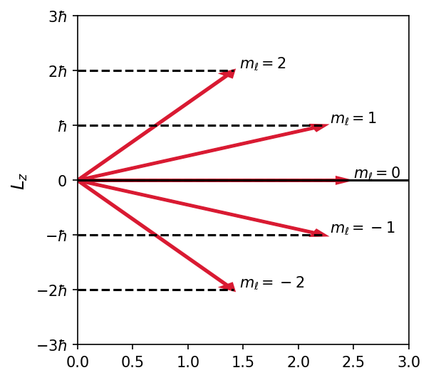
Fig. 7.1 Schematic diagram of the relationship between \(\vec{L}\) and \(L_z\), with the allowed values of \(m_\ell\). The length of each vector is equal to the magnitude of \(L\).

import numpy as np
import matplotlib.pyplot as plt 
from myst_nb import glue

ell = 2.
arrow_len = np.sqrt(ell*(ell+1.)) #in units of hbar; L/hbar = \sqrt(ell(ell+1))

ylabels = ['$-3\hbar$','$-2\hbar$','$-\hbar$','0','$\hbar$','$2\hbar$','$3\hbar$']
col = (218/256., 26/256., 50/256.)
aw = 0.01
hw = 10*aw
hl = hw
fs = 'large'

fig = plt.figure(figsize=(4,4),dpi=150)
ax = fig.add_subplot(111)
ax.axhline(0,0,1,color='k')
for m_idx in range(0,5):
    dy = 2 - m_idx
    dx = np.sqrt(arrow_len**2-dy**2)
    ax.axhline(2-m_idx,0,np.abs(dx)/3,color='k',linestyle='--')
    ax.arrow(0,0,dx,dy,lw=2,width=aw,head_width=hw,head_length=hl,length_includes_head=True,color=col)
    ax.text(dx+0.05,dy+0.05,'$m_\ell = %i$' % dy)
    

ax.set_xlim(0,3)
ax.set_ylim(-3,3)
ax.set_yticks(np.arange(-3,4,1))
ax.set_yticklabels(ylabels)
ax.set_ylabel("$L_z$",fontsize=fs)

glue("Lz_fig", fig, display=False);

Where is the \(z\)-axis in space? The choice of the \(z\)-axis is completely arbitrary unless there is an external magnetic field. It is customary to choose the \(z\)-axis to be along the \(\vec{B}\) if there is a magnetic field, which is why \(m_\ell\) is called the magnetic quantum number.

Will the angular momentum be quantized along the \(x\)- and \(y\)-axes as well? Quantum mechanics allows \(\vec{L}\) to be quantized along only one direction in space. Through the magnitude of \(\vec{L}\) and \(L_z\), we have some constraints on \(L_x\) and \(L_y\) from the relation \(L^2 = L_x^2 + L_y^2 + L_z^2\). Consider the following argument:

• If all three components of \(\vec{L}\) were known, then the direction of \(\vec{L}\) would also be known.

• In this case we would have a precise knowledge of one component of the electron’s position in space because the electron’s orbital motion is confined to a plane perpendicular to \(\vec{L}\).

• Confinement of the electron to that plane means that the electron’s momentum component along \(\vec{L}\) is exactly zero.

The simultaneous knowledge of the same component of position and momentum is forbidden by the uncertainty principle.

Only the magnitude of \(\vec{L}\) and \(L_z\) may be specified simultaneously. The values of \(L_x\) and \(L_y\) must be consistent with \(L^2 = L_x^2 + L_y^2 + L_z^2\) but cannot be specified individually. The angular momentum vector \(\vec{L}\) never points in the \(z\) direction because \(L = \sqrt{\ell(\ell _ 1)}\hbar\) and \(L > L_z^{\rm max} = \ell \hbar\).

The values of \(L_z\) range from \(-\ell\) to \(\ell\) in steps of \(1\), for a total of \(2\ell + 1\) allowed values. There is nothing special about the Cartesian directions, and thus we expect the average angular momentum components squared in the three directions to be the same (i.e., \(\langle L_x^2\rangle = \langle L_y^2\rangle = \langle L_z^2\rangle\)). the average value of \(\langle L^2 \rangle\) is equal to three times the average value of any one of the components. To find \(\langle L^2 \rangle\), we use \(L_z\) to get

(7.23)\[\begin{align} \langle L^2 \rangle &= 3 \langle L_z^2 \rangle = \frac{3}{2\ell + 1} \sum_{m_\ell = - \ell}^\ell (m_\ell \hbar)^2, \\ & = \frac{3}{2\ell + 1} \left[\frac{\ell}{3}(\ell+1)(2\ell+1)\hbar^2\right], \\ &= \ell(\ell+1)\hbar^2. \end{align}\]

The summation can be evaluated with the help of a list of mathematical series.

Exercise 7.4

What is the degeneracy of the \(n=3\) level?

To find the total degeneracy for \(n=3\), we have to add all the possibilities.

Table 7.4 Quantum Numbers for \(n=3\) in Atomic Hydrogen

\(\mathbf{n}\)	\(\mathbf{\ell}\)	\(\mathbf{m_\ell}\)	\(\mathbf{2\ell + 1}\)
3	0	0	1
3	1	-1, 0, 1	3
3	2	-2, -1, 0, 1, 2	5

For each value of \(\ell\) there are \(2\ell + 1\) states. From Table 7.4, we can add the values from the \(2\ell +1\) column for a total of \(9\) states. All nine states have the same energy, but different quantum numbers.

7.4. Magnetic Effects on Atomic Spectra - The Normal Zeeman Effect

In 1896, Pieter Zeeman showed that the spectral lines emitted by atoms placed in a magnetic field are broadened and split. The splitting of an energy level into multiple levels in the presences of an external magnetic field is called the Zeeman effect. There are two forms of the Zeeman effect:

• the normal Zeeman effect occurs when a spectral line is split into three lines.

• the anomalous Zeeman effect is when a spectral line is split into more than three lines.

The normal Zeeman effect can be explained by considering the atom to behave like a small magnet. By the 1920s, the fine structure of atomic spectral lines from hydrogen and other elements had already been identified. Fine structure refers to the splitting of a spectral line into more closely spaced lines.

As a rough model, think of an electron circulating around the nucleus as a circular current loop. The current loop has a magnetic moment \(\mu = IA\), which depends on the area of the current loop \(A\) and the movement of the electron through a current \(I = dq/dt\). The current can be calculated as the electron charge \(-e\) divided by the period \(T\) to make one revolution $T = 2\pi r/v). Thus the magnetic moment is:

(7.24)\[\begin{align} \mu &= IA = \frac{q}{T}A, \\ &= -\frac{e\pi r^2}{2\pi r/v},\\ & = -\frac{1}{2}erv, \\ & = -\frac{eL}{2m}, \end{align}\]

and can be written in terms of the orbital angular momentum \(L = mvr\). Both the magnetic moment \(\vec{\mu}\) and angular momentum \(\vec{L}\) are vectors so that

(7.25)\[\begin{align} \vec{\mu} = -\frac{e}{2m}\vec{L}. \end{align}\]

In the absence of an external magnetic field to align them, the magnetic moments \(\vec{\mu}\) of atoms point in random directions. In classical electromagnetism, if a magnetic dipole is placed in an external field, then the dipole will experience a torque \(\vec{\tau} = \vec{\mu} \times \vec{B}\) that tends to align the dipole with the magnetic field. The dipole has a potential energy \(V_B\) in the field given by

(7.26)\[\begin{align} V_B = -\vec{\mu} \cdot \vec{B}. \end{align}\]

According to classical physics, the magnetic moment will align itself with the external magnetic field to minimize energy as long as the system can change its potential energy.

Note

There is a similarity to the case of a spinning top in a gravitational field. A child’s spinning top precesses about the gravitational field, where the spin axis rotates about the direction of the gravitational force. (i.e., vertical). The gravitational field is not parallel to the angular momentum, and the force of gravity results in a precession of the top about the field direction.

The angular momentum is aligned with the magnetic moment, and the torque (due to the magnetic moment) causes a precession of \(\vec{\mu}\) about the magnetic field, not an alignment. The magnetic field establishes a preferred direction in space along which we customarily define the \(z\)-axis. Then we have

(7.27)\[\begin{align} \mu_z = \frac{e\hbar}{2m}m_\ell = -\mu_B m_\ell, \end{align}\]

where a unit of the magnetic moment \(\mu_B\) is called the Bohr magneton. From the quantization of \(L_z\) and that \(L>m_\ell \hbar\), we cannot have \(|\vec{\mu}| = \mu_z\), or the magnetic moment can’t align itself exactly in the \(z\)-direction. Therefore, the magnetic moment has only certain quantized orientations.

What about the energy of the orbiting electron in a magnetic field? For the magnetic moment to rotate away from the magnetic field \(\vec{B}\), it takes work. Assuming the \(\vec{B}\) is oriented along the \(z\) direction, the potential energy due to the magnetic field is given by

(7.28)\[V_B = -\mu_z B = \mu_B m_\ell B.\]

The potential energy is quantized according to the magnetic quantum number \(m_\ell\). Each (degenerate) atomic level of a given \(\ell\) is split into \(2\ell + 1\) different energy states depending on the the value of \(m_\ell\). The energy degeneracy of a given \(n\ell\) level is removed by a magnetic field. If the degenerate energy of a state is given by \(E_o\), then the three different energies in a magnetic field \(B\) for a \(\ell = 1\) state are:

Table 7.5 Energy states for \(\ell = 1\) due to a magnetic field $\vec{B}.

\(m_\ell\)	Energy
1	\(E_o + \mu_B B\)
0	\(E_o\)
\(-1\)	\(E_o - \mu_B B\)

The splitting of spectral lines (i.e., the normal Zeeman effect) can be partially explained by the application of external magnetic fields. When a magnetic field is applied, the \(2p\) (\(\ell = 1\)) level of atomic hydrogen is split into three different states. The energy differences between the states are quite small.

In the 1920s, physicists tried to detect the effects of space quantization (\(m_\ell\)) by measuring the energy difference \(\Delta E\) between the split energy states. In 1922, Otto Stern and Walther Gerlach reported the results of an experiment that clearly showed evidence for space quantization (i.e., Stern-Gerlach Experiment).

If an external magnetic field is inhomogenous (e.g., stronger at the south pole than at the north pole), then there will be a net force and torqure on a magnet placed in the field. By passing an atomic beam of particles in teh \(\ell = 1 \) state through a magnetic field along the \(z\) direction, there is a potential energy \(V_B = -\mu_z B\). The force on the particles is \(F_z = -(dV_B/dz) = \mu_z(dB/dz)\). The \(m_\ell = +1\) state will be deflected down, the \(m_\ell = -1\) will go up, and the $m_\ell = 0 state will be undeflected.

Stern and Gerlach performed their experiment with silver atoms and observed two distinct line instead of three. This was clear evidence for space quantization, although the number of \(m_\ell\) states is always odd.

7.5. Intrinsic Spin

Wolfgang Pauli was the first to suggest that a fourth quantum number assigned to the electron might explain the anomalous optical spectra from the Stern-Gerlach experiment or Zeeman effect. His reasoning was based on relativity, which there are four coordinates and hence, should be four quantum numbers.

In 1925, Samuel Goudsmit and George Uhlenbeck proposed that the electron must have intrinsic angular momentum, and therefore a magnetic moment because the electron is charged. Classically, this corresponds the Earth orbiting the Sun while rotating on its axis. However, this simple classical picture runs into serious difficulties when applied to the spinning charged electron.

Paul Ehrenfest showed that the surface of a spinning electron (or electron cloud) would have to moving at a velocity greater than the speed of light \(c\). If such an intrinsic angular momentum exists, we must regard it as a purely quantum-mechanical result.

To explain the experimental data, Goudsmit and Uhlenbeck proposed that the electron must have an intrinsic spin quantum number \(s= 1/2\). The spinning electron reacts similarly to the orbiting electron in a magnetic field. Therefore, we should try to find quantities analogous to the angular momentum variable \(L\), \(L_z\), \(\ell\), and \(m_\ell\). By analogy, there will be \(2s+1 = 2(1/2) + 1 = 2\) components of the spin angular momentum \(\vec{S}\). Thus the magnetic spin quantum number \(m_s\) has only two values \(m_s = \pm 1/2\). The electron’s spin will be oriented either “up” or “down” in a magnetic field, and the electron can never be spinning with its magnetic moment \(\mu\) exactly along the \(z\) axis (or the direction of the external field \(\vec{B}\)).

Each atomic state is described by three quantum numbers (\(n\), \(\ell\), and \(m_\ell\)) plus an additional quantum number \(m_s \pm 1/2\) that accounts for the spin. The states are degenerate in energy unless an external magnetic field is applied and the energies are split. Then the energy levels introduced by the magnetic field have removed the energy degeneracy.

The intrinsic spin angular momentum vector \(\vec{S}\) has a magnitude \(S = \sqrt{s(s+1)}\hbar\), where the magnetic moment \(\vec{\mu}_s = -(e/m)\vec{S} = -(2\mu_B/hbar)\vec{S}\). Incorporating the special theory of relativity into the Schrödinger equation (i.e., the Dirac equation) introduces a second factor of \(\mu_B\). The relationship between the magnetic moment and the angular momentum vector is called the gyromagnetic ratio and is designated by the letter \(g\), along with an appropriate subscript \(\ell\) or \(s\). In terms of the gyromagnetic ratio:

(7.29)\[\begin{align} \vec{\mu}_\ell &= -\frac{g_\ell \mu_B}{\hbar}\vec{L} &= -\frac{\mu_B}{\hbar}\vec{L} \\ \vec{\mu}_s &= -\frac{g_s \mu_B}{\hbar}\vec{S} &= -\frac{-2\mu_B}{\hbar}\vec{S}. \end{align}\]

The Stern-Gerlach produce two distinct lines due to the quantum number \(m_s\). If the atoms were in a \(\ell = 0\) state, there would be now splitting due to \(m_\ell\), but there is still space quantization due to the intrinsic spin. A similar expression for potential energy from Eq. (7.28) becomes

(7.30)\[\begin{align} V_s = -\vec{\mu} \cdot \vec{B} = \frac{e}{m}\vec{S} \cdot \vec{B}. \end{align}\]

7.6. Energy Levels and Electron Probabilities

A more complete description of the hydrogen includes every possible state with a distinct wave function that is specified by four quantum numbers \(n\), \(\ell\), \(m_\ell\), and \(m_s\). In many cases the energy differences associates with the magnetic numbers \(m_\ell\) and \(m_s\) are insignificant and we can describe the states adequately by \(n\) and \(\ell\) alone.

Generally, capital letters (\(S\), \(P\), and \(D\)) describe the orbital angular momentum of atomic states, while the lower case letters (\(s\), \(p\), and \(d\)) describe the individual electrons. For hydrogen, it makes little difference because each state has only a single electron.

Fig. 7.2 Schematic illustrating the hydrogen energy levels along with the associated electron clouds (shells) due to the spherical harmonics. Image credit: Jeff Cronk @ Gonzaga University)

Figure 7.2 illustrates a diagram that incorporates the energy distinction for \(p\) and \(d\) type orbitals. Such diagrams can be used for hydrogen and many-electron atoms. We have previously learned that atoms emit characteristic electromagnetic radiation when the make transitions to states of lower energy. An atom in its ground state cannot emit radiation because there is not an energy level for which to descend. However, it can absorb EM radiation to gain energy (or through collisions with other atoms), and have one (or more) of its electron transferred to a higher energy state. Then, the atom can emit its characteristic EM radiation.

7.6.1. Selection Rules

7.7. Homework Problems

Problem 1

Assume that the electron in the hydrogen is constrained to move only in a circle of radius \(a\) in the \(x-y\) plane. Show that the separated Schrödinger equation for \(\phi\) becomes

\[\begin{align*} \frac{1}{a^2}\frac{d^2\psi}{d\phi^2} + \frac{2m}{\hbar^2}|E|\psi &= 0, \end{align*}\]

where \(\phi\) describes the phase angle (i.e., position on the circle). Explain why this is similar to the Bohr assumption.

Problem 2

After separating the Schrödinger equation using \(\psi = R(r)f(\theta)g(\phi)\), the equation for \(\phi\) is

\[\begin{align*} -\frac{1}{g}\frac{d^2g}{d\phi^2} &= k^2, \end{align*}\]

where \(k=\text{constant}\). Solve for \(g(\phi)\) in this equation and apply the appropriate boundary conditions. Show that \(k\) must be an integer (including \(0\)) and equal to the magnetic quantum number \(m_\ell\).

Problem 3

Show that the radial wave function \(R_{21}\) for \(n=2\) and \(\ell = 1\) is normalized.

Problem 4

List all the possible quantum numbers \((n,\ \ell,\ m_\ell)\) for the \(n=5\) level in atomic hydrogen.

Problem 5

Calculate the possible \(z\) components of the orbital angular momentum for an electron in a \(3p\) state.

Problem 6

The 21-cm line transition for atomic hydrogen results from a spin-flip transition for the electron in the parallel state of the \(n=1\) state. What temperature in interstellar space gives a hydrogen atom enough energy \((E = 5.9\times 10^{-6}\ \rm eV)\) to excite another hydrogen atom in a collision? (Recall the equation for the \(RMS\) velocity for a gas from Chapter 1)