3. Experimental Quantum Physics

During the 30-year period of 1900-1930, our understanding of physical laws dramatically changed. This was partly motivated by advances in theory by Einstein’s special relativity and through new experimental results (e.g., Michelson-Morley experiment). Another great advance began in 1900 when Max Planck introduced his explanation of blackbody radiation. The discovery of the x-ray, electron, and electron charge were also great experimental achievements.

3.1. Discovery of the X-Ray and the Electron

In the 1890s, cathode rays were easily generated from a metal plate with a large electric potential and in an evacuated tube. However, the origin and constitution of cathode rays was not well understood (or even known). The concept of an atomic substructure of matter was useful to explain the results of chemical experiments, Therefore, physicists deduced that cathode rays had something to do with atoms. For example, cathode rays could penetrate matter, and their properties were of great interest in the 1890s.

In 1895, Wilhelm Röntgen studied how cathode rays interacted with various materials and noticed a phosphorescent screen glowing vividly in the darkened room. Röntgen realized he was observing a new kind of ray that was unaffected by magnetic fields and could better penetrate matter as compared to typical cathode rays. He called them x-rays, where they were apparently produced by the cathode rays bombarding the glass walls of his vacuum tube. Röntgen even showed that he could obtain an image of the bones in a hand when x-rays were allowed to pass through. For his discovery, Röntgen received the first Nobel Prize for Physics in 1901. See the YouTube video below from TedEd for more details.

For several years, before the discovery of x-rays, J.J. Thomson had been studying the properties of electrical discharges in gases. Thomson, Röntgen and many other scientists used a similar apparatus (see Figure 3.1). Thomson believed that cathode rays were particles, whereas several other scientists believed they were wave phenomena.

Fig. 3.1 (a) J. J. Thomson produced a visible beam in a cathode ray tube. (b) This is an early cathode ray tube, invented in 1897 by Ferdinand Braun. (c) In the cathode ray, the beam (shown in yellow) comes from the cathode and is accelerated past the anode toward a fluorescent scale at the end of the tube. Simultaneous deflections by applied electric and magnetic fields permitted Thomson to calculate the mass-to-charge ratio of the particles composing the cathode ray. Image Credit: OpenStax: Chemistry.

Thomson showed in 1897 that the charged particles emitted from a heated electrical cathode were in fact the same as cathode rays. The rays from the cathode are attracted to the positive potential on the anode and further collimated to travel in a straight line, striking a fluorescent screen in the rear of the tube. A voltage across the deflection plates sets up an electric field that deflects charged particles. Thomson also studied the effects of a magnetic field upon the cathode rays and proved convincingly that the cathode rays acted as negatively charged particles (electrons) in both electric and magnetic fields. Thomson received the Nobel Prize for Physics in 1906.

Note

Hertz performed a similar experiment, but observed an effect on the cathode rays due to the deflecting voltage. In Hertz’s experiment, the poorer vacuum allowed the cathode rays to interact with and ionize residual gas. Thomson found the same result at first, but improved the vacuum to obtain his final result.

Thomson’s method of measuring the ratio of the electron’s charge to mass \(e/m\) is now a stand technique. With the magnetic field turned off, the electron entering the region between the plates is accelerated upward by the electric field as

(3.1)\[\begin{align} F_y = ma_y = qE, \end{align}\]

where the ratio of the electron charge \(q\) and mass \(m\) are determined by measuring the acceleration \(a_y\). The time \(t\) for the electron to traverse the deflecting plates of length \(\ell\) is \(t \approx \ell/v_o\). The exit angle \(\theta\) of the electron is then given by

(3.2)\[\tan \theta = \frac{v_y}{v_x} = \frac{a_y t}{v_o} = \frac{q}{m}\frac{E\ell}{v_o^2}.\]

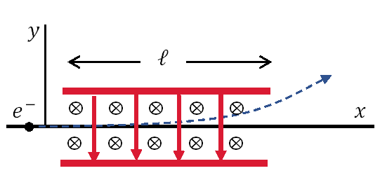
Fig. 3.2 Thomson’s method of measuring the electron charge to mass ratio was to send electrons through a region containing a magnetic field (\(\vec{B}\) into page) perpendicular to an electric field (\(\vec{E}\) down).

The ratio \(q/m\) can be determined if the initial velocity \(v_o\) is known. The initial velocity can be determined by turning on the magnetic field and adjusting the strength of \(\vec{B}\) until no deflection occurs. The condition for zero deflection is the case of equilibrium or

(3.3)\[\begin{align} \vec{F} = q\vec{E} + q\vec{v} \times \vec{B} = 0, \end{align}\]

and

\[ \vec{E} = -\vec{v} \times \vec{B}.\]

Since \(\vec{v}\) and \(\vec{B}\) are perpendicular (i.e., the cross-product \(\sin \theta = 1\)), the initial velocity is related to the electric and magnetic field strengths by

(3.4)\[v_x = v_o = E/B.\]

We can extract the ratio \(q/m\) through substitution by

(3.5)\[\begin{align} \frac{q}{m} = \frac{v_o^2 \tan \theta}{E\ell} = \frac{E\tan \theta}{B^2 \ell}. \end{align}\]

Exercise 3.1

An undergraduate that is reproducing Thomson’s experiment uses deflecting plates that are \(5.0\ {\rm cm}\) in length with an electric field of \(1.2 \times 10^4\ {\rm V/m}\). Without the magnetic field, we find an angular deflection of \(30^\circ\) and no deflection with a magnetic of \(8.8 \times 10^{-4}\ {\rm T}\). What is the initial velocity of the electron and its \(q/m\)?

For the case of no deflection, we only need to know the magnitudes of the electric \(E\) and magnetic \(B\) fields. Since those are given, we can solve for the initial velocity directly as

\[ v_o = \frac{E}{B} = \frac{1.2 \times 10^4\ {\rm V/m}}{8.8 \times 10^{-4}\ {\rm T}} = 1.4 \times 10^7\ {\rm m/s}. \]

The unit of one Tesla \({\rm T}\) represents a \(\frac{{\rm N\ s}}{{\rm C\ m}}\) and one Volt \({\rm V}\) represents a \(\frac{{\rm N\ m}}{{\rm C}}\). Therefore the units of \({\rm C}\) and \({\rm N}\) cancel, leaving only \({\rm m/s}\).

Using the given angular deflection and plate length, the charge to mass ratio is

\[ \frac{q}{m} = \frac{E\tan \theta}{B^2 \ell} = \frac{(1.2 \times 10^4\ {\rm V/m})(\tan 30^\circ)}{(8.8 \times 10^{-4}\ {\rm T})^2(0.05\ {\rm m})} = 1.8 \times 10^{11}\ {\rm C/kg}.\]

import numpy as np

E_mag = 1.2e4 #Electric field strength in V/m
B_mag = 8.8e-4 #Magnetic field strength in T

l_plate = 0.05 #plate length in m
deflect_ang = np.radians(30) #deflection angle in radians

v_o = E_mag/B_mag
q_m = E_mag*np.tan(deflect_ang)/(B_mag**2*l_plate)

print("The initial velocity of the electron is %1.1e m/s.\n" % v_o)
print("The charge to mass ratio is %1.1e C/kg." % q_m)

The initial velocity of the electron is 1.4e+07 m/s.

The charge to mass ratio is 1.8e+11 C/kg.

Thomson’s actual experiment obtained a result about 35% lower than the presently accepted value \(e/m = 1.76 \times 10^{11}\ {\rm C/kg}\). Thomson realized that the value of \(e/m\) for an electron was much larger than anticipated and a factor of \(10^3\) larger than the \(q/m\) previously measured for the hydrogen atom. He concluded that \(m\) was small, \(e\) was large, or both. In addition, the “carriers of the electricity” were quite penetrating compared with atoms or molecules, which must be larger in size.

3.2. Determination of Electron Charge

After Thomson’s measurement of \(e/m\), several investigators attempted to determine the actual magnitude of the electron’s charge. Robert Millikan in 1911 reported evidence for an accurate determination of the electron’s charge. Millikan’s classic experiment visually measured the motion of charged (positively and negatively) and uncharged oil drops under the influence of electrical and gravitational forces.

Fig. 3.3 Simplified scheme of Millikan’s oil-drop experiment. Image Credit: Wikipedia.

When an oil drop falls downward through the air, it experiences a frictional force \(\vec{F}_j\) that is proportional to its velocity due to the air’s viscosity by

(3.6)\[\vec{F}_j = -b\vec{v}.\]

This drag force always opposes the velocity, hence the negative sign. The constant \(b\) is determined via Stokes’ law and is proportional to the oil drop’s radius. Millikan showed that Stokes’ law was incorrect for small-diameter spheres due to the atomic nature of the medium, where an appropriate correction was required. For a first-order calculation, we neglect the buoyancy of the air that produces an upward force on the drop.

To suspend the oil drop at rest between the plates, the electric and gravitational forces must be balanced. This makes the frictional force equal to zero because the oil drop’s velocity is zero. The force balance is

(3.7)\[\begin{align} \vec{F}_E = q\vec{E}=-m\vec{g}, \quad (\text{when } v=0). \end{align}\]

The magnitude of the electric field is \(E=V/d\), which depends on the voltage \(V\) across large, flat plates separated by a small distance \(d\). The magnitude of the electron charge is determined as

(3.8)\[q = \frac{mgd}{V}.\]

To calculate \(q\), we need to know the mass \(m\) of the oil drops. Millikan found he could determine \(m\) by measuring the terminal velocity of the oil drop while the electric field was off. From Stoke’s law (or Eqn. (3.6)), the radius of the oil drop is related to the terminal velocity. Using the radius \(r\) and the density \(\rho\) of the oil, the mass of the oil can be determined by

(3.9)\[\begin{align} m = \frac{4}{3}\pi r^3 \rho. \end{align}\]

The oil drop can be moved up and down in the apparatus at will by adjusting the voltage magnitude and polarity. millikan reported that he was able to observe an oil drop for up to six hours, where the drop changed its charge several times. Millikan made 1000s of measurements using different oils and showed that there is a basic quantized electron charge. Millikan’s value was very close to the modern value \(e=1.602 \times 10^{-19}\ {\rm C}\).

Note

We always quote a positive number for the charge \(e\) and the charge on an electron is then \(-e\).

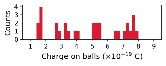
In an actual undergraduate laboratory experiment, students used plastic balls of about \(1\ \mu{\rm m}\) in diameter in place of the oil drops. This avoids the measurement of the oil drop’s terminal velocity and the dependence on Stokes’ law. the small plastic balls are sprayed through an atomizer in a liquid solution, which quickly evaporates. The balls are observed through a microscope. To make it easier for the charge on a ball to change, the region between the plates is bombarded occasionally with beta particle (electron) radiation from a radioactive source.

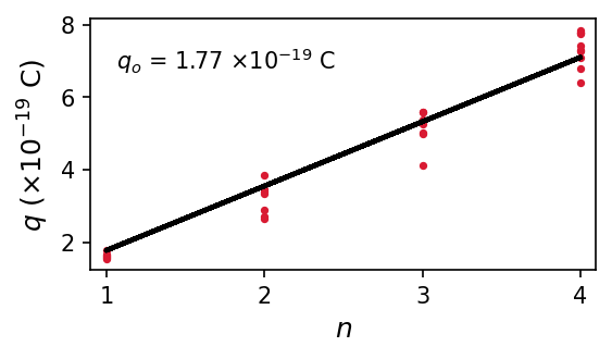
The table under the dropdown menu provides the first 30 (out of 100) measurements. The first python code produces a histogram with \(0.2 \times 10^{-19}\ {\rm C}\) sized bins. Due to the experimental setup, multiple charges can exist on the balls. We can account for this using the model \(q = n q_o\), where \(q_o\) represents the basic charge and \(n\) is an integer (starting from 1). The second python codes uses the data to find a best-fit value of \(q_o = 1.77 \times 10^{-19}\ {\rm C}\). The percentage error (using only the first 30 measurements) of this experiment is about \(10.7\%\). Using all the measurements, produces a best-fit value of \(q_o = 1.6 \times 10^{-19}\ {\rm C}\), which is much closer to the true value.

Click to reveal a table of observations!

Particle	Voltage (V)	\(\mathbf{q}\ (\times 10^{-19}\ {\rm C})\)	Particle	Voltage	q	Particle	Voltage	q
1	-30	-7.43	11	-126.3	-1.77	21	-31.5	-7.08
2	+28.8	+7.74	12	-83.9	-2.66	22	-66.8	-3.34
3	-28.4	-7.85	13	-44.6	-5.00	23	+41.5	+5.37
4	+30.6	+7.29	14	-65.5	-3.40	24	-34.8	-6.41
5	-136.2	-1.64	15	-139.1	-1.60	25	-44.3	-5.03
6	-134.3	-1.66	16	-64.5	-3.46	26	-143.6	-1.55
7	+82.2	+2.71	17	-28.7	-7.77	27	+77.2	+2.89
8	+28.7	+7.77	18	-30.7	-7.26	28	-39.9	-5.59
9	-39.9	-5.59	19	+32.8	+6.8	29	-57.9	-3.85
10	+54.3	+4.11	20	-140.8	+1.58	30	+42.3	+5.27

import numpy as np
import matplotlib.pyplot as plt

fs = 'large'
col = (218/256., 26/256., 50/256.)

data = np.genfromtxt("https://raw.githubusercontent.com/saturnaxis/ModernPhysics/main/Chapter_3/oil_drop.csv",delimiter=',')

fig = plt.figure(figsize=(4,1),dpi=150)
ax = fig.add_subplot(111)

ax.hist(np.abs(data[:,2]),bins=np.arange(0,10,0.2),color=col)
ax.set_xticks(np.arange(1,10))
ax.set_yticks(np.arange(0,5))
ax.set_xlim(0.5,9.5)

ax.set_ylabel("Counts",fontsize=fs)
ax.set_xlabel("Charge on balls ($\\times 10^{-19}\ {\\rm C})$",fontsize=fs);

import numpy as np
import matplotlib.pyplot as plt
from scipy.optimize import curve_fit
from scipy.constants import e

fs = 'large'
col = (218/256., 26/256., 50/256.)

def model(n,q0):
    return n*q0

data = np.genfromtxt("https://raw.githubusercontent.com/saturnaxis/ModernPhysics/main/Chapter_3/oil_drop.csv",delimiter=',')
q = np.abs(data[:,2])

fig = plt.figure(figsize=(4,2),dpi=150)
ax = fig.add_subplot(111)

#fit to model q = n*q_o; n= 1,2,3,...
n = q // 2 + 1

popt, pcov = curve_fit(model, n, q)
pct_error = np.abs(popt[0]*1e-19-e)/e*100
print("The error is %1.1f percent." % pct_error)

ax.plot(n,q,'.',ms=5,color=col)
ax.plot(n,model(n,*popt),'k-',lw=2)

ax.text(0.05,0.8,'$q_o$ = %1.2f $\\times 10^{-19}\ {\\rm C}$' % popt[0],transform=ax.transAxes)
ax.set_xticks(np.arange(1,5))
ax.set_xlim(0.9,4.1)

ax.set_xlabel("$n$",fontsize=fs)
ax.set_ylabel("$q$ ($\\times 10^{-19}\ {\\rm C})$",fontsize=fs);

The error is 10.7 percent.

3.3. Line Spectra

Thermal bodies produce a smooth, continuous radiation spectrum (intensity vs. wavelength), where chemical elements produce unique wavelengths (or colors) when burned in a flame or excited in an electrical discharge. Scientists used prisms (at least since Newton) to break light apart into their constituent colors for examination. Henry Rowland made high quality diffraction gratings, which made optical spectroscopy an important area of experimental physics.

Note

Rowland was one of the first six professors chosen in 1875 for the founding of Johns Hopkins University and was one of the foremost American physicists during that time, together with Michelson. Rowland was the first president of the American Physical Society in 1899, where Michelson was the vice president. Neither Rowland nor Michelson had formally earned a Ph.D. degree.

Fig. 3.4 Schematic of a grating spectrometer. Image Credit: Wikipedia.

A spectrometer (see Fig. 3.4) uses the light produced by a low-pressure gas contained in a tube, when an electrical discharge excites the atoms in the gas. The collimated light passes through a diffraction grating (with many ruling lines per centimeter) and the diffracted light is separated at an angle \(\theta\) depending on its wavelength \(\lambda\). The diffraction maxima are described mathematically by

(3.10)\[d \sin \theta = n\lambda,\]

which depends on the distance between rulings \(d\) and the order number \(n\) (an integer). Figure 3.5 illustrates the resulting pattern of light bands and dark areas (on the right) from a hydrogen gas tube (on the left). The pattern is called a line spectrum.

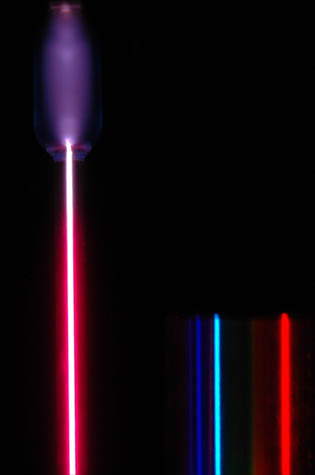
Fig. 3.5 At left is a hydrogen spectral tube excited by a 5000 volt transformer. The three prominent hydrogen lines are shown at the right of the image through a 600 lines/mm diffraction grating. Figure Credit: Hyperphysics.

Robert Bunsen and Gustav Kirchhoff realized that the wavelength of these line spectra constituted a fingerprint for the chemical elements and the identification for the composition of materials. The field of spectroscopy flourished due to the continual improvements made to diffraction gratings (i.e., finer and more evenly ruled gratings). Particular attention was paid to the Sun’s spectrum in hopes of understanding the origin of sunlight. The element helium was actually “discovered” by its line spectra from the Sun before it was recognized on Earth.

Scientists of the 1800s attempted to find some simple underlying order for the characteristic wavelengths of line spectra (i.e., why are the lines different for each element?). Hydrogen appeared to have the simplest looking spectrum and some chemists thought hydrogen atoms might build up to make more complex atoms. Johann Balmer in 1885 succeeded in obtaining a simple empirical formula that fit the wavelengths of the (then known) four lines in the hydrogen spectrum and several ultraviolet (UV) lines that were found in the spectra of white stars.

Note

When a formula is derived empirically, it is typically based on measurements of a few fundamental parameters. The coefficient(s) of the formula denote an approximation of some other unknown (perhaps fundamental) quantities. This is not to be confused with analytical formula, which is derived from first principles and expressed solely in terms of well-known fundamental quantities.

The Balmer series is described by

(3.11)\[\lambda = 364.56 \left( \frac{k^2}{k^2-4}\right)\ {\rm nm},\]

where the integer \(k\) (starting from 3) produces wavelengths that match all the visible hydrogen lines.

Note

Wavelengths were formerly listed in units of angstroms (Å) which are named after Anders Ångstrom. Ångstrom was one of the first people to observe and measure the wavelengths of the four visible lines of hydrogen. \(1\ {\rm \unicode{x212B}} = 0.1\ {\rm nm} = 10^{-10}\ {\rm m}\).

Equation (3.11) can be rewritten as its reciprocal into the following form

(3.12)\[\begin{align} \frac{1}{\lambda} = \frac{1}{365.56\ {\rm nm}}\left(\frac{k^2 -4}{k^2}\right) = \frac{4}{365.56\ {\rm nm}}\left( \frac{1}{2^2}-\frac{1}{k^2}\right) = R_{\rm H} \left( \frac{1}{2^2}-\frac{1}{k^2}\right), \end{align}\]

where \(R_{\rm H}\) represents the Rydberg constant (for hydrogen) and \(k\) is an integer. The ratio (\(4/364.56\ {\rm nm}\)) is \(1.0972 \times 10^7\ {\rm m^{-1}}\), where the more accurate value is \(1.096776 \times 10^7\ {\rm m^{-1}}\). Johannes Rydberg and Walther Ritz determined a more general empirical equation for calculating the wavelengths known as the Rydberg equation, given by

(3.13)\[\frac{1}{\lambda} = R_{\rm H}\left(\frac{1}{n^2}-\frac{1}{k^2}\right),\]

and is generalized as long as \(k>n\). The Balmer series is a special case of the Rydberg equation, when \(n=2\). By 1925, the five series related to the hydrogen atom’s spectral lines were discovered, where each series corresponded to a different integer \(n\). The understanding of the Rydberg equation and the discrete spectrum of hydrogen helped uncover the mysteries of the atom in the early 20th century.

Discoverer (year)	Wavelength	\(n\)	\(k\)
Lyman (1916)	Ultraviolet (UV)	1	\(>1\)
Balmer (1885); translated from German	Visible, Ultraviolet (UV)	2	\(>2\)
Paschen (1908); in German	Infrared (IR)	3	\(>3\)
Brackett (1922)	Infrared (IR)	4	\(>4\)
Pfund (1924)	Infrared (IR)	5	\(>5\)

Exercise 3.2

The visible lines of the Balmer series were observed first because they are the most easily seen (i.e., visible!). Show that the wavelengths of spectral lines in the Lyman (\(n=1\)) and Paschen (\(n=3\)) are not in the visible region (\(\lambda = 400-700\ {\rm nm}\)). Find the wavelengths of the four visible atomic hydrogen lines.

For a given \(n\) in the Rydberg equation (Eqn. (3.13)), the wavelength decreases with \(k\) because \(R_{\rm H}^{-1} \approx 91.174\ {\rm nm}\) and the difference in parentheses of the Rydberg equation can only cause this value to decrease after the first permissible \(k\). For comparing wavelengths in a series, it is sometimes more useful to represent the Rydberg equation as

\[ \lambda = R_{\rm H}^{-1}\left(\frac{n^2k^2}{k^2-n^2}\right), \]

for a finite \(k\).

Using the above expression, we can examine the wavelengths of each series (Lyman, Balmer, and Paschen) for hydrogen in turn.

For the Lyman series: \(n=1\)

\[\begin{align*} k=2:& \quad \lambda = 91.174\left(\frac{1^22^2}{2^2-1^2}\right) = 121.57\ {\rm nm}\ \text{(UV)} \\ k=3:& \quad \lambda = 91.174\left(\frac{1^23^2}{3^2-1^2}\right) = 102.57\ {\rm nm}\ \text{(UV)} \\ \end{align*}\]

All the wavelengths in the Lyman series are in the UV region and not visible by eye.

For the Balmer series: \(n=2\)

\[\begin{align*} k=3:& \quad \lambda = 91.174\left(\frac{2^23^2}{3^2-2^2}\right) = 656.47\ {\rm nm}\ \text{(Red)} \\ k=4:& \quad \lambda = 91.174\left(\frac{2^24^2}{4^2-2^2}\right) = 486.27\ {\rm nm}\ \text{(Blue-green)} \\ k=5:& \quad \lambda = 91.174\left(\frac{2^25^2}{5^2-2^2}\right) = 434.17\ {\rm nm}\ \text{(Violet)} \\ k=6:& \quad \lambda = 91.174\left(\frac{2^26^2}{6^2-2^2}\right) = 410.29\ {\rm nm}\ \text{(Violet)} \\ k=7:& \quad \lambda = 91.174\left(\frac{2^27^2}{7^2-2^2}\right) = 397.12\ {\rm nm}\ \text{(UV)} \\ \end{align*}\]

The first four wavelengths in the Balmer series are in the visible, although the \(k=6\) line is difficult to see due to its weak intensity.

For the Paschen series: \(n=3\)

\[\begin{align*} k=4:& \quad \lambda = 91.174\left(\frac{3^24^2}{4^2-3^2}\right) = 1875.63\ {\rm nm}\ \text{(IR)} \\ k=5:& \quad \lambda = 91.174\left(\frac{3^25^2}{4^2-5^2}\right) = 1282.17\ {\rm nm}\ \text{(IR)} \\ k=\infty:& \quad \lambda = 91.174\left(\frac{1}{3^2} - \frac{1}{\infty}\right)^{-1} = 820.59\ {\rm nm}\ \text{(IR)} \\ \end{align*}\]

All the wavelengths in the Paschen series are in the IR region and are not visible by eye. The higher series \(n\geq 4\), will all have wavelengths well above the visible region.

import numpy as np

def Rydberg_wavelength(n,k):
    #Calculates the wavelength using the Rydberg equation
    # n = integer; denotes type of series
    # k = integer; denotes the kth line of a series
    if np.isfinite(k):
        return (1./Rydberg)*(n**2*k**2)/(k**2-n**2)/1.e-9
    else:
        return (1./Rydberg)*1./(1./n**2-1./k**2)/1e-9
Rydberg = 1.096776e7 #Rydberg constant in m^-1
series = [1,2,3]
series_names = ["Lyman","Balmer","Paschen"]
k_vals = [[2,3],[3,4,5,6,7],[4,5,np.inf]]

for s in series:
    for k_v in k_vals[s-1]:
        H_lambda = np.round(Rydberg_wavelength(s,k_v),2)
        if np.isfinite(k_v):
            print("%s: (%i,%i) --> %3.2f nm." % (series_names[s-1],s,k_v,H_lambda))
        else:
            print("%s: (%i,infty) --> %3.2f nm." % (series_names[s-1],s,H_lambda))

Lyman: (1,2) --> 121.57 nm.
Lyman: (1,3) --> 102.57 nm.
Balmer: (2,3) --> 656.47 nm.
Balmer: (2,4) --> 486.27 nm.
Balmer: (2,5) --> 434.17 nm.
Balmer: (2,6) --> 410.29 nm.
Balmer: (2,7) --> 397.12 nm.
Paschen: (3,4) --> 1875.63 nm.
Paschen: (3,5) --> 1282.17 nm.
Paschen: (3,infty) --> 820.59 nm.

3.4. Quantization

Some Greek philosophers believed that matter must be composed of fundamental units, where the atom means “not further divisible.” Today think that some elements of matter are indivisible, which are the elementary particles that make up the atom. If there are building blocks of matter, then there must be some basic units of mass-energy of which matter is composed.

Building up matter from smaller parts implies that the smaller parts are quantized, or well-defined packets of mass-energy. Millikan’s oil drop experiment showed the quantization of electric charge \(q_o = e\). Modern theories predict that charges are quantized in units (called quarks) of \(\pm e/3\) and \(\pm 2e/3\). The charges of particles that have been directly observed are quantized in units of \(\pm e\).

The measured atomic weights are not continuous, where they have only discrete values. Molecules are formed from an integral (whole number) of atoms. For example, water is composed of exactly two hydrogen atoms and one oxygen atom. An organ pipe produces one fundamental musical note with overtones is a form of quantization arising from fitting a precise number (or fractions) of sound waves into the pipe (see Fig. 3.6). Line spectra are another examples of quantization, where the precise wavelengths can be described empirically by simple equations.

Fig. 3.6 The fundamental and three lowest overtones for a tube closed at one end. All have maximum air displacements at the open end and none at the closed end. Figure Credit: OpenStax: University Physics Vol 1.

3.5. Blackbody Radiation

When matter is heated, it emits radiation. This is nothing new if you’ve been around a campfire or forge. We can feel heat radiation emitted by the heat element on a electric stove, and the color of the element changes from dark red \((550^\circ{\rm C})\) to bright red \((700^\circ{\rm C})\). If the temperature were increased further, the color would progress through orange, yellow, and finally white. Physicists of the 19th century measured the intensity of the emitted radiation as a function of material, temperature, and wavelength.

All bodies emit and absorb radiation. The body is in thermal equilibrium with its surroundings when a its temperature is constant in time. For this to occur, the rate of emitted radiation must equal the rate absorbed. This implies a good thermal emitter is also a good absorber. The simplest (or most idealized) case is called a blackbody, which absorbs all the radiation falling onto it and reflects none. The simplest way to construct a blackbody is to drill a small hole in a hollow container (or cavity), where radiation enters and is eventually absorbed after many reflections (see Fig. 3.7). Only a small fraction of the entering rays will exit through the hole. If the blackbody is in thermal equilibrium, then it must also be an excellent emitter of radiation.

Fig. 3.7 An approximate realization of a black body as a tiny hole in an insulated enclosure. Image Credit: Wikipedia.

The radiation properties of the blackbody are independent of the composition of the container. Physicists study the properties of intensity vs. wavelength (i.e., spectral distribution) at fixed temperatures without having to know the details of emission or absorption by a particular kind of atom.

The intensity \(\mathcal{I}(\lambda,T)\) is the total power radiated per unit area per unit wavelength at a given temperature. Two important points about a spectrum are:

1. The maximum of the distribution shifts to smaller wavelengths as the temperature is increased.

2. The total power radiated increases with the temperature.

The first point is described mathematically as Wien’s displacement law:

(3.14)\[\lambda_{\rm max}T = 2.898 \times 10^{-3}\ {\rm m \cdot K} = 2.898 \times 10^6\ {\rm nm \cdot K},\]

where the wavelength \(\lambda_{\rm max}\) is found at the peak of the spectral distribution for a given temperature. We can see in Fig. 3.8 that the position of \(\lambda_{\rm max}\) varies with temperature as prescribed by Wien’s displacement law.

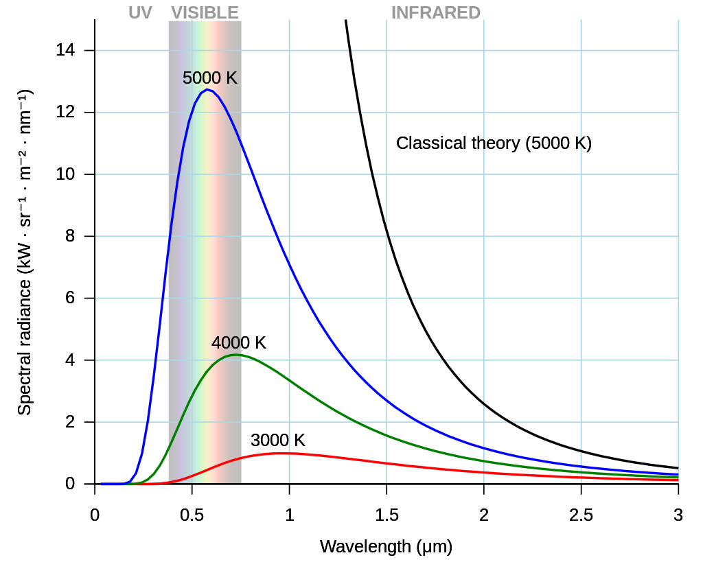
Fig. 3.8 As the temperature of a blackbody decreases, its intensity also decreases and its peak moves to longer wavelengths. Image Credit: Wikipedia.

Wilhelm Wien received the Nobel Prize in 1911 for his discoveries concerning radiation. We can quantify the second point (concerning the total power) by integrating the function \(\mathcal{I}(\lambda, T)\) over all wavelengths to find the power per unit area at temperature \(T\) as

\[ R(T) \int_0^\infty \mathcal{I}(\lambda, T) d\lambda. \]

Josef Stefan determined a empirical formula for \(R(T)\) in 1879, while Boltzmann derived it theoretically a few years later. They showed that \(R(T)\) is related to the temperature \(T\) by

(3.15)\[\begin{split}R(T) &= \epsilon \sigma T^4,\\\end{split}\]

which depends on the experimentally determined constant \(\sigma = 5.6705 \times 10^{-8}\ {\rm W/\left(m^2\cdot K^4\right)}\) called the Stefan-Boltzmann constant and is part of the Stefan-Boltzmann law \(R(T)\). This formula can be applied to any material with a known emissivity \(\epsilon\). The emissivity is simply the ratio of the emissive power of an object to that of an ideal blackbody. For an ideal blackbody, \(\epsilon = 1\) and therefore, the value for emissivity is always less than 1. Equation (3.15) is valid for experiments on Earth and for measuring the properties of stars.

Exercise 3.3

A furnace has walls that reach \(1600^\circ{\rm C}\), when it is in use. What is the wavelength of maximum intensity emitted when a small door is opened?

The wavelength of maximum intensity is just \(\lambda_{\rm max}\), which means we can apply Wien’s displacement law. First, we convert the temperature to Kelvin

\[ T = (1600 + 273.15)\ {\rm K} = 1873.15\ {\rm K}.\]

Then, Wien’s law is applied to find the peak wavelength

\[ \lambda_{\rm max} = \frac{2.898 \times 10^6\ {\rm nm \cdot K}}{1873.15\ {\rm K}} = 1547\ {\rm nm}. \]

The peak wavelength lies in the infrared (IR) region of the EM spectrum.

from scipy.constants import Wien, zero_Celsius
import numpy as np

T_wall = 1600 #temperature of the furnace wall in ^oC
T_K = T_wall + zero_Celsius # convert temperature into K

def lambda_max(T):
    #find the peak wavelength of a material given a temperature
    return Wien/T/1e-9 #returns the peak wavelength (in nm)

print("The peak wavelength is %i nm." % np.round(lambda_max(T_K),0))

The peak wavelength is 1547 nm.

Exercise 3.4

The peak wavelength of the Sun’s spectral distribution is measured to be near \(500\ {\rm nm}\). Assuming that the Sun is a blackbody, calculate (a) the Sun’s effective surface temperature, (b) the total power per unit area \(R(T)\) emitted from the Sun’s surface, and (c) the energy received by the Earth each day.

(a) Since we assume that the Sun behaves like an ideal blackbody (\(\epsilon=1\)), then we can use Wien’s displacement law to determine its temperature \(T\) at the surface by

\[ T_{\rm surf} = \frac{2.898 \times 10^6\ {\rm nm\cdot K}}{500\ {\rm nm}} = 5800\ {\rm K}.\]

(b) The total power per unit area at \(5800\ {\rm K}\) is calculated by the Stefan-Boltzmann law as

\[\begin{align*} R(T) &= \epsilon \sigma T^4 = \sigma T^4 \\ & = \left(5.6705 \times 10^{-8}\ {\rm W/\left(m^2\cdot K^4\right)}\right)(5800\ {\rm K})^4 = 6.40 \times 10^7\ {\rm W/m^2}. \end{align*}\]

(c) The amount of power the Earth receives is determined by the total power from the Sun, which modifies the Stefan-Boltzmann law to include the surface area of the Sun as

\[\begin{align*} P_{\rm Sun} &= (4\pi r_{Sun}^2)R(T) \\ &= (6.082 \times 10^{18}\ {\rm m^2})(6.40 \times 10^7\ {\rm W/m^2}) = 3.89 \times 10^{26}\ {\rm W}. \end{align*}\]

Then, we need to determine the radiative flux \(F\) received at 1 astronomical unit (AU) from the Sun, where \(1\ {\rm AU} = 1.495 \times 10^{11}\ {\rm m}\). The radiative flux is given as

\[ F = \frac{P_{Sun}}{4\pi d^2} = \frac{3.89 \times 10^{26}\ {\rm W}}{4\pi\left(1.495 \times 10^{11}\ {\rm m}\right)^2} = 1380\ {\rm W/m^2}. \]

Measurements of the Sun’s radiation outside the Earth’s atmosphere vary slightly throughout year given the small changes in \(d\), where the average value is called the Solar Constant and is equal to \(1360\ {\rm W/m^2}\). Our calculation is a little high because the Sun’s actual surface temperature is a little lower \((T_\odot = 5777\ {\rm K})\) than our estimate using the Stefan-Boltzmann law. However, it does show that the Sun does act as a blackbody.

from scipy.constants import Wien, sigma, astronomical_unit
import numpy as np

def T_surf(l_max):
    #determine the surface temperature given the peak wavelength l_max (in nm)
    return (Wien*1e9)/l_max #return the surface temperature in K
def Stef_Boltz(T):
    #calculate the total power (in W/m^2) for a given temperature T
    return sigma*T**4
def surf_area(R):
    #calculate the surface area of a sphere of radius R (in m)
    return 4*np.pi*R**2
def flux(Rad,R,d):
    #calculate the flux received at a distance d
    #Rad = total power per unit area (in W/m^2)
    #R = radius of the Sun (in m)
    #d = distance to the Sun (in m)
    return (Rad*surf_area(R))/(4.*np.pi*d**2)

lmax_sun = 500 #peak wavelength (in nm) observed for the Sun
T_sun = T_surf(lmax_sun)
Rad_Sun = Stef_Boltz(T_sun)

R_sun = 6.95700e8 #radius of the Sun (in m) as defined by the IAU; https://en.wikipedia.org/wiki/Solar_radius
R_earth = 6.3781e6 #radius of the Earth (in m); https://en.wikipedia.org/wiki/Earth_radius 

flux_AU = flux(Rad_Sun,R_sun,astronomical_unit)

print("The Sun's surface temperature is %i K.\n" % np.round(T_sun,-1))
print("The total power emitted by the Sun per unit area is %1.2e W/m^2.\n" % Rad_Sun)
print("The total power received by the Earth per unit area is %i W/m^2." % np.round(flux_AU,-1))

The Sun's surface temperature is 5800 K.

The total power emitted by the Sun per unit area is 6.40e+07 W/m^2.

The total power received by the Earth per unit area is 1380 W/m^2.

Attempts to understand and derive (from basic principles) the shape of the blackbody spectral distribution (Fig. 3.8) were unsuccessful and presented a serious problem for scientists near the beginning of the 20th century. A blackbody’s radiation can be expressed as a superposition of electromagnetic waves (over a range of frequencies) within a cavity (i.e., a standing wave dependent on frequency). The equipartion theorem from thermodynamics assigns equal average energy \(kT\) to each possible wave configuration. But which wave configuration was the most probable?

In 1900, Lord Rayleigh showed that the blackbody spectral distribution should have a \(\lambda^{-4}\) dependence, where his derivation was based from classical theories of electromagnetism and thermodynamics. Later, Sir James Jeans helped Rayleigh determine the proportionality factor of the distribution, where their complete result (known as the Rayleigh-Jeans formula) is

(3.16)\[\mathcal{I}(\lambda, T) = \frac{2\pi ckT}{\lambda^4}.\]

It was the best formulation that classical theory could muster to describe blackbody radiation. For long wavelengths \((>10^4\ {\rm nm})\), the Rayleigh-Jeans formula provided a reasonable match to observations because there there are a few configurations by which a standing wave can form inside the cavity (see the hyperphysics page for more detail). However, as the wavelengths become shorter the number of standing wave possibilities increases. in the limit \(\lambda \rightarrow 0\), the total energy of all configurations becomes infinite because each standing wave has nonzero energy \(kT\).

Fig. 3.9 Comparison of the classical Rayleigh-Jeans Law and the Planck radiation formula (which matches the experimental data). Image Credit: Hyperphysics.

Figure 3.9 shows the result from the Rayleigh-Jeans formula compared to the Planck Radiation formula that better matches the experimental data. Note that it deviates badly at short wavelengths, where Paul Ehrenfest dubbed this situation as the “ultraviolet catastrophe” and was a phenomenon that classical physics could not explain.

Max Planck was an expert on the second law of thermodynamics, rejected Boltzmann’s statistical version of thermodynamics, and even doubted the atomic theory of matter. In 1889, Planck’s view began to change when he investigated the irreversibility of radiation processes. He that the laws of electromagnetism distinguished between past and present, but Boltzmann showed that there could be no difference. Planck then examined the problem of blackbody radiation.

Planck tried many functions to fit the measurements of \(\mathcal{I}(\lambda, T)\) and it wasn’t clear that he was even aware of Lord Rayleigh’s result. Planck reported is formula in 1900, but could not explain it fully. Plank assumed that the radiation in the cavity was emitted (and absorbed) by some sort of “oscillators” that were contain in the walls. Building on Hertz’s and Boltzmann’s work, he added up the energies of the oscillators and each oscillator had an energy that was an integral multiple of \(hf\) (\(h\) is a constant and \(f\) is the frequency of the oscillator). This was a technique invented by Boltzmann, where Planck expected tot ake the limit \(h\rightarrow 0\) to include all the possibilities. He noticed by keeping \(h>0\) that he arrived at the needed equation as

(3.17)\[\mathcal{I}(\lambda, T) = \frac{2\pi hc^2}{\lambda^5\left(e^{hc/(\lambda kT}) - 1\right)}.\]

Equation (3.17) is known as Planck’s radiation law. No matter what Planck tried, he could only find agreement with the experimental data if he made two modifications to the classical theory:

1. The oscillators (of electromagnetic origin) can only have discrete energies determined by \(E_n = nhf\), which depends on an integer \(n\), the oscillator frequency \(f\), and Planck’s constant \(h = 6.6261 \times 10^{-34}\ {\rm J\cdot s}\).

2. The oscillators can absorb or emit energy in the discrete multiples of the fundamental quantum of energy given by \(\Delta E = hf\).

Planck found these results quite disturbing and spent several years trying his initial plan so that \(h\rightarrow 0\). Each attempt failed and Planck’s quantum result become one of the cornerstones of modern physics.

Exercise 3.5

Show that Wien’s displacement law follows from Planck’s radiation law.

Wien’s law describes the maximum wavelength for the function \(\mathcal{I}(\lambda, T)\). Recall from calculus, that the maximum of a function is determined by the setting the first derivative equal to zero. Since it is the maximum wavelength, we take the first derivative with respect to \(\lambda\), or

\[\frac{ d\mathcal{I}(\lambda, T)}{d\lambda} = 0. \]

Using the product rule (or quotient rule), we have

\[\begin{align*} 2\pi hc^2\frac{d}{d\lambda}\left[\lambda^{-5}\left(e^{hc/(\lambda kT)} - 1\right)^{-1}\right] = 0, \\ 2\pi hc^2\left[-5\lambda^{-6}\left(e^{hc/(\lambda kT)} + 1\right)^{-1} - \frac{hc}{\lambda^7 kT}e^{hc/(\lambda kT)}\left(e^{hc/(\lambda kT)} - 1\right)^{-2}\right] = 0, \\ \frac{2\pi hc^2}{\lambda^6\left(e^{hc/(\lambda kT)} + 1\right)}\left[-5 - \frac{hc}{\lambda kT}e^{hc/(\lambda kT)}\left(e^{hc/(\lambda kT)} - 1\right)^{-1}\right] = 0, \\ \frac{\mathcal{I}(\lambda, T)}{\lambda}\left[-5 + \frac{hc}{\lambda kT}\frac{e^{hc/(\lambda kT)}}{\left(e^{hc/(\lambda kT)} - 1\right)}\right] = 0. \end{align*}\]

The trivial solution is that \(\mathcal{I}(\lambda, T) = 0\), which doesn’t fit the observations. Therefore the second term in brackets must be equal to zero, or

\[ -5 + \frac{hc}{\lambda kT}\frac{e^{hc/(\lambda kT)}}{\left(e^{hc/(\lambda kT)} - 1\right)} = 0.\]

Let’s try the transformation \(x = hc/(\lambda kT)\) and upon substitution, we get

\[ -5 + \frac{xe^x}{e^x-1} = 0, \]

and

\[ xe^x = 5(e^x-1).\]

This is a transcendental equation and can be solved numerically via a root finding method (e.g., bisection). The result is \(x\approx 4.965\) and

\[ \frac{hc}{\lambda_{\rm max}kT} = 4.965.\]

Wien’s displacement law is \(\lambda_{\rm max}T = \text{constant}\). Solving for the left hand side produces

\[\begin{align*} \lambda_{\rm max}T &= \frac{hc}{4.965k} \\ &= \frac{(6.6261 \times 10^{-34}\ {\rm J\cdot s})(3 \times 10^8\ {\rm m/s})}{4.965(1.38 \times 10^{-23}\ {\rm J/K})} \\ &= 2.898 \times 10^{-3}\ {\rm m\cdot K}, \end{align*}\]

which is the empirically determined Wien’s displacement law.

from scipy.optimize import bisect
from scipy.constants import h,c,k,Wien
import numpy as np

def x_trans(lam):
    #get x transformation given a value for lambda (wavelength in nm)
    return h*c/((lam*1e-9)*k*T)

def Wien_constant(x):
    #calculate the constant for Wien's law
    return h*c/(x*k)

def func(lam):
    #evaluate the transcendental equation 
    x = x_trans(lam)
    return x*np.exp(x) - 5*(np.exp(x) - 1.)
T = 6000 #trial temperature for hc/(lambda kT)
root = bisect(func, 100, 1000)
x_max = x_trans(root)
Wien_disp = Wien_constant(x_max)
pct_error = np.abs(Wien-Wien_disp)/Wien*100

print("The root of the transcendental equation is %1.3f.\n" % x_max)
print("The constant for Wien's displacement law is %1.3e m K.\n" % Wien_disp)
print("The error for Wien's displacement law constant is %1.2e percent." % pct_error)

The root of the transcendental equation is 4.965.

The constant for Wien's displacement law is 2.898e-03 m K.

The error for Wien's displacement law constant is 6.39e-09 percent.

3.6. Photoelectric Effect

The simplest evidence for the quantization of radiation energy comes from the explanation of the photoelectric effect. Hertz noticed that when UV light fell on a metal electrode, a charge was produced that separated the leaves of his electroscope. The photoelectric effect is on of the several ways electrons can be emitted by materials. By the early 20th century, it was known that electrons are bound to matter, where the “free” valence electrons are able to move easily from atom to atom and are not able to leave the surface. The methods now known by which electrons can escape the material include:

1. Thermionic emission: Application of heat allows electrons to gain enough energy to escape.

2. Secondary emission: The electron gains enough energy by transfer from a high-speed particle that strikes the material from outside.

3. Field emission: A strong external electric field pulls the electron out of the material.

4. Photoelectric effect: Incident light (EM radiation) shining on the material transfers energy to the electrons, which allows them to escape.

Electrons in metals are weakly bound, where light can give electrons enough extra kinetic energy to allow them to escape. The ejected electrons, or photoelectrons, are produce when the minimum extra kinetic energy equals the work function \(\phi\). The work function is the minimum binding energy of the electron to the material and thus, depends on the chemical makeup of the material.

Table 3.1 Work Functions: From Handbook of Chemistry and Physics

Element	\(\phi\ ({\rm eV})\)	Element	\(\phi\ ({\rm eV})\)	Element	\(\phi\ ({\rm eV})\)
Ag	4.64	K	2.29	Pd	5.22
Al	4.20	Li	2.93	Pt	5.64
C	5.0	Na	2.36	W	4.63
Cs	1.95	Nd	3.2	Zn	4.33
Cu	4.48	Ni	5.22	Zr	4.05
Fe	4.67	Pb	4.25

3.6.1. Experimental Results

Photoelectricity was studied using an experimental apparatus, where incident light falls on the emitter (i.e., the photocathode or cathode) that ejects electrons. Some of the electrons travel toward the collector (i.e., the anode), where either negative (retarding) or positive (accelerating) applied voltage \(V\) is imposed by the power supply. The current \(I\) measured in the ammeter (photocurrent) arises from the flow of photoelectons from emitter to collector. Figure 3.10 illustrates a schematic of the experimental setup.

Fig. 3.10 Schematic of the experiment to demonstrate the photoelectric effect. Filtered, monochromatic light of a certain wavelength strikes the emitting electrode (E) inside a vacuum tube. The collector electrode (C) is biased to a voltage \(V_C\) that can be set to attract the emitted electrons, when positive, or prevent any of them from reaching the collector when negative. Figure Credit: Wikipedia.

The experimental study of the photoelectric effect reveals that:

1. The kinetic energies of the photoelectrons are independent of the light intensity. A stopping potential (i.e., applied voltage) of \(-V_o\) is sufficient to stop all the photoelectrons, for any light intensity. For a given light intensity there is a maximum (saturation) photocurrent, which is reached as the applied voltage increases from negative to positive values.

2. The maximum kinetic energy of the photoelectrons depends on the frequency of the light and the composition of the emitting material. For light of different frequency a different retarding (slowing) potential \(-V_o\) is required to stop the most energetic photoelectrons. The value of \(V_o\) depends on the frequency \(f\) but not on the intensity.

3. The smaller the work function \(\phi\) of the emitter material, the lower is the threshold frequency of the light that can eject photoelectrons. No photoelectrons are produced for frequencies below this threshold frequency, for any light intensity.

4. When the photoelectrons are produced, their number is proportional to the light intensity. The maximum photocurrent is proportional to the light intensity.

5. The photoelectrons are emitted almost instantly (\(\leq 3\times 10^{-9}\ {\rm s}\)) following the illumination of the photocathode, which is independent of the light intensity.

Fig. 3.11 Diagram of the maximum kinetic energy as a function of the frequency of light on zinc. Photoelectrons are produced using \( f = 10.4 \times 10^{14}\ {\rm Hz}\) photons (i.e., UV (\(289\ {\rm nm}\)) photons). Image Credit: Wikipedia.

Except for result 5, these experimental observations were known in rudimentary form by 1902. This was primarily due to the work of Philipp Lenard, who extensively studied the photoelectric effect and received the Nobel Prize in Physics in 1905.

3.6.2. Classical Interpretation

Classical theory allows electromagnetic radiation to eject photoelectrons from matter, but the theory also predicts that the total amount of energy in a light wave increases as the light intensity increases. According to classical theory, the electrons should have more kinetic energy if the light intensity is increased.

• According to experimental result 1, a characteristic retarding potential \(-V_o\) is sufficient to stop all photoelectrons for a given light frequency \(f\). Classical EM theory is unable to explain this result.

• From result 2, the maximum kinetic energy of the photoelectrons depends on the value of the light frequency \(f\) and not on the light intensity. Classical theory cannot explain this result either.

• The existence of a threshold frequency is inexplicable in classical theory.

• Classical theory does predict the number of photoelectrons ejected will increase with intensity in agreement with experimental result 4.

• For extremely low light intensities, a long time would elapse before any one electron could obtain sufficient energy to escape. However, the photoelectrons are ejected almost immediately. Classical theory fails to explain result 5.

Exercise 3.6

Photoelectrons may be emitted from sodium \({\rm Na}\) (\(\phi = 2.36\ {\rm eV}\)) even for light intensities as low as \(10^{-8}\ {\rm W/m^2}\). Calculate classically how much time the light must shine to produce a photoelectron of kinetic energy of \(1\ {\rm eV}\).

We assume that all of the light is absorbed in the surface layer of atoms. We need to calculate the number of sodium atoms per unit area in the surface layer (i.e. 1 atom thick). We find the number of \({\rm Na}\) atoms/volume by (and looking up some key properties of \({\rm Na}\))

\[\begin{align*} \frac{\text{Avogadro's number}}{\text{Na gram molecular weight}} \times \text{density} &= \frac{\text{number of Na atoms}}{\text{volume}}, \\ \frac{6.02 \times 10^{23}\ {\rm atoms/mol}}{23\ {\rm g/mol}} \times 0.97 \frac{{\rm g}}{{\rm cm^3}} &= 2.54 \times 10^{22}\ \frac{\rm atoms}{\rm cm^3} = 2.54 \times 10^{28}\ \frac{\rm atoms}{\rm m^3}. \end{align*}\]

To estimate the thickness of one layer of atoms, we assume a cubic structure and

\[\begin{align*} \frac{1\ {\rm atom}}{d^3} &= 2.54 \times 10^{28}\ \frac{\rm atoms}{\rm m^3}, \\ d &= \left(\frac{1\ {\rm atom}}{2.54 \times 10^{28}\ \frac{\rm atoms}{\rm m^3} }\right)^{1/3} = 3.40 \times 10^{-10}\ {\rm m} = 0.34\ {\rm nm}. \end{align*}\]

If all the light is absorbed in the first layer of atoms, the number of exposed atoms per \({\rm m^2}\) is

\[ 2.54 \times 10^{28}\ \frac{\rm atoms}{\rm m^3} \times 3.40 \times 10^{-10}\ {\rm m} = 8.64 \times 10^{18}\ \frac{\rm atoms}{\rm m^2}. \]

With the intensity of \(10^{-8}\ {\rm W/m^2}\), each atom will receive energy at the rate of

\[\begin{align*} 10^{-8}\ {\rm W/m^2} \times \frac{1}{8.64 \times 10^{18}\ \frac{\rm atoms}{\rm m^2}} &= 1.16 \times 10^{-27}\ {\rm W}, \\ & = 7.25 \times 10^{-9}\ {\rm eV/s}. \end{align*}\]

To escape, the electrons need to attain an total energy of \(3.36\ {\rm eV}\ (= \phi + 1\ {\rm eV})\). Using the energy absorption rate for a single electron, we can find the time \(t\) needed to absorb the total energy by

\[ t = \frac{ 3.36\ {\rm eV}}{7.25\times 10^{-9}\ {\rm eV/s}} = 4.63 \times 10^8\ {\rm s} = 14.7\ {\rm years}. \]

Based on classical calculations, the time required to eject a photoelectron should be 15 years!

Tip

\[\begin{align*} 1\ {\rm W} &= 1\ \frac{\rm J}{\rm s} \times \frac{1}{1.6 \times 10^{-19}\ {\rm J/eV}} = 6.25 \times 10^{18}\ {\rm eV/s}\\ 1\ {\rm year} &= \frac{365.25\ {\rm days}}{1}\times \frac{24\ {\rm hr}}{1\ {\rm day}} \times \frac{3600\ {\rm s}}{1\ {\rm hr}} = 3.156 \times 10^7\ {\rm s} \end{align*}\]

from scipy.constants import eV, year, N_A

I_src = 1e-8 #Instensity of light in W/m^2
phi_Na = 2.36*eV #work function for Na (in J)
KE_pe = 1*eV #kinetic energy of a photoelectron
Tot_E = phi_Na + KE_pe
print("The total energy required to eject a 1 eV photoelectron from Na is %1.2e J or %1.2f eV.\n" % (Tot_E,Tot_E/eV))

Na_density = 0.968 #density of Na (in g/cm^3)
Na_molar_mass = 22.990 #molar mass of sodium in g/mol
Na_atoms_vol = N_A/Na_molar_mass*Na_density*1e6 #Na atoms/m^3
d_Na = 1./Na_atoms_vol**(1./3.) #thickness of one layer of Na atoms
Na_atom_area = Na_atoms_vol*d_Na #Na atoms/m^2

print("The number of atoms per unit volume in Na is %1.2e atom/m^3.\n" % Na_atoms_vol)
print("The thickness of one layer of Na atoms is %1.2e m or %1.2f nm.\n" % (d_Na,d_Na/1e-9))
print("The number of atoms of Na per unit area is %1.2e atom/m^2.\n" % Na_atom_area)

energy_rate = I_src/Na_atom_area #energy absorption rate of I_src
t_req = Tot_E/energy_rate/year #time required to eject a photoelectron in years

print("The energy rate for the Na atoms is %1.2e W. \n" % energy_rate)
print("The time required to eject a 1 eV photoelectron from Na is %2.1f years." % t_req)

The total energy required to eject a 1 eV photoelectron from Na is 5.38e-19 J or 3.36 eV.

The number of atoms per unit volume in Na is 2.54e+28 atom/m^3.

The thickness of one layer of Na atoms is 3.40e-10 m or 0.34 nm.

The number of atoms of Na per unit area is 8.63e+18 atom/m^2.

The energy rate for the Na atoms is 1.16e-27 W. 

The time required to eject a 1 eV photoelectron from Na is 14.7 years.

3.6.3. Einstein’s theory

Albert Einstein was intrigued by Planck’s hypothesis that the electromagnetic radiation field must be absorbed and emitted in quantized amounts. Einstein took Planck’s idea one step further and suggested that the electromagnetic radiation field itself is quantized. He also suggested in his 1905 paper (in German; in English) that

“the energy of a light ray spreading out from a point source is not continuously distributed over an increasing space but consists of a finite number of energy quanta which are localized at points in space, which move without dividing, and which can only be produced and absorbed as complete units.”

We now call the energy quanta of light: photons. According to Einstein, each photon has the energy quantum

(3.18)\[E = hf,\]

which only depends on the frequency \(f\) of the electromagnetic wave and Planck’s constant \(h\). The photon travels at the speed of light \(c\) in a vacuum, where its wavelength is given by

(3.19)\[\lambda f = c.\]

Einstein proposed that light should behave with its well-known wave-like aspect and light should also be considered to have a particle-like aspect. The quantum of light delivers it entire energy \(hf\) to a single electron in the material. To leave the material, the struck electron must give up an amount of energy \(\phi\) to overcome its binding in the material. The electron may lose some additional energy by electron interactions on its way to the surface. Whatever remaining energy will appear as the electron’s kinetic energy as it leaves the emitter. The conservation of energy requires that

(3.20)\[\begin{align} hf = \phi + \text{K.E. (electron)}. \end{align}\]

We are safe in using the nonrelativistic form of the electron’s kinetic energy \((\frac{1}{2}mv^2)\) because the energies involved are on the order of \({\rm eV}\). The electron’s energy will degrade as it passes through the emitter material. Experimentally, we detect the maximum value of the kinetic energy as

(3.21)\[\begin{align} hf = \phi + \frac{1}{2}mv^2_{\rm max}. \end{align}\]

The retarding potentials are opposing potentials needed to stop (i.e., work against) the most energetic electrons, or

(3.22)\[\begin{align} W = eV_o = \frac{1}{2}mv^2_{\rm max}. \end{align}\]

3.6.4. Quantum Interpretation

Classical Interpretation interpreted the experimental results using classical physics, but does the photoelectric effect (as explained by Einstein) explain all the data? The 1st and 2nd experimental results can be explained, where an electron’s kinetic energy does not depend on the light intensity at all. It depends only on the light frequency and the work function of the material through

(3.23)\[\frac{1}{2}mv^2_{\rm max} = eV_o = hf - \phi.\]

A potential that is slightly more positive than \(-V_o\) will not be able to repel all the electrons, and practically all the electrons will be collected when the retarding voltage is near zero. For very large positive potentials, all the electrons will be collected. If the light intensity increases, there will be more photons per unit area, more electrons ejected, and therefore, a higher photocurrent.

If a different light frequency is used, then a different stopping potential is required to stop the most energetic electrons. For a constant light intensity, a different stopping potential \(V_o\) is required for each \(f\), but the maximum photocurrent will not change because the number of photoelectrons ejected is constant. The quantum theory easily explains result 4.

Equation (3.23) predicts that the stopping potential will be linearly proportional to the light frequency, with a slope \(h/e\) and \(h\) is Planck’s constant. The slope is independent of the metal used to construct the photocathode, where Eqn. (3.23) can be rewritten as

(3.24)\[eV_o = \frac{1}{2}mv^2_{\rm max} = hf - hf_o = h\Delta f,\]

and the negative of the \(y\)-intercept is \(\phi = hf_o\). The frequency \(f_o\) represents the threshold frequency for the photoelectric effect. This explains experimental result 3.

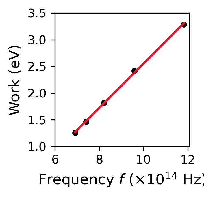
The data available in 1905 were not sufficiently accurate enough to prove (or disprove) Einstein’s theory, where Planck and others viewed the theory with skepticism. in 1916, Millikan confirmed Einstein’s prediction even though he set out to disprove it at the beginning of his investigation. Millikan found the value of \(h\) from the slope of a line for measurements of the kinetic energy and the photon frequency (see data in Table III). Millikan’s result is in good agreement with the modern value of \(h\) (see python code below). Due to the success of these explanations and predictions, Einstein received the Nobel Prize in 1922.

from scipy.constants import e,c,eV,h
import matplotlib.pyplot as plt
import numpy as np

#Values from Millikan (1916) Table III using deflections ~2-3 mm (assuming that +3.928 --> 0.928 as typo)
Na_lam = np.array([4339,4047,3650,3126,2535])*1e-10 #wavelengths in Angstroms converted to m
Na_Volts = np.array([-1.103,-0.9,-0.539,0.058,0.928]) #voltages

fs = 'large'
col = (218/256., 26/256., 50/256.)

fig = plt.figure(figsize=(2,2),dpi=300)
ax = fig.add_subplot(111)

x_coord, y_coord = c/Na_lam, e*Na_Volts/eV + 2.36 #shifted by \phi for Na
ax.plot(x_coord/1e14, y_coord,'k.',ms=8)
z = np.polyfit(x_coord, y_coord,1)
ax.plot(x_coord/1e14,np.poly1d(z)(x_coord),'-',lw=2,color=col)

print("The value of h from Millikan is %1.2e J s.\n" % (z[0]*eV))
pct_error = np.abs(z[0]*eV-h)/h*100
print("The error in Millikan's result is %2.1f percent." % pct_error)

ax.set_xticks(np.arange(6,14,2))
ax.set_yticks(np.arange(1,4,0.5))

ax.set_xlabel("Frequency $f$ ($\\times 10^{14}$ Hz)", fontsize=fs)
ax.set_ylabel("Work (eV)", fontsize=fs);

The value of h from Millikan is 6.65e-34 J s.

The error in Millikan's result is 0.4 percent.

The quantization of the electromagnetic radiation field tells us that electromagnetic radiation consists of photons, which are particle-like and each consists of energy

(3.25)\[E = hf = \frac{hc}{\lambda},\]

depending on the frequency \(f\) or wavelength \(\lambda\) of the photon. The total energy of a beam of light is the sum of the energy of all the photons, where a monochromatic (i.e., single color) light is an integral multiple of \(hf\). The photons have only one speed: the speed of light (\(=c\) in vacuum).

Exercise 3.7

A \(400\ {\rm nm}\) photon is incident upon lithium \((\phi = 2.93\ {\rm eV})\). Calculate (a) the photon energy and (b) the stopping potential \(V_o\).

(a) Since we know the wavelength of the photon, we can calculate is energy through

\[\begin{align*} E = \frac{hc}{\lambda} &= \frac{(6.626 \times 10^{-34}\ {\rm J\cdot s}),(3\times 10^8\ {\rm m/s})}{400 \times 10^{-9}}, \\ &= 4.97 \times 10^{-19}\ {\rm J}, \\ &= 3.10\ {\rm eV}. \end{align*}\]

(b) For the stopping potential, Eqn. (3.24) gives

\[\begin{align*} eV_o &= \frac{hc}{\lambda} - \phi = 3.10\ {\rm eV} - 2.93\ {\rm eV} = 0.17\ {\rm eV}, \\ V_o &= 0.17\ {\rm V}. \end{align*}\]

A retarding potential of \(0.17\ {\rm V}\) will stop all photoelectrons.

from scipy.constants import h,c,eV

phi_Li = 2.93 #work function for lithium in eV
E_400 = h*c/400e-9 #energy of a 400 nm photon in J
print("The energy of a 400 nm photon is %1.2e J or %1.2f eV.\n" % (E_400,E_400/eV))

V_o = E_400/eV - phi_Li
print("The stopping potential for a 400 nm photon on lithium is %1.2f V." % V_o)

The energy of a 400 nm photon is 4.97e-19 J or 3.10 eV.

The stopping potential for a 400 nm photon on lithium is 0.17 V.

Exercise 3.8

(a) What frequency of light is needed to produce electrons \(3\ {\rm eV}\) electrons from the illumination of lithium? (b) Find the wavelength of this light and where it lies in the electromagnetic spectrum.

(a) From the previous example, we know the work function for lithium \((\phi = 2.93\ {\rm eV})\). Through conservation of energy, the energy of the light is equal to the total energy of the electron, or

\[\begin{align*} hf &= \phi + \frac{1}{2}mv_{max}^2, \\ &= 2.93\ {\rm eV} + 3\ {\rm eV} = 5.93\ {\rm eV}, \\ &= 9.50 \times 10^{-19}\ {\rm J}. \end{align*}\]

The photon frequency is now found to be

\[ f = \frac{E}{h} = \frac{9.50 \times 10^{-19}\ {\rm J}}{6.6261 \times 10^{-34}\ {\rm J\cdot s}} = 1.43 \times 10^{15}\ {\rm Hz}. \]

(b) The wavelength of the light can be found from \(c = \lambda f\), which is

\[\begin{align*} \lambda &= \frac{c}{f}, \\ &= \frac{3\times 10^8\ {\rm m/s}}{1.43 \times 10^{15}\ {\rm Hz}}, \\ &= 2.09 \times 10^{-7}\ {\rm m}, \\ & = 209\ {\rm nm}. \end{align*}\]

This photon is in the UV \((\lambda <400\ {\rm nm})\) portion of the electromagnetic spectrum.

from scipy.constants import h, eV, c

phi_Li = 2.93 #work function for lithium (in eV)
KE_e = 3 #kinetic energy of the electron (in eV)

E_phot = phi_Li + KE_e #total photon energy (in eV)
print("The total photon energy is %1.2f eV or %1.2e J.\n" % (E_phot,E_phot*eV))

f_phot = E_phot*eV/h
print("The frequency of the photon is %1.2e Hz.\n" % f_phot)
l_phot = c/f_phot
print("The wavelength of the photon is %1.2e m or %i nm." % (l_phot,l_phot/1e-9))

The total photon energy is 5.93 eV or 9.50e-19 J.

The frequency of the photon is 1.43e+15 Hz.

The wavelength of the photon is 2.09e-07 m or 209 nm.

3.7. X-Ray Production

in the photoelectric effect, a photon gives up all its energy to an electron and allows the electron to escape from the material.

• Can an electron (or any charged particle) give up its energy and create a photon?

If the process is consistent with the laws of physics, then yes. Photons must be created or absorbed as whole units (i.e., a photon cannot give up half (or any fraction) its energy; it must give up all its energy). If in some physical process only part of the photon’s energy were required, then a new photon would be created to carry away the remaining energy.

An electron can give up a fraction or all of its kinetic energy, while maintaining its identity as an electron. When an electron interacts (i.e., accelerates) with the strong electric field of the atomic nucleus, then the electron radiates electromagnetic energy continuously. In the quantum picture, the electron behaves like a series of photons with varying energies and then, the inverse photoelectric effect can occur.

An energetic electron passing through matter will radiate photons and lose kinetic energy. Since the electron is slowing down, the process is called bremsstrahlung from the German word for “braking radiation.” Figure 3.12 illustrates the process, where an electron of energy \(E_1\) passes through the electric field of a positively charged nucleus, is accelerated, and produces a photon of energy \(E = hf\).

Fig. 3.12 Bremsstrahlung is when an electron is accelerated while under the influence of the nucleus. The accelerated electron emits a photon. Image Credit: Wikipedia.

The final energy of the electron is determined from the conservation of energy:

(3.26)\[\begin{align} E_f = E_i - hf. \end{align}\]

The nucleus absorbs very little energy because linear momentum must be conserved. One or more photons may be created in this way as electrons pass through matter.

Fig. 3.13 A sketch of an X-ray tube. X-rays are emitted from the tungsten target. Figure Credit: OpenStax: University Physics Vol 3.

The x-rays discovered by Röntgen are produced by the bremsstrahlung effect, where Figure 3.13 illustrates the process in a x-ray tube. Current passing through a filament produces many electrons by thermionic emission. These electrons are focused by the cathode into a beam and accelerated by \(\gtrsim 1000\ {rm V}\) potential differences until they strike a metal anode surface and produce x-rays by bremsstrahlung (and other processes) as they stop in the anode material.

Much of the electron’s kinetic energy is lost by heating the anode material and not by bremsstrahlung. The contents of the tube are under vacuum so that electrons will not be scattered by air. The x-rays produced pass through the sides of the tube. Such tubes are used for a large number of applications, including medical radiology, fundamental research in atomic and molecular structure, and engineering diagnoses of flaws in large welds and castings.

X-rays from standard tube include photons of many wavelengths. By scattering x-rays from crystals, we can produce strongly collimated monochromatic x-ray beams. Early x-ray spectra produced by x-ray tubes had targets of tungsten, molybdenum, and chromium. The production of x-rays from different targets can all have the same minimum wavelength \(\lambda_{\rm min}\) (and associated frequency \(f_{\rm max}\)). If the electrons are accelerated through a voltage \(V_o\), then their kinetic energy is \(eV_o\). The maximum photon energy occurs when the electron gives up all its kinetic energy and creates one photon (this is relatively unlikely). This process is the inverse photoelectric effect.

The conservation of energy requires that the electron kinetic energy equal the maximum photon energy; the work function is small compared to the kinetic energy \((\phi \ll eV_o)\). Through conservation of energy, we have

\[ eV_o = hf_{\rm max} = \frac{hc}{\lambda_{\rm min}}, \]

or

(3.27)\[\lambda_{\rm min} = \frac{hc}{eV_o}.\]

Equation (3.27) was first found experimentally and is known as the Duane-Hunt rule. The value \(\lambda_{\rm min}\) depends only on the accelerating voltage and is the same for all targets.

Exercise 3.9

Suppose we have a tungsten anode \((\phi = 4.63\ {\rm eV})\) and an electron acceleration voltage of \(35\ {\rm kV}\). (a) Why can we ignore the initial kinetic energy of the electrons from the filament and the work functions of the filaments and anodes? (b) What is the minimum wavelength of the x-rays?

(a) The initial kinetic energies and work functions are on the order of a few \({\rm eV}\), while the acceleration voltage is \(35\ {\rm keV}\). The error in neglecting everything but \(eV_o\) is small.

(b) Using the Duane-Hunt rule, we can determine the minimum wavelength by

\[\begin{align*} \lambda_{\rm min} &= \frac{(6.6261 \times 10^{-34}\ {\rm J\cdot s})(3\times 10^8\ {\rm m/s})}{(1.602 \times 10^{-19}\ {\rm C})(3.5\times 10^4\ {\rm J/C})}, \\ &= 3.5\times 10^{-11}\ {\rm m}, \\ &= 0.35\ {\rm nm}, \end{align*}\]

recalling that \(1\ {\rm V} = 1\ {\rm J/C}\). This result is in good with the experimental data of Ulrey (1918) (see Figure 3.14).

Fig. 3.14 The curves above are from Ulrey (1918), who bombarded tungsten targets with electrons of four different energies. Image Credit: Hyperphysics.

from scipy.constants import h,c,e

V_o = 3.5e4 #acceleration voltage
lam_min = (h*c)/(e*V_o)

print("The minimum wavelength for x-rays is %1.2e m or %1.3f nm." % (lam_min,lam_min/1e-9))

The minimum wavelength for x-rays is 3.54e-11 m or 0.035 nm.

3.8. Compton Effect

When a photon enters matter, it is likely to interact with an atomic electron. From classical theory, the electrons will oscillate at the photon frequency (e.g., a buoy in the wake of a boat) due to the electric and magnetic field of the photon. Then, the electron will reradiate EM radiation (i.e., emit photons) at this same frequency and is called Thomson scattering.

Arthur Compton experimentally confirmed (Compton 1923) an earlier observation (Gray Phil. Mag. 26, 611, 1913) that there appeared to be a component of emitted (called a modified wave) that had a longer wavelength that the original primary (unmodified wave), especially at backward-scattering angles. Classical electromagnetic theory cannot explain the modified wave and Compton attempted to understand the process theoretically. He could only find one explanation: Einstein’s photon particle concept must be correct. Figure 3.15 illustrates the scattering of a photon by an electron (in the electron’s rest frame).

Fig. 3.15 Compton scattering of a photon by an electron essentially at rest. Image Credit: Hyperphysics.

Compton proposed that the photon is scattered from only one electron and that the conservation laws of energy and momentum apply, as in any elastic collision between two particles (see OpenStax: University Physics Vol 1 for a review). From special relativity, the momentum of a photon is given by

\[ p = \frac{E}{c} = \frac{hf}{c} = {h}{\lambda},\]

and we treat the photon as a particle with a definite energy and momentum. Scattering takes place in a plane, where both \(x\) and \(y\) components of momentum must be conserved. The energy before and after the collision (treated relativistically) are listed in Table 3.2.

Table 3.2 Results of Compton Scattering

Energy or Momentum	Initial System	Final System
Photon energy	\(hf\)	\(hf^\prime\)
Photon momentum \(p_x\)	\(\frac{h}{\lambda}\)	\(\frac{h}{\lambda^\prime}\cos \theta\)
Photon momentum \(p_y\)	\(0\)	\(\frac{h}{\lambda^\prime}\sin \theta\)
Electron energy	\(m_e c^2\)	\(E_e = m_e c^2 + \text{K.E.}\)
Photon momentum \(p_x\)	\(0\)	\(p_e\cos \phi\)
Photon momentum \(p_y\)	\(0\)	\(-p_e\sin \phi\)

The incident and scatter photons have frequencies \(f\) and \(f^\prime\), respectively. The recoil electron has energy \(E_e\) and momentum \(p_e\).

In the final system, the electron’s total energy is related to its momentum by

\[ E_e^2 = (m_ec^2)^2 + p_e^2c^2. \]

The conservation laws for energy and momentum are:

(3.28)\[\begin{align} \text{Energy:} & \quad & hf + m_ec^2 = hf^\prime + E_e, \\ p_x: & \quad & \frac{h}{\lambda} = \frac{h}{\lambda^\prime}\cos \theta + p_e \cos \phi, \\ p_y: & \quad & 0 = \frac{h}{\lambda^\prime}\sin \theta - p_e\sin \phi. \end{align}\]

The recoil angle \(\phi\) can be eliminated by finding the momentum squared of each component,

(3.29)\[\begin{align} p_x^2: & \quad & \left(\frac{h}{\lambda}\right)^2 +\left(\frac{h}{\lambda^\prime}\right)^2\cos^2 \theta - 2\left(\frac{h}{\lambda}\right) \left(\frac{h}{\lambda^\prime}\right)\cos \theta = p_e^2 \cos^2 \phi , \\ p_y^2: & \quad & \left(\frac{h}{\lambda^\prime}\right)^2\sin^2 \theta = p_e^2 \sin^2 \phi, \end{align}\]

and adding them together (i.e., \(\cos^2 \phi + \sin^2 \phi = 1\)) to get

(3.30)\[\begin{align} p_e^2 = \left(\frac{h}{\lambda}\right)^2 + \left(\frac{h}{\lambda^\prime} \right)^2 - 2\left(\frac{h}{\lambda}\right) \left(\frac{h}{\lambda^\prime}\right)\cos \theta. \end{align}\]

Now, we can substitute values into the conservation energy equation (using \(\lambda = c/f\)) to get,

\[ \left[h(f-f^\prime) + (m_ec^2)\right]^2 = m_e^2 c^4 + (hf)^2+ (hf^\prime)^2 - 2(hf)(hf^\prime)\cos \theta.\]

Squaring the left-hand side and canceling terms leaves

\[ m_ec^2(f-f^\prime) = hff^\prime(1-\cos \theta), \]

and rearranging terms produces

(3.31)\[\frac{h}{m_ec^2}(1-\cos \theta) = \frac{f-f^\prime}{ff^\prime}.\]

The right-hand side can be re-written in terms of wavelength (using \(f = c/\lambda\)) to get

\[ \frac{(c/\lambda) - (c/\lambda^\prime)}{c^2/(\lambda \lambda^\prime)} = \frac{\lambda^\prime}{c} - \frac{\lambda}{c} = \frac{\Delta \lambda}{c}. \]

Substituting back into Eqn. (3.31) gives the result Compton found in 1923 for the increase in wavelength of the scatter photon as

(3.32)\[\frac{h}{m_ec}(1-\cos \theta) = \lambda^\prime - \lambda = \Delta \lambda.\]

Compton checked the validity of his theoretical result by performing a careful experiment, where he scattered x-rays (\(\lambda = 0.071\ {\rm nm}\)) from carbon at several angles. he showed that the modified wavelength was in good agreement with his prediction. Figure 3.16 shows Compton’s experiment, where the peaks correspond to the modified and unmodified scattered waves.

Fig. 3.16 Compton scattering of an x-ray photon off a carbon target over several angles, where a second peak arises at the scattering angle \(\theta\). Image Credit: Hyperphysics.

The process of elastic photon scattering from electrons in now called the Compoton effect, which depends on a few constants (\(h,\ c,\ m_e,\ \text{and the scattering angle }\theta\)). The quantity \(\lambda_C = h/(m_e c) = 2.426 \times 10^{-3}\ {\rm nm}\) is called the Compton wavelength of the electron. Only for wavelengths \(\lesssim \lambda_C\) will the fractional shift \(\Delta \lambda/\lambda\) be large. For the x-rays used by Compton, the ratio of \(\Delta \lambda/\lambda \sim 0.03\) and could easily be observed. The compton effect is important only for x-ray or \(\gamma\)-ray photons.

The physical process of the Compton effect can be described as:

1. The photon elastically scatters from an essentially free electron in the material, and

2. The newly created photon then has a modified, longer wavelength,

for the modified photon. If the photon scatters from one of the tightly bound electrons, then

1. The scattering is effectively from the entire atom (nucleus + electrons), and

2. The mass is now much larger in Eqn. (3.32) and \(\Delta \lambda\) is correspondingly smaller,

which results in the unmodified photon scattering. The quantum picture also explains the existence of the unmodified photon scattering through Thomson scattering. Compton received the Nobel Prize in Physics for his discovery in 1927.

Exercise 3.10

An x-ray (\(\lambda = 0.050\ {\rm nm}\)) scatter from a gold target. (a) Can the x-ray be Compton-scattered from an electron bound by as much as \(62\ {\rm keV}\)? (b) What is the largest wavelength for the scattered photon that can be observed? (c)What is the kinetic energy of the most energetic recoil electron and at what angle does it occur?

(a) The x-ray energy can be determined using \(E_x = hc/\lambda\), which is

\[\begin{align*} E_x &= \frac{(6.6261 \times 10^{-23}\ {\rm J\cdot s})(3\times 10^{8}\ {\rm m/s})}{5 \times 10^{-11}\ {\rm m}}, \\ & = 3.97 \times 10^{-15}\ {\rm J}, \\ &= 2.48 \times 10^4\ {\rm eV} = 24.8\ {\rm keV}. \end{align*}\]

Since the x-ray energy \(E_x\) is less than the binding energy of the inner electron (\(62\ {\rm keV}\)), the x-ray cannot be Compton-scattered from an inner electron. In this case, we have to use the atomic mass, which results in little change in the wavelength (i.e., Thomson scattering).

(b) Scattering may still occur from outer electrons, where we use the electron mass in Eqn. (3.32) to determine the longest wavelength \(\lambda^\prime = \lambda + \Delta \lambda\). The wavelength \(\lambda^\prime\) is maximized when \(\theta = 180^\circ = \pi\). The longest wavelength is

\[\begin{align*} \lambda^\prime &= \lambda \frac{h}{m_e c}\left(1-\cos 180^\circ \right) = \lambda + \frac{2h}{m_e c}, \\ &= 0.05\ {\rm nm} + 2(0.00243\ {\rm nm}) = 0.055\ {\rm nm}. \end{align*}\]

(c) The energy of the scattered photon \(E_x^\prime\) is then a minimum and can be found through

\[\begin{align*} E_x^\prime &= \frac{(6.6261 \times 10^{-23}\ {\rm J\cdot s})(3\times 10^{8}\ {\rm m/s})}{5.5 \times 10^{-11}\ {\rm m}}, \\ & = 3.62 \times 10^{-15}\ {\rm J}, \\ &= 2.26 \times 10^4\ {\rm eV} = 22.6\ {\rm keV}. \end{align*}\]

Through conservation of energy, the kinetic energy is the difference of the x-ray photon’s initial \(E_x\) and final \(E_x^\prime\) energy. The recoil electron must scatter in the forward direction (\(\phi = 0^\circ\); recoil angle), when the final photon is in the backward direction (\(\theta = 180^\circ\)) to conserve momentum. The maximum kinetic energy is

\[\begin{align*} E_x &= E_x^\prime + \text{K.E. (electron)}, \\ \text{K.E. (electron)} &= E_x - E_x^\prime, \\ &= 24.8\ {\rm keV} - 22.6\ {\rm keV} = 2.2\ {\rm keV}. \end{align*}\]

from scipy.constants import h,c,eV,m_e
import numpy as np

def phot_E(l):
    #calculate the energy of a photon 
    #l = lambda; wavelength in m
    return h*c/l

l_x = 5e-11 #x-ray wavelength in m
E_x = phot_E(l_x) #x-ray energy in J
print("The energy of the x-ray photon is %1.2e J or %1.2e eV.\n" % (E_x,E_x/eV))

l_prime = l_x + h/(m_e*c)*(1-np.cos(np.radians(180.)))
print("The longest wavelength is %1.3e m or %1.3f nm.\n" % (l_prime,l_prime/1e-9))

E_xp = phot_E(l_prime) #scattered x-ray energy in J
print("The energy of the x-ray photon is %1.2e J or %1.2e eV.\n" % (E_xp,np.round(E_xp/eV,-2)))

KE_e = E_x - E_xp
print("The maximum kinetic energy of the electron is %1.2e J or %1.2e eV." % (KE_e,KE_e/eV))

The energy of the x-ray photon is 3.97e-15 J or 2.48e+04 eV.

The longest wavelength is 5.485e-11 m or 0.055 nm.

The energy of the x-ray photon is 3.62e-15 J or 2.26e+04 eV.

The maximum kinetic energy of the electron is 3.51e-16 J or 2.19e+03 eV.

3.9. Pair Production and Annihilation

A guiding principle of scientific investigation is that we might expect a non-forbidden process to eventually occur. For example, can the kinetic energy of a photon be converted into particle mass and vice versa? Such a process should be possible, if none of the conservation laws are violated.

Consider the conversion of photon energy into mass. The electron has a rest mass \((m_e = 0.511\ {\rm MeV/c^2})\) and is the lightest particle within an atom. If a photon can create an electron, then it must also create a positive charge too (i.e., charge conservation). in 1932, Carl Anderson observed a positively charged electron \((e^+)\) in cosmic radiation. This particle (called a positron) was predicted by Paul Dirac several years earlier.

The positron has the same mass as the electron, but an opposite charge. Positrons are also observed when high-energy \(\gamma\)-rays (photons) pass through matter. Experiments show that photon’s energy can be converted entirely into an electron and a positron in a process called pair production. The reaction is

(3.33)\[\gamma \rightarrow e^+ + e^-.\]

This process occurs only when the photon passes through matter because energy and momentum would not be conserved if the reaction took place in isolation. The missing momentum must be supplied by interaction with a nearby massive object such as a nucleus. Figure 3.17 illustrates the pair production through the interaction with a nucleus.

Fig. 3.17 For photon energies far above \(1.022\ {\rm MeV}\), pair production becomes the dominant mode for the interaction of x-rays and \(\gamma\)-rays with matter. Image Credit: Hyperphysics.

Exercise 3.11

Show that a photon cannot produce and electron-positron pair in free space.

The electron has a total energy \(E_{-}\) and momentum \(p_{-}\), while the positron has a total energy \(E_+\) and momentum \(p_+\). The conservation laws are then:

(3.34)\[\begin{split} \text{Energy:} & \quad & hf = E_{-} + E_{+}, \\ p_x: & \quad & hf = p_{-}c \cos \theta_{-} + p_{+}c \cos \theta_{+}, \\ p_y: & \quad & 0 = p_{-} \sin \theta_{-} + p_{+} \sin \theta_{+}. \end{split}\]

The energy of the electron \(E_{-}\) and positron \(E_+\) can be written (from Eqn. (2.56)) as

\[\begin{align*} E_{-}^2 &= p_{-}^2c^2 + m_e^2c^2, \\ E_{+}^2 &= p_{+}^2c^2 + m_e^2c^2. \end{align*}\]

Then, we insert into the conservation of energy from Eqn. (3.34) to get

(3.35)\[ hf = \sqrt{p_{-}^2c^2 + m_e^2c^2} + \sqrt{p_{+}^2c^2 + m_e^2c^2}. \]

The maximum value of \(hf\) is if \(\theta_{-} = \theta_{+} = 0^\circ\) from \(p_x\), which is

\[ hf_{\rm max} = p_{-}c + p_{+}c. \]

However, from Eqn. (3.35), we have the condition

\[ hf > p_{-}c + p_{-}c, \]

due to the rest mass \(m_e\). The results from conservation of energy are inconsistent with those from conservation of momentum and both cannot be simultaneously valid. Equations (3.34) do not describe a possible reaction.

Consider the conversion of a photon into an electron and a positron that takes place inside an atom where the electric field of the nucleus is large. The nucleus recoils and takes away a negligible amount of energy, but a considerable amount of momentum. The conservation of energy becomes

(3.36)\[\begin{align} hf = E_{-} + E_{+} + \text{K.E. (nucleus)}. \end{align}\]

The photon energy must be equal to \(2m_ec^2\) in order to create the masses of the electron and positron, or

(3.37)\[\begin{align} hf > 2 m_ec^2 = 1.022\ {\rm MeV}. \qquad \text{(for pair production)} \end{align}\]

The probability of pair production increases dramatically with higher: photon energy and atomic number \(Z\) fo the atom’s nucleus (due to the correspondingly higher electric field).

Why is the positron not commonly found in nature? Positrons are found in nature, where they are detected in cosmic radiation and products of radioactivity. Their existences are doomed from interactions with electrons. When positrons and electrons are in proximity (even for a short time), they annihilate each other and produce photons.

A positron passing through matter will quickly lose its kinetic energy through atomic collisions and will likely annihilate with an electron. After a positron slows down, it is drawn to an electron by their mutual attraction, where the electron and positron can sometimes form an atomlike configuration called positronium. The electron and positron orbit their common center of mass (like binary stars). Eventually the pair annihilate each other (typically in \(10^{-10}\ {\rm s}\)) and produce electromagnetic radiation (i.e., photons). This process is called pair annihilation and is represented by

\[ e^+ + e^- \rightarrow \gamma + \gamma. \]

Consider a positronium “atom” at rest in free space. It must emit at least two photons to conserve energy and momentum. If the positronium annihilation takes place near a nucleus, it is possible that only one photon will be created because the missing momentum can be supplied by the nucleus recoil. The conservation laws for the above process will be

(3.38)\[\begin{align} \text{Energy: } & \quad & 2m_e c^2 = hf_1 + hf_2, \\ \text{Momentum: } & \quad & 0 = \frac{hf_1}{c} - \frac{hf_2}{c}. \end{align}\]

By the conservation of momentum, the frequencies are identical (\(f_1 = f_2 = f\)). As a result the conservation of energy becomes

\[ 2m_e c^2 = 2hf, \]

or

(3.39)\[hf = m_ec^2 = 0.511\ {\rm MeV}.\]

The two photons from positronium annihilation will move in opposite direction, each with an energy of \(0.511\ {\rm MeV}\). This is exactly matches the experiments.

Fig. 3.18 Annihilation of positronium atom (consisting of an electron and positron), to produce two photons. Image Credit: Hyperphysics.

3.10. Homework Problems

Problem 1

For an electric field of \(2.5 \times 10^5 {\rm V/m}\), what is the strength of the magnetic field needed to pass an electron of speed \(2.2 \times 10^6\ {\rm m/s}\) with no deflection? Draw the mutually perpendicular \(v\), \(E\), and \(B\) directions that allow this to occur.

Problem 2

Consider the following possible forces on an oil drop in Millikan’s experiment: gravitational, electrical, frictional, and buoyant. Draw a diagram indicating the forces on the oil drop:

(a) when the electric field is turned off and the droplet is falling freely, and

(b) when the electric field causes the droplet to rise.

Problem 3

What is the series limit (that is, the smallest wavelength) for

(a) the Lyman series, and

(b) the Balmer series?

Problem 4

Calculate \(\lambda_{\rm max}\) for blackbody radiation for

(a) liquid helium (\(4.2\ \rm K\)),

(b) room temperature (\(293\ \rm K\)),

(c) a steel furnace (\(2500\ \rm K\)), and

(d) a blue star (\(9000\ \rm K\)).

Problem 5

Estimate the power per unit area \(R(T)\) radiated by

(a) a basketball at \(20\ \rm ^\circ C\), and

(b) the human body (assume a temperature of \(37\ \rm ^\circ C\)).

Problem 6

What is the maximum wavelength of incident light that can produce photoelectrons from silver (\(\phi = 4.64\ \rm eV\))? What will be the maximum kinetic energy of the photoelectrons if the wavelength is halved?

Problem 7

An experimenter finds that no photoelectrons are emitted from tungsten unless the wavelength of light is less than \(270\ \rm nm\). Her experiment will require photoelectrons of maximum kinetic energy \(2.0\ \rm eV\). What frequency of light should be used to illuminate the tungsten?

Problem 8

What is the minimum x-ray wavelength produced for a dental x-ray machine operated at \(30\ \rm kV\)?

Problem 9

A photon having \(40\ \rm keV\) scatters from a free electron at rest. What is the maximum energy that the electron can obtain?

Problem 10

Verify that the minimum energy a photon must have to create an electron-positron pair in the presence of a stationary nucleus of mass \(\mathcal{M}\) is \(2mc^2(1+\frac{m}{\mathcal{M}})\), where \(m\) is the electron rest mass.

Problem 11

What is the minimum photon energy needed to create an \(e^--e^+\) pair when a photon collides with

(a) a free electron at rest, and

(b) a free proton at rest?