4. Structure of the Atom

By the end to the 19th century, most physicists and chemists believed in an atomic theory of matter. Origins of atomic theory dat back to the Greek philosophers, who imagined atoms to be featureless har spheres. There are considerable similarities between how physicists addressed their atomic theories in the late 19th century and how elementary particle physicists still search for the underlying structure of the building blocks of matter.

Physicists and chemists (in 1900) had three pieces of evidence that the atom was not a fundamental unit:

1. There seemed to be many kinds of atoms, each belonging to a distinct chemical element. Ancient Greeks believed in four types of atoms (e.g., earth, air, water, and fire) that combined to make the matter we observe. The development of chemistry made it clear that there were at least 70 kinds of atoms.

2. Experiments showed that atoms and electromagnetic phenomena were intimately related. Molecules can be dissociated into their components via electrolysis. Some atoms form magnetic materials, electrical conductors, or insulators. All kinds of atoms emit light, where the chemical composition can be analyzed through spectroscopy.

3. There was the problem of valence: why certain elements combine while others do not and why combined elements vary in proportions by the valences of the atoms. The characteristics of valence suggested that the forces between the atoms are specific in nature, which hinted at an internal atomic structure.

In addition to this evidence, there were the discoveries of radioactivity, x-rays, and of the electron, which seemed in conflict with earlier ideas of indivisible and elementary atoms. These indirect hits that the atom had structure developed into an investigation of the atom and its internal composition.

4.1. The Atomic Models of Thomson and Rutherford

Following J.J. Thomson’s discovery of the electron, Thomson and others tried to unravel the mystery of the atomic structure. Scientists knew that electrons were less massive than atoms and that their number was related to the atomic mass. The central question was, “How are the electrons arranged and where are the positive charges that make the atom electrically neutral?

Thomson proposed a model wherein the positive charges were spread uniformly throughout an atom-sized sphere, with electrons embedded in the uniform background. His model was likened to the distribution of raisins in plum pudding (see the YouTube video below.) The arrangement of charges had to be in a stable equilibrium.

In Thomson’s view, when the atom was heated the electrons could vibrate about their equilibrium positions, thus producing electromagnetic radiation. The emission frequencies of this radiation would correlate with visible light, if the sphere of positive charges were \(\sim 10^{-10}\ {\rm m}\) in diameter. This size was known to be the approximate size of an atom. Thomson was unsuccessful in calculating the light spectrum of hydrogen using his model.

The small size of the atoms made it impossible to see directly their internal structure. To make further progress, a new approach was supplied by Ernest Rutherford. Rutherford projected very small particles onto a thin material, some of which collided with atoms and eventually exited at various angles. Rutherford (assisted by Hans Geiger) conceived a new technique using the scattering of energetic alpha (\(\alpha\)) particles from atoms. Geiger worked with a young student (Ernest Marsden) to show that surprisingly many \(\alpha\) particles were scattered from thin gold-leaf targets at backward angles greater than \(90^\circ\).

Note

Rutherford had already demonstrated that the \(\alpha\) particle is an ionized helium atom.

Rutherford worked on the structure of the atom for several years and was well aware of Thomson’s model. Even though he greatly respected Thomson, Rutherford could see that Thomson’s model did not agree with spectroscopy or with Geiger’s latest experiment with \(\alpha\) particles.

A simple thought experiment posits that a .22-caliber rifle fires a bullet into a thin black box. If the box contains a homogenous material (e.g., wood or water), then the bullet will pass through the box with little or no deviation in its path. However, if the box contains a few massive steel ball bearings, then occasionally a bullet will be deflected (ricocheted) backward and this would explain the observations of \(\alpha\) scattering by Geiger and Marsden.

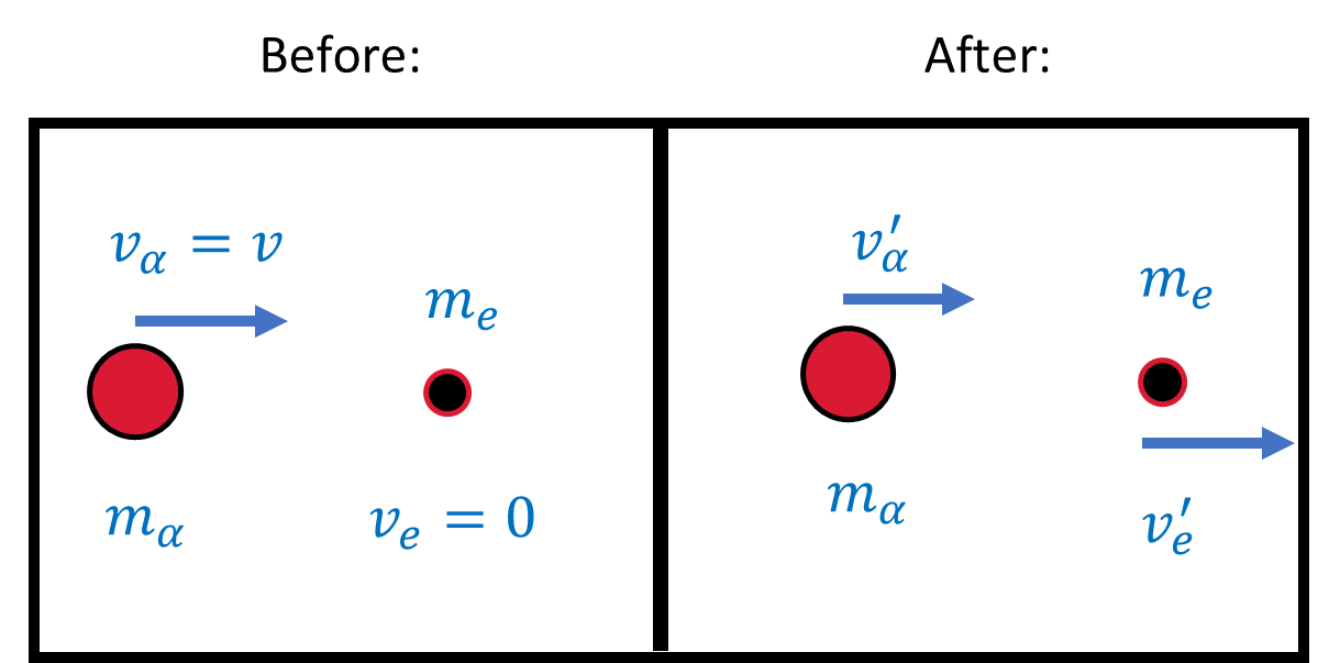
Fig. 4.1 Schematic (before and after) of a collision between an \(\alpha\) particle (with a speed \(v_\alpha\) and mass \(m_\alpha\)) and an electron (with a mass \(m_e\)) initially at rest.

Exercise 4.1

Geiger and Marsden observed backward-scattered \((\theta \geq 90^\circ )\) \(\alpha\) particles when a beam was directed at a piece of gold foil as thin as \(600\ {\rm nm}\). Assuming an \(\alpha\) particle scatters from an electron in the foil, what is the maximum scattering angle?

For particle collisions, we use the conservation of linear momentum and energy. The collision describes an electron (initially at rest) is struck by an \(\alpha\) particle with a velocity \(v\). The maximum scattering angle corresponds to the maximum momentum change for the \(\alpha\) particle, where this transfer occurs when the \(\alpha\) particle hits the electron head-on.

From Fig. 4.1, the conservation of momentum and energy (nonrelativistically) gives

\[ m_\alpha v_\alpha = m_\alpha v_\alpha^\prime + m_e v_e^\prime; \qquad \frac{1}{2}m_\alpha v_\alpha^2 = \frac{1}{2}m_\alpha {v_\alpha^\prime}^2 + \frac{1}{2}m_e {v_e^\prime}^2.\]

From mechanics, a head-on collision with the targe at rest has the following solutions for the final velocities,

\[\begin{split} v_\alpha^\prime = \frac{(m_\alpha - m_e)}{(m_\alpha + m_e)}v_\alpha, \\ v_e^\prime = \frac{2m_\alpha}{(m_\alpha + m_e)}v_\alpha. \end{split}\]

The \(\alpha\) particle is much more massive than the electron (\(m_\alpha/m_e \approx 4\frac{m_p}{m_e} \approx 7000\)). The \(\alpha\) particle’s velocity is hardly affected with \(v_\alpha^\prime \approx v_\alpha\) and the electron’s velocity is nearly \(2v_\alpha\). In general, the maximum momentum change of the \(\alpha\) particle is simply

\[ \Delta \vec{p}_\alpha = m_\alpha \vec{v}_\alpha - m_\alpha \vec{v}_\alpha^\prime = m_e \vec{v}_e^\prime, \]

or for a head-on collision,

\[ \Delta p_{\rm max} = 2m_ev_\alpha.\]

An upper limit for the angular deviation \(\theta\) can be determined by letting \(\Delta p_{\rm max}\) be perpendicular to the initial momentum of the \(\alpha\) particle,

\[ \theta_{\rm max} = \frac{\Delta p_\alpha}{p_\alpha} = \frac{2m_ev_\alpha}{m_\alpha v_\alpha} = \frac{2m_e}{m_\alpha} = \frac{2}{7000}\ {\rm rad} = 0.016^\circ.\]

Thus it is impossible for an \(\alpha\) particle to be deflected through a large angle by a single encounter with an electron.

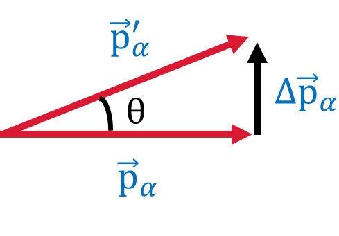
Fig. 4.2 Vector diagram illustrating the change in momentum of the \(\alpha\) particle after scattering from the electron.

What would happen if an \(\alpha\) particle were scattered by many electrons in the target? Multiple scattering is possible, where a calculation for \(N\) random multiple scattering from electrons results in an average scattering angle \(\langle\theta \rangle_{\rm total} \approx \sqrt{N}\theta\). The \(\alpha\) particle ias as likely to scatter on either side for each collision. We can estimate the number of atoms across the thin (\(600\ {\rm nm}\)) gold layer used by Gieger and Marsden by,

(4.1)\[\begin{split} \frac{\text{Number of molecules}}{\rm cm^3} &= N_A \times \text{molar mass} \times \text{density}, \\ &= \left( 6.02 \times 10^{23}\ \frac{\rm molecules}{\rm mol}\right) \left(\frac{1\ {\rm mol}}{197\ {\rm g}}\right) \left( 19.3 \frac{\rm g}{\rm cm^3}\right), \\ &= 5.9 \times 10^{22}\ \frac{\rm molecules}{\rm cm^3} = 5.9 \times 10^{28}\ \frac{\rm atoms}{\rm m^3}. \end{split}\]

If there are \(5.9 \times 10^{28}\ \frac{\rm atoms}{\rm m^3}\), then each atom occupies \((5.9 \times 10^{28})^{-1}\ {\rm m^3}\) of space. Assuming the atoms form a cubic lattice, the distance \(d\) between centers is \(d = (5.9 \times 10^{28})^{-1/3}\ {\rm m} = 2.6 \times 10^{-10}\ {\rm m}\). In the foil, there are

\[ N = \frac{600\ {\rm nm}}{0.26\ {\rm nm}} = 2300\ {\rm atoms} \]

along the \(\alpha\) particle’s path. If we assume the \(\alpha\) particle interacts with one electron from each atom, then

\[ \langle \theta \rangle = \sqrt{2300}(0.016^\circ) = 0.8^\circ, \]

where we used \(theta\) from example above. Even if the \(\alpha\) particle scattered from all 79 electrons in each gold atom, the expected deflection is \(<7^\circ\).

Rutherford proposed that an atom consisted mostly of empty space with a central charge (either positive or negative). In 1911, Rutherford wrote,

“Considering the evidence as a whole, it seems simplest to suppose that the atom contains a central charge distributed through a very small volume, and that the large single deflections are due to the central charge as a whole, and not to its constituents.”

Rutherford worked out the scattering expected for the \(\alpha\) particles as a function of angle, material thickness, velocity and charge. Geiger and Marsden investigated Rutherford’s ideas and confirmed the theory. Rutherford was the first to call the central charged core a nucleus and definitely decided that the core was positively charged, surrounded by the negatively charged electrons.

4.2. Rutherford Scattering

The scattering of charged particles by matter is called Coulomb or Rutherford scattering when it takes place at low energies, where only the Coulomb interactions are important.

A charged particle of mass \(m\), charge \(Z_1e\), and speed \(v_o\) is incident on a target material or scatterer of charge \(Z_2e\). The distance \(b\) denotes the classical impact parameter, which is the closest approach between the beam particle and scatterer (if the projectile had continued in a straight line). The angle \(\theta\) between the incident beam and the deflected particle is called the scattering angle.

Fig. 4.3 The scattering of the alpha particle by the central repulsive Coulomb force leads to a hyperbolic trajectory. From the scattering angle and momentum, one can calculate the impact parameter and closest approach to the target nucleus. Figure credit: Hyperphysics

When the impact parameter is small, the distance of closest approach \(r_{\rm min}\) is small, and the Coulomb force is large. Therefore, the scattering angle is large, and the particle is repelled backward. For large impact parameters, the particles never get close together, so the Coulomb force is small and the scattering angle is also small.

Fig. 4.4 Besides the masses of the target and projectile, the scattering angle depends upon the force and upon the impact parameter. The impact parameter is the perpendicular distance to the closest approach if the projectile were undeflected. Figure credit: Hyperphysics

Rutherford made the following assumptions regarding the relationship between \(b\) and \(\theta\):

1. The scatterer is so massive that it does not significantly recoil; therefore the initial and final kinetic energies of the \(\alpha\) particle are practically equal.

2. The target is so thin that only a single scattering occurs.

3. The bombarding particle and target scatterer are so small that they may be treated as point masses and charges.

4. Only the Coulomb force is effective.

Assumption 1 means that \({\rm K.E._{initial}} \approx {\rm K.E._{final}} \equiv K\) for the \(\alpha\) particle. For central forces like the Coulomb force, the trajectory of the scattered particle lies in a plane due to the conservation of angular momentum \(mv_ob\) defined by the initial velocity \(v_o\).

The instantaneous position of the particle is defined by the angle \(\phi\) and the distance \(r\) from the force center. When the distance \(r\) is a minimum, \(\phi = 0\) and defines the \(z^\prime\) axis. The change in momentum is equal to the impulse

(4.2)\[\Delta \vec{p} = \int \vec{F}_{\Delta p}dt,\]

defined by the force \(\vec{F}_{\Delta p}\) along the direction of \(\Delta \vec{p}\). The massive scatterer absorbs this momentum change without gaining any appreciable kinetic energy (i.e., no recoil). The momentum change is

(4.3)\[\Delta \vec{p} = \vec{p}_f - \vec{p}_i,\]

where the subscripts \(f\) and \(i\) indicate the final and initial momentum, respectively. Since \(p_f \approx p_i\), the vector triangle in Fig. 4.3 is isosceles and the angle \(\theta\) can be bisected. The magnitude of \(\Delta p\) is now

(4.4)\[\begin{align} \Delta p = 2mv_o \sin \frac{\theta}{2}. \end{align}\]

The direction of \(\Delta \vec{p}\) is the \(z^\prime\) axis, where we need to determine the \(z^\prime\) component of \(\vec{F}\). The Coulomb force \(\vec{F}\) is defined as

(4.5)\[\vec{F} = \frac{1}{4\pi \epsilon_o}\frac{Z_1 Z_2 e^2}{r^2}\hat{e}_r,\]

where the unit vector \(\hat{e}_r\) points along a position vector \(\vec{r}\). The component along \(\Delta p\) is given as \(F_{\Delta p} = F \cos \phi\).

Substituting into Eqn. (4.2), we get

\[\begin{align*} \Delta p &= 2mv_o \sin \frac{\theta}{2}, \\ &= \int F\cos \phi dt = \frac{Z_1 Z_2 e^2}{4\pi \epsilon_o}\int \frac{\cos \phi}{r^2} dt. \end{align*}\]

The instantaneous angular momentum must be conserved, so

\[ mr\left(r\frac{d\phi}{dt}\right) = mv_o b, \]

and

\[ r^2 = \frac{v_ob}{d\phi/dt}. \]

Substituting \(r^2\) into the integral for impulse, we get

\[\begin{align*} 2mv_o \sin \frac{\theta}{2} &= \frac{Z_1 Z_2 e^2}{4\pi \epsilon_o} \int \frac{\cos \phi}{v_o b}\frac{dt}{d\phi}dt, \\ &= \frac{Z_1 Z_2 e^2}{4\pi \epsilon_o v_o b} \int_{\phi_i}^{\phi_f} \cos \phi d\phi. \end{align*}\]

If we let the angle \(\phi_i\) be on the negative side and the final angle \(\phi_f\) on the positive side of the \(z^\prime\) axis, then we have \(\phi_i = -\phi_f\), and \(-\phi_i + \phi_f + \theta = \pi\), so \(\phi_i = - (\pi -\theta)/2\) and \(\phi_f = +(\pi - \theta)/2\). Then,

\[ \frac{8\pi \epsilon_o mv_o^2 b}{Z_1 Z_2 e^2} \sin \frac{\theta}{2} = \int_{-(\pi - \theta)/2}^{+(\pi - \theta)/2} \cos \phi d\phi = 2 \cos \frac{\theta}{2}. \]

The impact parameter \(b\) can be determined as

(4.6)\[b = \frac{Z_1 Z_2 e^2}{4\pi \epsilon_o mv_o^2} \cot \frac{\theta}{2} = \frac{Z_1 Z_2 e^2}{8\pi \epsilon_o K} \cot \frac{\theta}{2},\]

where the kinetic energy of the bombarding particle is \(K = mv_o^2/2\). This is the fundamental relationship between the impact parameter \(b\) and the scattering angle \(\theta\) for the Coulomb force.

For a given experiment, we are not able to select individual impact parameters. When we put a detector at a particular angle \(\theta\), we cover a finite \(\Delta \theta\), which corresponds to a range of impact parameters \(\Delta b\). The bombarding particles are incident at varied impact parameters. All the particles with \(b<b_o\) will be scattered at angles \(\theta > \theta_o\). Any particle with an impact parameter inside the area of a circle with an area \(\pi b_o^2\) (i.e., radius \(b_o\)) will be similarly scattered. For Coulomb scattering, the cross section \(\sigma\) is

(4.7)\[\sigma = \pi b^2.\]

The cross section \(\sigma\) is related to the probability for a particle being scattered by the nucleus.

If we have a target foil of thickness \(t\) with \(n\) atoms/volume, the target nuclei per unit area is \(nt\). Because we assumed a thin target area \(A\) and all nuclei are exposed, the number of target nuclei is \(ntA\). The number density \(n\) is related to the density \(\rho\), Avogadro’s number \(N_A\), atoms per molecule \(N_M\), and the molecular weight by

(4.8)\[\begin{align} n &= \rho \left(\frac{\rm g}{\rm cm^3}\right) N_A \left(\frac{\rm molecules}{\rm mol}\right)N_M \left(\frac{\rm atoms}{\rm molecule}\right) \left(M_g ({\rm g/mol})\right)^{-1}, \\ & = \frac{\rho N_A N_M}{M_g} \frac{\rm atoms}{\rm cm^3}. \end{align}\]

Then the number of scattering nuclei per unit area is

(4.9)\[\begin{align} nt = \frac{\rho N_A N_M t}{M_g} \frac{\rm atoms}{\rm cm^2}, \end{align}\]

and the number of target nuclei \(N_s\) is

(4.10)\[\begin{align} N_s = ntA = \frac{\rho N_A N_M tA}{M_g}\ {\rm atoms}. \end{align}\]

The probability of the particle begin scattered is equal number of target nuclei times the cross section divided by the total target area \(A\), or

(4.11)\[\begin{split} f &= \frac{\text{target area exposed by scatterers}}{\text{total target area}} = \frac{ntA\sigma}{A}, \\ &= nt\sigma = nt\pi b^2, \\ &= \pi nt\left(\frac{Z_1Z_2 e^2}{8\pi \epsilon_o K}\right)^2 \cot^2 \frac{\theta}{2}. \end{split}\]

Exercise 4.2

Find the fraction of 7.7-MeV \(\alpha\) particles that is deflected at \(\geq 90^\circ\) from a gold foil of \(1\ {\mu \rm m}\) in thickness.

First, we need the number density \(n\). In The Atomic Models of Thomson and Rutherford, we have already calculated the number density in Eqn. (4.1) so that \(n = 5.9 \times 10^{28}\ \frac{\rm atoms}{\rm m^3}\). To determine fraction \(f\) of alpha particles, we use

\[\begin{align*} f &= \pi nt\left(\frac{Z_1Z_2 e^2}{8\pi \epsilon_o K}\right)^2 \cot^2 \frac{\theta}{2}, \\ &= \pi\left(5.9 \times 10^{28}\ \frac{\rm atoms}{\rm m^3} \right)(10^{-6}\ {\rm m}) \left[\frac{(79)(2)(1.6\times 10^{-19}\ {\rm C})(9\times 10^9\ {\rm N\cdot m^2/C^2})}{2(7.7\times 10^6\ {\rm eV})(1.6 \times 10^{-19}\ {\rm J/eV})} \right]^2 \left(\cot 45^\circ\right)^2, \\ &= 4 \times 10^{-5}. \end{align*}\]

One \(\alpha\) particle in 25,000 is deflected by \(90^\circ\) or greater.

from scipy.constants import e,eV,epsilon_0,pi
import numpy as np

n_au = 5.9e28 #number density of gold atoms per m^3
t_au = 1e-6 #thickness of the gold foil in m
K_alpha = 7.7e6*eV #kinetic energy of the alpha particles in J
Z_au = 79 #number of protons in gold
Z_he = 2 #number of protons in helium
theta_alpha = np.radians(90) #scattering angle of the alpha particles

f_au = pi*n_au*t_au*((Z_au*Z_he*e**2)/(8*pi*epsilon_0*K_alpha))**2/np.tan(theta_alpha/2.)**2

print("The fraction of deflected (7.7 MeV) alpha particles is %1.1e." % f_au)

The fraction of deflected (7.7 MeV) alpha particles is 4.0e-05.

In a typical experiment, a detector is positioned over a range of angles and thus, we need to find the number of particles scattered between \(\theta\) and \(\theta + d\theta\) with corresponding impact parameters (\(b\) and \(b+db\)).

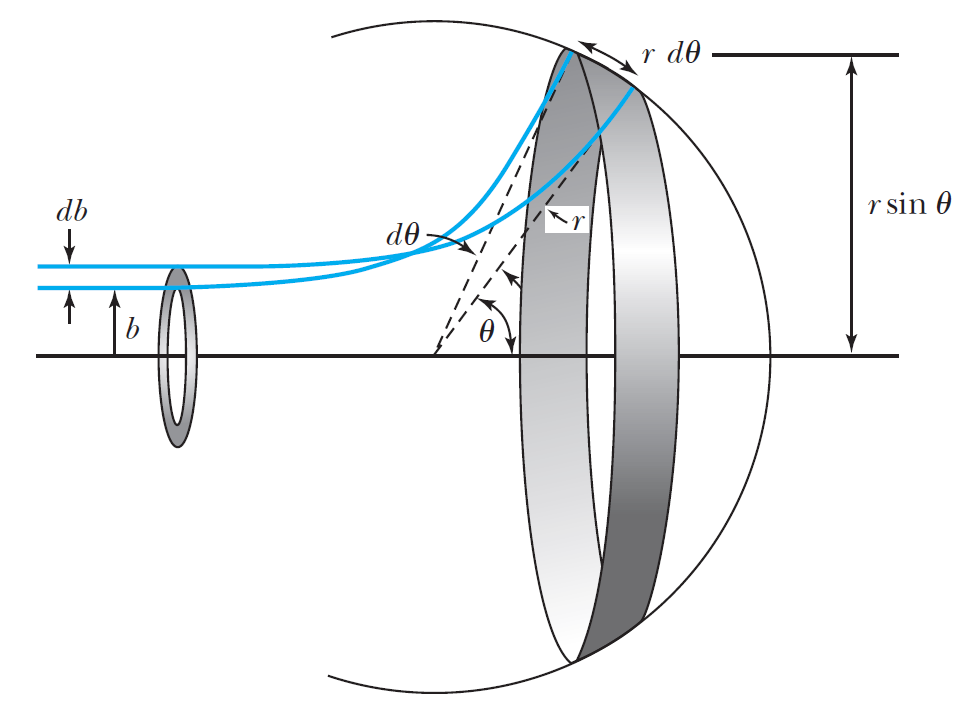
Fig. 4.5 Particles scattered over the range of impact parameters \(b\) corresponding to a range of scattering angles \(\theta\). Image credit: (Thornton & Rex (2012))

The fraction of incident particles scattered is \(df\), or the derivative of Eq. (4.11) with respect to \(d\theta\), is

\[ df = -\pi nt\left(\frac{Z_1Z_2 e^2}{8\pi \epsilon_o K}\right)^2 \cot \frac{\theta}{2} csc^2 \frac{\theta}{2}d\theta. \]

If the total number of incident particles is \(N_i\), the number of particles scattered into the ring of angular width \(d\theta\) is \(N_i|df|\). The area of the ring \(dA\) is \(2\pi r^2 \sin \theta d\theta\). The number of particles scattered per unit area, \(N(\theta)\), into the ring is

(4.12)\[\begin{split} N(\theta) &= \frac{N_i|df|}{dA} = \frac{N_i \pi nt\left(\frac{Z_1Z_2 e^2}{8\pi \epsilon_o K}\right)^2}{2\pi r^2 \sin \theta d\theta} \cot \frac{\theta}{2} csc^2 \frac{\theta}{2}d\theta, \\ &= \frac{N_i nt}{16}\left(\frac{e^2}{4\pi \epsilon_o}\right)^2 \frac{Z_1^2 Z_2^2}{r^2K^2 \sin^4 (\theta/2)}. \end{split}\]

Equation (4.12) is the famous Rutherford scattering equation. The important points are

1. The scattering is proportional to the square of the atomic number of both the incident particle \(Z_1\) and the target scatterer \(Z_2\).

2. The number of scattered particles is inversely proportional to the square of the kinetic energy \(K\) of the incident particle.

3. The scattering is inversely proportional to the 4th power of the \(\sin (\theta /2)\), where \(\theta\) is the scattering angle.

4. The scattering is proportional to the target thickness for thin targets.

Exercise 4.3

Calculate the fraction per \({\rm mm^2}\) area of 7.7-MeV \(\alpha\) particles scattered at \(45^\circ\) from a gold foil of thickness \(0.21\ \mu{\rm m}\) at a distance of \(1\ {\rm cm}\) from the target.

First, we need the number density \(n\). In The Atomic Models of Thomson and Rutherford, we have already calculated the number density in Eqn. (4.1) so that \(n = 5.9 \times 10^{28}\ \frac{\rm atoms}{\rm m^3}\). To determine fraction \(N(\theta)/N_i\) of alpha particles, we use

\[\begin{align*} \frac{N(\theta)}{N_i} & = \frac{nt}{16}\left(\frac{e^2}{4\pi \epsilon_o}\right)^2 \frac{Z_1^2 Z_2^2}{r^2K^2 \sin^4 (\theta/2)}, \\ &= \frac{\left(5.9 \times 10^{28}\ \frac{\rm atoms}{\rm m^3} \right)(2.1 \times 10^{-7}\ {\rm m})\left[(1.6\times 10^{-19}\ {\rm C})^2(9\times 10^9\ {\rm N\cdot m^2/C^2})\right]^2 (2^2) (79^2)}{16(10^{-2}\ {\rm m})^2 (7.7\times 10^6\ {\rm eV})^2(1.6 \times 10^{-19}\ {\rm J/eV})^2 \sin^4 (45^\circ/2) }, \\ &= 0.32\ {\rm m^{-2}} = 3.2 \times 10^{-7}\ {\rm mm^{-2}}. \end{align*}\]

This is the theoretical basis for the experiment performed by Geiger and Marsden to check the validity of Rutherford’s calculation. Our calculated result agrees with their experimental result of \(3.7 \times 10^{-7}\ {\rm mm^{-2}}\) when the experimental uncertainty is taken into account.

from scipy.constants import e,eV,epsilon_0,pi
import numpy as np

n_au = 5.9e28 #number density of gold atoms per m^3
t_au = 2.1e-7 #thickness of the gold foil in m
K_alpha = 7.7e6*eV #kinetic energy of the alpha particles in J
Z_au = 79 #number of protons in gold
Z_he = 2 #number of protons in helium
theta_alpha = np.radians(45) #scattering angle of the alpha particles
r_alpha = 0.01 #distance from the target in m

Ntheta_Ni = n_au*t_au/16.*(e**2/(4*pi*epsilon_0))**2*(Z_au**2*Z_he**2)/(r_alpha**2*K_alpha**2*np.sin(theta_alpha/2.)**4) #fraction per m^2
Ntheta_Ni_mm2 = Ntheta_Ni*(0.001)**2 #convert per m^2 to per mm^2

print("The fraction per mm^2 is %1.2e." % Ntheta_Ni_mm2)

The fraction per mm^2 is 3.15e-07.

4.3. The Classical Atomic Model

Rutherford’s model was generally accepted after experimental verification in 1913, where the atom consisted of a small, massive, positively charged “nucleus” surround by electrons. Thomson’s plum-pudding model was ruled out by the data.

Note

Thomson had previously considered a planetary model resembling the Solar System but rejected it because the planets attract one another while orbiting the Sun, whereas the electrons would repel one another.

Let’s examine the hydrogen atom, which consists of a single proton and electron. Assuming also that the electron has a circular orbit. The force of attraction due to the proton is

(4.13)\[\begin{align} \vec{F}_e = \frac{-1}{4\pi \epsilon_o}\frac{e^2}{r^2}\hat{e}_r, \end{align}\]

where the negative sign indicates the force is attractive. The electrostatic force provides the centripetal force need for the electron to move in a circular orbit at constant speed. Its radial acceleration is

(4.14)\[\begin{align} a_r = \frac{v^2}{r}, \end{align}\]

which depends on the tangential velocity \(v\) of the electron. Newton’s second law gives,

(4.15)\[\begin{align} \frac{1}{4\pi \epsilon_o}\frac{e^2}{r^2} = \frac{m_ev^2}{r}, \end{align}\]

and

(4.16)\[ v = \frac{e}{\sqrt{4\pi \epsilon_o m_e r}}. \]

Exercise 4.4

Are we justified in using a nonrelativistic treatment for the speed of an electron in the hydrogen atom?

We can determine whether special relativity is needed by comparing the nonrelativistic orbital velocity \(v\) to the speed of light \(c\). Typically if \(v/c \lesssim 0.1\), then relativity is not needed (see Section 2.4 for details). The size of the hydrogen atom was thought to be about \(1\ {\rm \unicode{x212B}} = 10^{-10}\ {\rm m}\), so we let \(r = 0.5\ {\rm \unicode{x212B}}\) to estimate the electron’s velocity.

Substituting all the necessary values into Eqn. (4.16), we get

\[\begin{align*} v &\approx \frac{(1.6\times 10^{-19}\ {\rm C}) (9\times 10^9\ {\rm N\cdot m^2/C^2})^{1/2}}{\sqrt{(9.11 \times 10^{-31}\ {\rm kg}})(5 \times 10^{-11}\ {\rm m})}, \\ &\approx 2.2 \times 10^6\ {\rm m/s}, \\ &\approx 7.5 \times 10^{-3}c. \end{align*}\]

This justifies a nonrelativistic treatment.

from scipy.constants import e,c,epsilon_0,m_e
import numpy as np

r_Hyd = 0.5e-10 #approximate radius of the hydrogen atom in m

v = e/np.sqrt(4*np.pi*epsilon_0*m_e*r_Hyd)
print("The approximate orbital velocity of an electron in a hydrogen atom is %1.2e m/s or %1.2e c." % (v,v/c))

The approximate orbital velocity of an electron in a hydrogen atom is 2.25e+06 m/s or 7.51e-03 c.

The kinetic energy of the system due to the electron is \(K = m_ev^2/2\), where we assume that the nucleus is essentially at rest because it is so massive compared with the electron \((m_p/m_e = 1836)\). The potential energy is \(V = -e^2/(4\pi \epsilon_o r)\). The total mechanical energy is

(4.17)\[\begin{align} E = K + V = \frac{1}{2}m_e v^2 - \frac{e^2}{4\pi \epsilon_o r}. \end{align}\]

If we substitute from Eqn. (4.16), then we have

(4.18)\[\begin{split}E &= \frac{1}{2}m_e\left(\frac{e^2}{4\pi \epsilon_o m_e r}\right) - \frac{e^2}{4\pi \epsilon_o r}, \\ &= \frac{e^2}{8\pi \epsilon_o r} - \frac{e^2}{4\pi \epsilon_o r}, \\ &= \frac{-e^2}{8\pi \epsilon_o r}.\end{split}\]

The total energy is negative, which indicates a bound system.

Thus far, the classical (planetary) atomic model seems plausible. The problem arises when we consider that the electron is accelerating due to its motion around the nucleus. From classical electromagnetic theory, an accelerated charge continuously radiates energy in the form of EM radiation.

If the electron is radiating energy, then the total energy \(E\) must decrease continuously, which means that \(r\) must decrease. The electron will continuously radiate energy as the electron orbit becomes smaller and smaller, until the electron crashes into the nucleus! This process would occur in about \(10^{-9}\ {\rm s}\).

4.4. The Bohr Model of the Hydrogen Atom

Shortly after receiving his Ph.D. in 1911, Niels Bohr began traveling and meeting with Thomson, Rutherford, and others. Bohr believed that a fundamental length (\(\sim 10^{-10}\ {\rm m}\)) ws needed for an atomic model and it somehow was connected to Planck’s constant \(h\). Around 1913, Bohr learned of new precise measurements of the hydrogen spectrum and the empirical formulas describing the measurements (e.g., Balmer formula, Rydberg Equation, and Ritz’s combination principles). He set out to develop a fundamental basis to derive them.

Bohr was acquainted with Planck’s work and believed that quantum principles should govern more phenomena than just the blackbody spectrum. He was also impressed with Einstein’s application of the quantum theory to the photoelectric effect and wondered how the quantum theory might affect atomic structure.

In 1913, Bohr published On the Composition of Atoms and Molecules, which laid out his assumptions and was the first step to building his theory. Bohr assumed that electrons moved like planets around a massive, positively charge nucleus, where the electron orbits are circular. The electron has a negative charge \(-e\) and mass \(m\), which revolves around a positive charge \(+e\) of radius \(a\). The central mass is take to be much more massive than the electron such that we can work in its rest frame. The size of the nucleus is small compared with the atomic radius \(a\).

Note

Bohr’s treatment of the atom like a planetary system is a useful fiction, which provides the path to a more sophisticated model that is not intuitive. However, we should remember that analogies are not replacements for an accurate, physical model and not to treat them as such.

Bohr’s model is summarized by the following general assumptions of his 1915 paper:

1. Certain “stationary states” exist in atoms, which differs from the classical stable states. The orbiting electrons do not continuously radiate EM energy. The stationary states are states of definite total energy.

2. The emission (or absorption) of EM radiation can occur in conjunction with a transition between two stationary states. The frequency of the emitted (or absorbed) radiation is proportional to the difference in energy between the two stationary states (1 and 2): \(E = E_1 - E_2 = hf\), and depends on Planck’s constant \(h\).

3. The dynamical equilibrium of the system in the stationary states is governed by the classical laws of physics, but these laws do not apply to transitions between stationary states.

4. The mean value of the kinetic energy \(K\) for the electron-nucleus system is given by \(K = nhf_{\rm orb}/2\) and is dependent on the orbital frequency \(f_{\rm orb}\). For a circular orbit, Bohr pointed out that this assumption is equivalent to the angular momentum of the system in a stationary state is an integral multiple of \(h/(2\pi) = \hbar\) (pronounced “h bar”).

These four assumptions were all Bohr needed to derive the Rydberg equation. Bohr believed that Assumptions 1 and 3 were self-evident because atoms were stable and that the classical laws of physics could not explain the observed behavior of the atom. Bohr later stated (in 1915) that Assumption 2 “appears to be necessary in order to account for experimental facts.” Assumption 4 was the hardest for Bohr’s critics to accept. It is central to the derivation of the binding energy of the hydrogen atom in terms of fundamental constants. Bohr wanted to keep as much of classical physics as possible and only introduced just those new ideas that could explain the experimental data.

Let’s derive the Rydberg equation using Bohr’s assumptions. The total energy (\(K+V\)) of a hydrogen atom was derived in Eqn. (4.18). for circular motion, the magnitude of the angular momentum \(L\) of the electron is

\[ L = |\vec{r} \times \vec{p}| = m_evr. \]

Assumption 4 states this should be

(4.19)\[\begin{align} L = m_evr = n\hbar, \end{align}\]

which is defined by the principal quantum number \(n\) (an integer). Then the equation for the orbital velocity is

(4.20)\[v = \frac{n\hbar}{m_er}.\]

Equation (4.16) provided an independent relation between \(v\) and \(r\). Setting \(v^2\) from Eqn. (4.16) equal to \(v^2\) from (4.20) produces

(4.21)\[v^2 = \frac{e^2}{4\pi \epsilon_o m_e r} = \frac{n^2\hbar^2}{m_e^2}r^2.\]

From Equation (4.21), we can solve for \(r\) in terms of all fundamental constants and the integer \(n\), to get

(4.22)\[r_n = n^2\frac{4\pi \epsilon_o \hbar^2}{m_e e^2} \equiv n^2 a_o,\]

The fundamental constants are grouped into the Bohr radius \(a_o\), which is

\[ a_o = \frac{4\pi \epsilon_o \hbar^2}{m_e e^2} = 0.53 \times 10^{-10}\ {\rm m}. \]

Notice that the smallest diameter of the hydrogen atom is \(2r_1 = 2a_o \approx 10^{-10}\ {\rm m}\), which was the suspected (now known) size of the hydrogen atom!

Bohr found the fundamental length \(a_o\) in terms of fundamental constants (i.e., \(\epsilon_o\), \(h\), \(e\), and \(m_e\)) and the atomic radius is now quantized. The quantization arises from the principal quantum number \(n\), where \(n=1\) represents the lowest energy state, or ground state. The values of \(n>1\) describe the hydrogen atom in an excited state.

The energies of the stationary states \(E_n\) can be determined from Eqns. (4.18) and (4.22) as

(4.23)\[E_n = \frac{-e^2}{8\pi \epsilon_o r_n} = \frac{-e^2}{8\pi \epsilon_o a_o n^2} = -\frac{E_o}{n^2},\]

where the lowest energy state occurs when \(E_1 = -E_o\), and

(4.24)\[E_o = \frac{e^2}{8\pi \epsilon_o a_o} = \frac{e^2}{8\pi \epsilon_o}\frac{m_e e^2}{4\pi \epsilon_o \hbar^2} = \frac{m_e e^4}{32\pi^2 \epsilon_o^2 \hbar^2} = 13.6\ {\rm eV}.\]

Fig. 4.6 The basic hydrogen energy level structure is in agreement with the Bohr model. Common pictures are those of a shell structure with each main shell associated with a value of the principal quantum number \(n\). Figure credit: Hyperphysics

The ground state energy is equivalent to the experimentally measured ionization energy of the hydrogen atom. Bohr’s Assumptions 3 and 4 imply that the atom can exist only in stationary states, or energy levels, with definite, quantized energies \(E_n\). Emission of light occurs when the atom is in an excited state \(n^\prime\) and decays to a lower energy state \(n\). A transition between two levels is described by Assumption 2 as

(4.25)\[\Delta E = hf = E_{n^\prime} - E_n,\]

which depends on the frequency \(f\) of the emitted light (photon). Equation (4.25) can be rewritten in terms of wavelength (\(f=c/\lambda\)) to get the Rydberg Equation by

(4.26)\[\begin{split}f &= \frac{1}{h}(E_{n^\prime} - E_n), \\ \frac{1}{\lambda} &= \frac{-E_o}{hc}\left(\frac{1}{{n^\prime}^2} - \frac{1}{n^2}\right) = \frac{E_o}{hc}\left(\frac{1}{n^2}- \frac{1}{{n^\prime}^2} \right),\end{split}\]

where

(4.27)\[ \frac{E_o}{hc} = \frac{m_e e^4}{64c \epsilon_o^2 \pi^3\hbar^3} = R_\infty. \]

The Rydberg constant \(R_\infty\) is for an infinite nuclear mass and Eqn. (4.26) becomes

(4.28)\[ \frac{1}{\lambda} = R_\infty \left(\frac{1}{n^2}- \frac{1}{{n^\prime}^2} \right), \]

which is similar to Eqn. (3.13). The value of \(R_\infty = 1.097373 \times 10^7\ {\rm m^{-1}}\) agrees well with the experimental value.

Bohr’s model predicts the frequencies (and wavelengths) of the transitions between energy levels in atomic hydrogen. The frequencies of the photons in the emission spectrum of an element are directly proportional to the differences between the energy levels. When we pass white light through hydrogen gas, we find that only the frequencies from an emission spectrum are absent and produce dark lines (i.e., absorption spectrum). In absorption, the electrons within the hydrogen atom move up in energy levels (\(n\rightarrow n^\prime\)) and use particular photon energies to do so.

The atom will remain in an excited state for only a short time \((\sim 10^{-10}\ {\rm s})\) before emitting a photon (in a random direction) and returning to the lower state \(n\). Practically all hydrogen atoms exist in the lowest possible energy state (\(n=1\)), and only the Lyman series absorption lines are observed. These line are not in the visible region. However, the Sun acts as a blackbody (emitting over a broad range of frequencies), where the hydrogen atoms of its outer atmosphere absorb wavelengths of the Balmer series can be seen.

Fig. 4.7 This spectrum was produced by exciting a glass tube of hydrogen gas with about 5000 volts from a transformer. It was viewed through a diffraction grating with 600 lines/mm. The colors cannot be expected to be accurate because of differences in display devices. Figure credit: Hyperphysics

The electron’s velocity in the Bohr model depends on the energy level \(n\) as

(4.29)\[v_n = \frac{n\hbar}{m_e r_n} = \frac{1}{n}\frac{\hbar}{m_e a_o} = \frac{1}{n}\frac{e^2}{4\pi \epsilon_o \hbar}.\]

The velocity of the ground state is \(v_1 = 2.2\times 10^6\ {\rm m/s}\), where the excited states will have lower speeds. Comparing the ground state velocity to the speed of light produces a ratio called the fine structure constant, which is

(4.30)\[\alpha \equiv \frac{v_1}{c} = \frac{e^2}{4\pi \epsilon_o \hbar c} \approx \frac{1}{137}.\]

Exercise 4.5

Determine the longest and shortest wavelengths observed in the Paschen series for hydrogen. Which are visible?

The Paschen series starts with \(n=3\) as its lowest energy state. Looking at Eqn. (4.28), we can see that \(n^\prime = 4\) will give the largest denominator (longest wavelength), and \(n^\prime \rightarrow \infty\) will produce the smallest denominator (shortest wavelength). The wavelength for the transition from \(n= 3\) to \(4\) is determined by:

\[\begin{align*} \frac{1}{\lambda} &= R_\infty\left(\frac{1}{3^2}- \frac{1}{4^2} \right) = \left(1.0974 \times 10^7\ {\rm m^{-1}}\right)\left(\frac{4^2-3^2}{3^2 4^2} \right) = 5.335 \times 10^5\ {\rm m^{-1}}, \\ \lambda &= \frac{1}{5.335 \times 10^5\ {\rm m^{-1}}} = 1.875 \times 10^{-6}\ {\rm m} = 1875\ {\rm nm}. \end{align*}\]

The wavelength for the transition from \(n= 3\) to \(\infty\) is determined by:

\[\begin{align*} \frac{1}{\lambda} &= R_\infty\left(\frac{1}{3^2}- \frac{1}{\infty^2} \right) = \left(1.0974 \times 10^7\ {\rm m^{-1}}\right)\left(\frac{1}{3^2} \right) = 1.219 \times 10^6\ {\rm m^{-1}}, \\ \lambda &= \frac{1}{1.219 \times 10^6\ {\rm m^{-1}}} = 8.203 \times 10^{-6}\ {\rm m} = 820\ {\rm nm}. \end{align*}\]

Both wavelengths are not visible, but in the infrared.

from scipy.constants import Rydberg
import numpy as np

def Rydberg_eqn_Bohr(n,np):
    #calculate the wave number (1/\lambda) for the Rydberg equation using R_infty
    #n = the lower quantum number n
    #np = the higher quantum number np
    return Rydberg*(1./n**2 - 1./np**2) #wave number in m^{-1}

wave_num_max = Rydberg_eqn_Bohr(3,4) #wave number of the Paschen series from 3-->4
lambda_max = 1./wave_num_max #convert wave number to wavelength in m

wave_num_min = Rydberg_eqn_Bohr(3,np.inf) #wave number of the Paschen series from 3-->infinity
lambda_min = 1./wave_num_min #convert wave number to wavelength in m

print("The wave number and wavelength for the 3-->4 transition is %1.3e m^{-1} and %i nm.\n" % (wave_num_max,np.round(lambda_max/1e-9,0)))
print("The wave number and wavelength for the 3-->infinity transition is %1.3e m^{-1} and %i nm.\n" % (wave_num_min,np.round(lambda_min/1e-9,0)))

The wave number and wavelength for the 3-->4 transition is 5.334e+05 m^{-1} and 1875 nm.

The wave number and wavelength for the 3-->infinity transition is 1.219e+06 m^{-1} and 820 nm.

4.4.1. The Correspondence Principle

In the early 20th century, physicists had trouble reconciling classical and quantum results. For example, there were two radiation laws: one used in classical electrodynamics and another was expressed in Bohr’s atomic model. Physicists proposed several correspondence principles to relate the classical and quantum results. In 1913, Bohr proposed the best correspondence principle, which is

In the limits where classical and quantum theories should agree, the quantum theory must reduce to the classical result.

—Bohr’s correspondence principle

Consider the predictions of the two radiation laws. The frequency of the radiation produced by the atomic electrons in the Bohr model should agree with the predictions from classical electrodynamics where the Planck’s constant is unimportant (i.e., for large quantum number \(n\)). Classically, the frequency of emitted radiation is equal to the electron’s orbital frequency \(f_{\rm orb}\) around the nucleus:

(4.31)\[\begin{align} f_{\rm classical} &= f_{\rm orb} = \frac{\omega}{2\pi} = \frac{v}{2\pi r},\\ &= \frac{1}{2\pi}\sqrt{\frac{e^2}{4\pi \epsilon_o m_e r^3}}, \\ & = \frac{1}{n^3}\frac{m_e e^4}{4\epsilon_o^2 h^3}. \end{align}\]

Substituting values in terms of fundamental constants from Bohr’s model leads to a classical frequency that depends on the principal quantum number \(n\). Starting from the Bohr model, the nearest we can come to continuous radiation is a cascade of transitions from a \(n+1\) level to the \(n\) level. The frequency of the transition from \(n+1 \rightarrow n\) is

(4.32)\[\begin{split}f_{\rm Bohr} &= \frac{E_o}{h}\left[ \frac{1}{n^2} - \frac{1}{(n+1)^2} \right],\\ &= \frac{E_o}{h}\left[\frac{(n+1)^2 - n^2}{n^2(n+1)^2} \right], \\ &= \frac{E_o}{h}\left[\frac{2n+1}{n^2(n+1)^2} \right].\end{split}\]

For large \(n\), Eqn. (4.32) becomes

\[ f_{\rm Bohr} \approx \frac{E_o}{h}\left[ \frac{2n}{n^4} \right] = \frac{2E_o}{hn^3}. \]

If we substitute Bohr’s \(E_o\) from Eqn. (4.24), the result is

(4.33)\[\begin{align} f_{\rm Bohr} = \frac{1}{n^3}\frac{m_e e^4}{4\epsilon_o^2 h^3} = f_{\rm classical}. \end{align}\]

The frequencies of the radiated energy agree between the classical theory and the Bohr model for large values of the principle quantum number \(n\). Bohr’s correspondence principle is verified for large electron orbits, where classical and quantum physics should agree.

4.5. Success and Failures of the Bohr Model

4.5.1. Reduced Mass Correction

The electron and hydrogen nucleus actually revolve about their mutual center of mass, where this is a two-body problem. Instead of just \(r\), we should have used the electron’s distance \(r_e\) and the nucleus’ distance \(r_{\rm nucleus}\) from the center of mass. A straightforward analysis from classical mechanics shows that the two-body problem can be reduced to an equivalent one-body problem in terms of the reduced mass \(\mu_e\) that is moving around the center of mass. The reduced mass depends on the mass of the nucleus \(M\) and the electron mass \(m_e\), or

(4.34)\[\begin{align} \mu_e = \frac{m_eM}{m_e + M} = \frac{m_e}{1+m_e/M}. \end{align}\]

In the case of the hydrogen atom, the mass of the nucleus \(M\) is the proton mass, and the correction for the hydrogen atom is \(\mu_e = 0.999456\ m_e\). Athough it is small, the difference is still measurable experimentally. The Rydberg constant \(R_\infty\) (see (4.27)) should be replaced by

(4.35)\[ R = \frac{\mu_e}{m_e}R_\infty =\frac{\mu_e e^4}{64c \epsilon_o^2 \pi^3\hbar^3}. \]

Using the reduced mass for hydrogen, the Rydberg constant is \(R_{\rm H} = 1.096776 \times 10^6\ {\rm m^{-1}}\).

Exercise 4.6

Calculate the wavelength for the \(3\rightarrow 2\) transition (called the \({\rm H_\alpha}\) line) for the hydrogen, deuterium, and tritium atom.

We need to determine the correct \(R\) for each atom, where the required masses are

\[\begin{align*} \text{Proton} &= 1.007276\ {\rm u}\\ \text{Deuteron} &= 2.013553\ {\rm u}\\ \text{Triton (tritium nucleus)} &= 3.015500\ {\rm u}\\ \text{electron} &= 0.0005485799\ {\rm u}. \end{align*}\]

The respective corrected values for \(R\) (see Eqn. (4.35)) are

\[\begin{align*} R_H &= \frac{0.0005485799\ {\rm u}}{1.007276\ {\rm u}}R_\infty = 0.99946R_\infty, \\ R_D &= \frac{0.0005485799\ {\rm u}}{2.013553\ {\rm u}}R_\infty = 0.99973R_\infty, \\ R_T &= \frac{0.0005485799\ {\rm u}}{3.015500\ {\rm u}}R_\infty = 0.99982R_\infty. \end{align*}\]

The calculated wavelength for the \({\rm H_\alpha}\) line is

\[\begin{align*} \lambda = R^{-1}\left(\frac{2^23^2}{3^2-2^2}\right) =7.2R^{-1}, \\ \lambda\text{(hydrogen)} = 656.47\ {\rm nm}, \\ \lambda\text{(deuterium)} = 656.29\ {\rm nm},\\ \lambda\text{(tritium)} = 656.23\ {\rm nm}. \\ \end{align*}\]

Deuterium was discovered when two closely spaced spectral lines of hydrogen near \(656.4\ {\rm nm}\) wer observed in 1932. These proved to be the \({\rm H_\alpha}\) lines of atomic hydrogen and deuterium. Tritium \(^{3}{\rm H}\) contains 1 proton and 2 neutrons within its nucleus.

from scipy.constants import physical_constants,m_e,Rydberg
import numpy as np

#Rydberg = R_infty

m_p = physical_constants['proton mass in u'][0] #mass of proton in u
m_D = physical_constants['deuteron mass in u'][0] #mass of deuteron in u
m_T = physical_constants['triton mass in u'][0] #mass of triton in u
m_e = physical_constants['electron mass in u'][0] #mass of deuteron in u

atom = ['Hydrogen', 'Deuterium','Tritium']
m_nucleus = [m_p,m_D,m_T]
for i in range(0,3):
    mu = m_e/(1+m_e/m_nucleus[i])
    R = (mu/m_e)*Rydberg
    l_alpha = 7.2/R/1e-9
    print("The corrected Rydberg constant for %s is %1.5f R_infty.\n" % (atom[i],R/Rydberg))
    print("The H_alpha wavelength for %s is %3.2f nm.\n" % (atom[i],l_alpha))

The corrected Rydberg constant for Hydrogen is 0.99946 R_infty.

The H_alpha wavelength for Hydrogen is 656.47 nm.

The corrected Rydberg constant for Deuterium is 0.99973 R_infty.

The H_alpha wavelength for Deuterium is 656.29 nm.

The corrected Rydberg constant for Tritium is 0.99982 R_infty.

The H_alpha wavelength for Tritium is 656.23 nm.

The Bohr model may be applied to any single-electron atom even if the nuclear charge is greater than 1 proton charge \((+e)\) (e.g., \({\rm He^+}\) and \({\rm Li^{2+}}\)). The only change needed is in the calculation of the Coulomb force, where \(e^2\) is replace with \(Ze^2\) to account for the nuclear charge of \(+Ze\). The Rydberg Equation becomes

(4.36)\[ \frac{1}{\lambda} = Z^2R \left(\frac{1}{n^2} - \frac{1}{{n^\prime}^2}\right). \]

4.5.2. Other Limitations

With increased precision in optical spectrographs, (two lines that were originally believed to be a single line) could be resolved and is known as fine structure. Arnold Sommerfeld adapted the special theory of relativity to Bohr’s hypotheses and accounted for some ot the “splitting” of spectral lines. In addition, external magnetic (Zeeman effect) and electric (Stark effect) fields applied to radiating atoms affected the spectral lines by splitting and broadening them. Classical electromagnetic theory could explain the (normal) Zeeman effect, but it was unable to account for the Stark effect.

The Bohr model was a great step forward, but it had its limitations:

1. It could be successfully applied only to single-electron atoms.

2. It was not able to account for the intensities or the fine structure of the spectral lines.

3. Bohr’s model could not explain the binding of atoms into molecules.

The Bohr model was a theory to explain the hydrogen spectral lines, but it doesn’t correctly describe atoms in general. Despite its flaws, Bohr’s model should not be denigrated. It was a step along the path to the correct quantum explanation.

4.6. Characteristic X-Ray Spectra and Atomic Number

With the initial success of the Bohr’s model, it was believed tha the general characteristics fo the Bohr-Rutherford atom would prevail. We can now understand the characteristic x-ray wavelengths by adopting Bohr’s electron shell hypothesis. Bohr’s model suggests that an electron shell is quantified by a radius \(r_n\) that is associated with the principal quantum number \(n\). Electrons with lower values of \(n\) are more tightly bound to the nucleus (i.e., stronger Coulomb force). The radii of the electron orbits increase in proportion to \(n^2\), where a specific energy is also linked to each value of \(n\). We may assume that the inner electron shells (low values of \(n\)) are filled before outer shells as electrons are added.

Fig. 4.8 The x-rays emitted between different atomic states. The Greek letter subscripts indicate the value of \(\Delta n\), where the Roman letter denotes the value of \(n\). Image credit: OpenStax: University Physics Vol 3.

Historically the electron shells were given letter names starting from \(K\) for \(n=1\), \(L\) for \(n=2\), and so on. Atomic nuclei with a larger positive charge require and equal number of electrons to remain electrically neutral. We may suppose that heavy atoms with many electrons contain many electrons within several shells. What happens when a high-energy electron in an x-ray tube collides with one of the \(K\)-shell electrons in a target atom?

If enough energy is supplied to the \(K\) electron to dislodge (free) it from the atom, then a vacancy is left in the \(K\) shell. This allows another electron to descend from a higher energy level and fill the vacancy so that the ground state is full. In the process, the electron has to emit some radiation to transition downward. When this occurs, we call the EM radiation an x-ray and it has the energy

\[ E\text{ (x-ray)} = E_{n^\prime} - E_n, \]

where the process is precisely analogous to what happens in an excited hydrogen atom (see Eqn. (4.25)). The photon produced when the electron falls from the \(L\) (\(n=2\)) shell into the \(K\) (\(n=1\)) shell is called a \(K_\alpha\) x-ray. When it falls from a higher level, like \(M\) (\(n=3\)), it is called a \(K_\beta\) x-ray. The relative positions of the energy levels of the various shells differ for each element (i.e., differing amount of positive charge in the nucleus), and the characteristic x-ray energies are simply the energy difference between the shells.

Physicists in Rutherford’s lab had already fully accepted the concept of the atomic number and most European physicists believed that the atomic weight \(A\) was an important factor in the structure of the periodic table of elements. The atomic number \(Z\) is the number of protons (positive charges) in the nucleus, where the actual makeup of the nucleus was unknown at the time. In 1913, Henry Moseley was working in Rutherford’s laboratory and was engaged in cataloguing the characteristic x-ray spectra of a series of elements. Moseley compared the frequencies of the characteristic x-rays with atomic number of the elements. He found empirically that the frequency and atomic number were related by

(4.37)\[f_{K_\alpha} = \frac{3}{4}cR\left(Z-1\right)^2.\]

The empirical relation holds for the \(K_\alpha\) x-rays and a similar result was found for the \(L\) shell.

Note

Moseley began his work in 1913 and completed his work in 1914. It is clear that Bohr and Moseley discussed physics and even corresponded after Bohr left for Copenhagen. But, Moseley does not mention Bohr’s model in his 1914 paper. It is not known to what extent Bohr’s ideas had any influence Moseley’s work.

Fig. 4.9 Moseley’s data indicating the relationship between the atomic number \(Z\) and the characteristic x-ray frequencies. Image credit: OpenStax: University Physics Vol 3.

If a vacancy occurs in the \(K\) shell, then there is still one electron remaining in the \(K\) shell. An electron in the \(L\) shell will feel an effective charge of \((Z-1)e\) due to the \(+Ze\) from the nucleus and \(-e\) from the remaining \(K\) shell electron. The other electrons outside the \(K\) shell hardly affect the \(L\) shell electron. The x-ray produced when a transition occurs from the \(n=2\rightarrow 1\) shell has the wavelength (from Eqn. (4.36)) of

(4.38)\[\begin{align} \frac{1}{\lambda_{K_\alpha}} &= (Z-1)^2 R\left(\frac{2^2 -1^2}{1^22^2}\right), \\ &= \frac{3}{4}R(Z-1)^2, \\ f_{K_\alpha} &= \frac{c}{\lambda_{K_\alpha}} = \frac{3}{4}cR(Z-1)^2. \end{align}\]

Moseley’s equation describing the \(K_\alpha\) shell x-rays is an application of Bohr’s model. The general form for the \(K\) series of x-ray wavelengths is

(4.39)\[\begin{align} \frac{1}{\lambda_K} &= R(Z-1)^2 \left(\frac{n^2 -1}{n^2}\right). \end{align}\]

Moseley correctly concluded that the atomic number \(Z\) was the determining factor for the ordering of the periodic table, where the reordering by atomic number was more consistent with chemical properties than one based on atomic weight. He also concluded that the atomic number of an element should be identified with the number of positive charges (protons) in the nucleus. He tabulated all the atomic numbers between aluminum \({\rm Al}\ (Z=13)\) to gold \({\rm Au}\ (Z=79)\) and pointed out that there were still three elements (\(Z=43,\ 61,\ \text{and } 75\)) yet to be discovered! The element promethium (\(Z=61\)) was discovered around 1940.

Moseley’s research helped put the Rutherford-Bohr model on a firmer footing. It clarified the importance of the electron shells for all the elements (not just for hydrogen). It also helped to show that the atomic number was the significant factor in the ordering of the periodic table, not the atomic weight.

Exercise 4.7

Moseley found experimentally an equation describing the frequency of the \(L_\alpha\) line as \(f_{L_\alpha} = (5/36)cR(Z-7.4)^2\). How can the Bohr model explain this result? What is the general form for the \(L\) series wavelengths \(\lambda_L\)?

The \(L_\alpha\) x-ray results from the transition of \(n=3\rightarrow 2\), where the \(L\) series refer to transition to the \(n=2\) state from higher states. For the case of the \(K\) series, the effective charge of the nucleus \(Z_{\rm eff}\) was simply \(Z-1\). Since we don’t yet know the detailed arrangement of electrons, we just let \(Z=Z_{\rm eff}\) and its value will be determined empirically. From Bohr’s model we can proceed to find

(4.40)\[\begin{align} f_{L_\alpha} = cRZ_{\rm eff}^2\left(\frac{3^2-2^2}{2^23^2}\right) = \frac{5}{36}cRZ_{\rm eff}^2. \end{align}\]

According to Moseley’s data, the effective charge must be \(Z-7.4\). We can rewrite our result by replacing \(3\rightarrow n\) (and changing to wavelength) to get

(4.41)\[\begin{align} \frac{1}{\lambda_L} = RZ_{\rm eff}^2\left(\frac{n^2 -4}{4n^2}\right) = R(Z - 7.4)^2\left(\frac{n^2 -4}{4n^2}\right). \end{align}\]

4.7. Atomic Excitation by Electrons

So far quantum theory has been characterized by the packets of electromagnetic radiation that we call photons (or quanta). The Bohr model explained the measured optical spectra of certain atoms. Spectroscopic experiments were performed by exciting the elements (e.g., a high-voltage discharge tube to examine the emission spectra).

In 1914, James Franck and Gustav Hertz decided to study the possibility of transferring a part of an electron’s kinetic energy to an atom (i.e., the Franck-Hertz experiment). Their measurements would provide a new technique for studying atomic structure. In their experiment, electrons are emitted thermionically from a hot cathode (filament) and are accelerated by an electric field. After passing through a wire mesh, the electrons are subjected to a decelerating voltage (\(\sim 1.5\ {\rm V}\)) between the mesh and an anode (collector). If the electrons have \(>1.5\ {\rm eV}\) after passing through the mesh, then they will have enough energy to reach the collector and be registered as current through and electrometer (i.e., an extremely sensitive ammeter). A voltmeter measures the accelerating voltage \(V\), where the final result shows the collector current as a function of the measured voltage.

Fig. 4.10 Photograph of a vacuum tube used for the Franck–Hertz experiment in instructional laboratories. There is a droplet of mercury inside the tube, although it is not visible in the photograph. C - cathode assembly; the cathode itself is hot, and glows orange. It emits electrons which pass through the metal mesh grid (G) and are collected as an electric current by the anode (A). Figure credit: Wikipedia.

The accelerating electrons pass through a region containing mercury (\(\rm Hg\)) vapor. Franck and Hertz found the electrons did not lose energy as long as the accelerating voltage \(V < 5\ {\rm V}\) (i.e., the maximum kinetic energy of the electrons was \(<5\ {\rm eV}\)). The electron current measured in the electrometer increased with a larger voltage, but there was a sudden drop in the current when the accelerating voltage increased above \(5\ {\rm V}\). As the accelerating voltage increased, the measured current increased again until the voltage reached \(10\ {\rm V}\), which it suddenly dropped. Franck and Hertz interpreted this behavior ast teh onset of ionization of the \({\rm Hg}\) atom (i.e., freeing an electron from \({\rm Hg}\)). They later realized that the \({\rm Hg}\) atom was actually begin excited to its first excited state.

Fig. 4.11 Anode current (arbitrary units) versus grid voltage (relative to the cathode). This graph is based on the original 1914 paper by Franck and Hertz. Image credit: Wikipedia.

Within the context of Bohr’s picture of quantized atomic energy levels, the ground state \(E_o\) is when all the electrons are in their lowest possible energy states. The first excited state has an energy \(E_1\) and is measured using the ground state energy \(E_o\) as the “zero point” (i.e., \(E_o = 0\)). The energy difference between states is called the excitation energy. The first excited state of \({\rm Hg}\) is at \(4.88\ {\rm eV}\) and as long as the accelerating electron’s kinetic energy is below \(4.88\ {\rm eV}\), then no energy can be transferred to the recoil of \({\rm Hg}\) atom.

For an accelerating voltage below \(4.88\ {\rm V}\), the collision between the electron and the \({\rm Hg}\) atom is elastic, where the electron can only bound off the \(\rm Hg\) atom with the same kinetic energy. Above \(4.88\ {\rm V}\), the collision becomes inelastic, where the electron can promote the \(\rm Hg\) atom to its first excited state. A bombarding electron that has lost energy in an inelastic collision then has too little energy to reach the collector. Above \(4.88\ {\rm V}\), the current dramatically drops. The process can repeat gain when the accelerating voltage increases to \(9.8\ {\rm V}\ (\approx 2\times 4.88\ {\rm V})\), where a second electron is excited and the current drops sharply again.

The Franck-Hertz experiment convincingly proved the quantization of atomic electron energy levels. The bombarding electron’s kinetic energy can change only by discere amounts. They performed the experiment with gases of several other elements and obtained similar results.

4.8. Homework Problems

Problem 1

Calculate the impact parameter for scattering a \(7.7\ \rm MeV\ \alpha\) particle from gold at an angle of (a) \(1^\circ\) and (b) \(90^\circ\).

Problem 2

Compute and compare the electrostatic and gravitational forces in the classical hydrogen atom, assuming a radius of \(5.3 \times 10^{-11}\ {\rm m}\).

Problem 3

A hydrogen atom in an excited state absorbs a photon of wavelength \(410\ {\rm nm}\). What where the initial and final states of the hydrogen atom?

Problem 4

A hydrogen atom exists in an excited state for typically \(10^{-8}\ {\rm s}\). How many revolutions would an electron make in an \(n=3\) state before decaying?

Problem 5

Calculate the Rydberg constant for the single-electron (hydrogen-like) ions of helium, potassium, and uranium. Compare each of them with \(R_\infty\) and determine the percentage difference.

Problem 6

What wavelengths for the \(L_\alpha\) lines did Moseley predict for the missing \(Z= 43,\ 61,\ \text{and}\ 75\) elements (See Exercise 4.7)?

Problem 7

Calculate the \(K_\alpha\) and \(K_\beta\) wavelengths for \(\rm He\) and \(\rm Li\).

Problem 8

The redshift measurements of spectra from magnesium and iron are important in understanding distant galaxies. What are the \(K_\alpha\) and \(L_\alpha\) wavelengths for magnesium and iron?

Problem 9

A beam of \(8.0\ \rm MeV\ \alpha\) particles scatters from a gold foil of thickness \(0.32\ \rm \mu m\).

(a) What fraction of the \(\alpha\) particles is scattered between \(1.0^\circ-2.0^\circ\)?

(b) What is the ratio of \(\alpha\) particles scattered through angles greater than \(1^\circ\) to the number scattered through angles greater than \(10^\circ\)?