Galactic Evolution
Contents
6. Galactic Evolution#
6.1. Interactions of Galaxies#
6.1.1. Evidence of Interactions#
Nearly all galaxies belong to clusters, and the galaxies take up a larger fraction of the cluster’s volume than do stars in a stellar cluster. The spacing between galaxies is typically only \(100\times\) larger than the size of the galaxies themselves.
Densely populated clusters (e.g., the Coma cluster) have a higher proportion of elliptical galaxies (i.e., early-type) in their center than they do in their outer, less dense regions. The central regions of these rich, regularly shaped clusters also have a higher proportions of ellipticals than the centers of less populated, amorphous irregular clusters (e.g., Hercules cluster). These observations seem to correlate with the increased probability of interactions and/or mergers between galaxies in regions of higher galaxy number density. Interactions tend to increase the velocity dispersions of stars within each of the galaxies involved, which could possibly destroy disk structures in spiral (late-type) galaxies and cause the galaxies to relax to early-type \(r^{1/4}\) profiles.

Fig. 6.1 This false-color mosaic of the central region of the Coma cluster (width \({\sim}1^\circ\)) combines infrared and visible-light images to reveal thousands of faint objects (green). Follow-up observations showed that many of these objects, which appear here as faint green smudges, are dwarf galaxies belonging to the cluster. The mosaic combines visible-light data from the Sloan Digital Sky Survey (color coded blue) with long- and short-wavelength infrared views (red and green, respectively) from NASA’s Spitzer Space Telescope. Image Credit: Wikipedia:Coma_Cluster; NASA / JPL-Caltech / L. Jenkins (GSFC).#
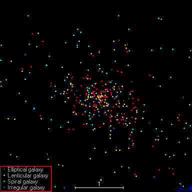
Fig. 6.2 This map has a width of four degrees, where the blue points show the spiral galaxies and irregular galaxies. Image Credit Atlas Map of the Universe.#
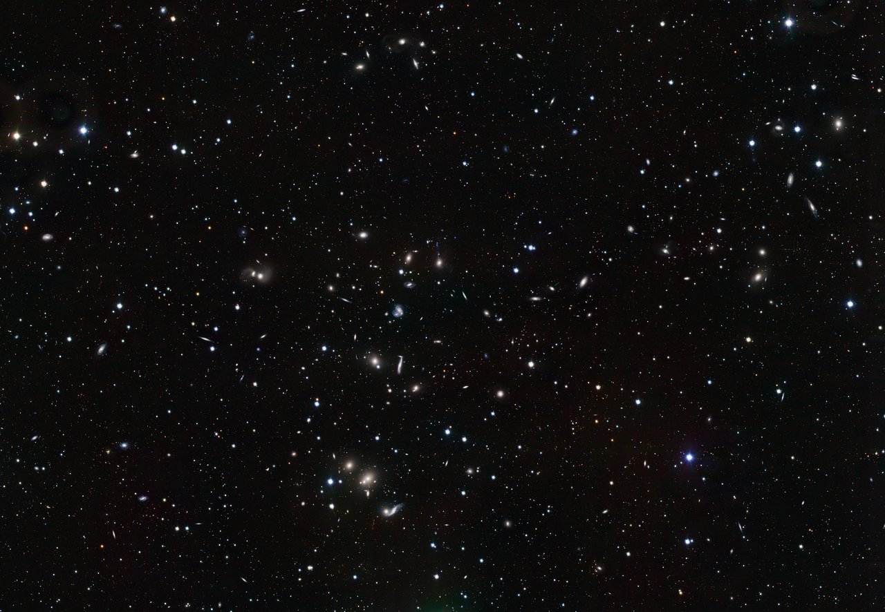
Fig. 6.3 Image of a wide variety of interacting galaxies in the young Hercules galaxy cluster taken with the Very Large Telescope (VLT) Survey Telescope. Image Credit ESO/INAF-VST/OmegaCAM.#
A VLA radio survey of the H I layer of galactic disks found that at least \(50\%\) of all disk galaxies display warped disks. Also, more than half of all ellipticals harbor discrete shells of stars (see Binney (1992) and Hernquist (1992) for more details). Some disk warping may be due to tidal interactions with smaller satellite galaxies and shells in ellipticals are signatures of mergers.
Observations suggest that hot, X-ray emitting gas occupies much of the space between galaxies in rich clusters and has a mass equal to (or exceeding) the mass of all the cluster’s stars. It seems that the gravitational influence of interacting galaxies is largely responsible for removing the gas from the individual galaxies that make up the cluster, while still leaving the gas trapped in the cluster’s gravitational well. Only a small fraction of the galaxies’ gas is removed in a direct collision, where mergers may initiate a burst of star formation that produces stellar mass loss and supernovae. This can also lead to a galactic superwind capable of liberating a large amount of gas.
This evidence suggests that interactions between galaxies play an important role in their evolution. In the hierarchical “bottom-up” scenario of galaxy formation, large galaxies are formed by mergers and the gravitational capture of smaller entities. In this view, the interactions seen today between galaxies are simply a natural extension of their formative years.

Fig. 6.4 The plumes on the opposite sides of NGC 520 are evidence of a tidal interaction possibly ending in the merger of the two colliding galaxies. Image Credit NASA, ESA, the Hubble Heritage Team (STScI/AURA)-ESA/Hubble Collaboration and B. Whitmore (STScI).#
6.1.2. Dynamical Friction#
What happens when galaxies collide? Given that stars are generally spread very far apart in galaxies, the change of even single stellar collision is quite small. Instead, interactions between stars will be gravitational in nature.
Imagine that an object (e.g., a globular cluster or small galaxy) of mass \(M\) is moving through an infinite collection of stars, gas clouds , and dark matter with a constant density \(\rho\).
Assumption: The mass of each object in the background “sea” of material is much less than \(M\), so \(M\) continues to move in a straight line instead of being deflected.
In the absence of collisions, \(M\) might move unimpeded. But, as \(M\) moves forward the other objects are gravitationally pulled toward its path, with the closest ones feeling the largest force.
This produces a region of enhanced density along the path, with a high-density “wake” trailing \(M\). The net gravitational force on \(M\) that opposes its motion is called dynamical friction.
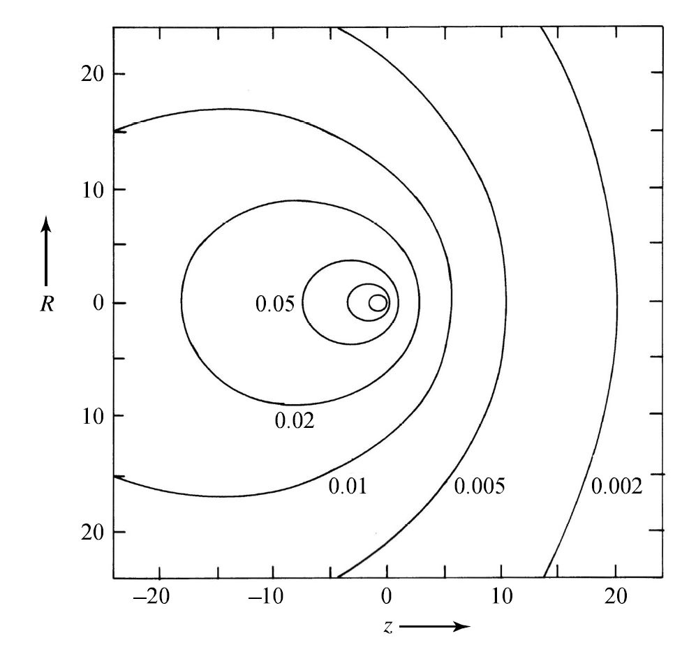
Fig. 6.5 The fractional enhancement in the density of stars caused by the motion a a mass \(M\) in the positive \(z\) direction. Image Credit: Carroll & Ostlie (2007); Figure adapted from Mulder (1983).#
Kinetic energy is transferred from \(M\) to the surrounding material as the speed of \(M\) is reduced.
The physical quantities involved in dynamical friction are the mass \(M\), the speed \(v_M\) of the massive object, and the mass density \(\rho\) of the surrounding material. AS a result, the expression for the force must contain \(GM\), \(v_M\), and \(\rho\) only. The expression for the force of dynamical friction is will have the following form,
where \(C\) is dimensionless, but not a constant. It is a function that depends on how \(v_M\) compares with the velocity dispersion \(\sigma\) of the surrounding medium (see Binney & Tremaine (1987) for more details). For \(v_M \sim 3\sigma\), the typical values of $C are
23 for the LMC,
76 for globular clusters, and
160 for ellipticals.
Clearly the dynamical friction must be proportional to the mass density of stars. Assuming that the relative numbers of objects of various objects don’t change, doubling \(\rho\) means doubling the number of objects and would double the gravitational force on \(M\).
The mass \(M\) itself is squared, where one power comes from its role in producing the high-density wake that trails behind it and the other from the gravitational force on \(M\) produced by the enhanced density.
Consider the velocity squared term in the denominator. If \(M\) moves twice as fast, it will spend only half as much time near a given object. The impulse \((\int \mathbf{F}dt = \Delta \mathbf{p})\) given to that object is only half as great. Consequently, the density enhancement develops only half as rapidly, and \(M\) will be twice as far away by the time the enhancement arises. Thus, slow encounters are much more effective at decreasing the speed of an intruding mass.
To get an estimate of the timescale associated with the effects of dynamical friction acting on a galaxy’s globular clusters, recall that flat rotation curves imply that the density of the dark matter halo may be approximated simply by,
Substituting this density into the equation for the dynamical friction \(f_d\) results in,
If the cluster’s orbit is circular with a radius \(r\), then its orbital angular momentum is \(L = M v_M r\). Since dynamical friction acts tangentially to the orbit and opposes the cluster’s motion, a torque of magnitude \(\tau = rf_d\) is exerted on the cluster. The torque reduces the cluster’s angular momentum according to
A flat rotation curve implies that the orbital speed \(v_M\) is essentially constant. Thus differentiating the angular momentum and substituting for the torque gives,
Separating the variables and integrating produces an expression that describes the time required \(t_c\) (i.e., cluster lifetime) for the globular cluster to spiral into the center of the host galaxy from an initial radius \(r_i\), or
Solving for the cluster lifetime yields
This expression can be inverted to find the most distant cluster that could have been captured (via dynamical friction) within the estimated age of the galaxy:
Exercise 6.1
Consider a globular cluster that orbits the Andromeda galaxy (M31). Assume that the cluster’s mass is \(M = 5 \times 10^6\ M_\odot\) and its velocity is \(v_m = 250\ \rm km/s\), which is typical for the rotation curve in the outer part of the galaxy. The age of M31 is approximately \(13\ \rm Gyr\).
What is the maximum distance from the center that the globular cluster could have originated (assuming only inspiral from dynamical friction)?
Since we are looking for the maximum distance, the value of \(t_{\rm max} = 13\ {\rm Gyr} = 1.3\times 10^{10}\ {\rm yr}\). The typical value for \(C\) is \(76\) in globular clusters. Thus, we find (after converting to appropriate units)
Similar mass clusters in M31 that were within approximately \(4\ \rm kpc\) of the center of the galaxy would have spiraled into its nucleus by now. The maximum radius \(r_{\max} \propto \sqrt{M}\), which implies that globular clusters with \(M > 5\times 10^6\ M_\odot\) could have been gathered from greater distances. This may explain why there are not any very massive globular clusters remaining around M31 today.
from scipy.constants import G, parsec
import numpy as np

M_sun = 1.989e30 #mass of Sun in kg
sec2yr = 3600*24*365.25

t_max = 1.3e10*sec2yr #Age of M31 in sec
C = 76 #constant for globular clusters
M = 5e6*M_sun #mass of globular cluster in M_sun (to kg)
v_M = 250e3 #rotation speed of globular cluster in m/s

r_max = np.sqrt(C*t_max*G*M/(2*np.pi*v_M)) #maximum radius in m
r_max /= parsec

print("The maximum radius of the globular cluster is %1.2f kpc." % (r_max/1000))
The maximum radius of the globular cluster is 3.72 kpc.
Not only are globular clusters affected by dynamical friction but so are satellite galaxies. A stream of material has been tidally stripped from the Magellanic Clouds. It appears that dynamical friction will ultimately cause the Magellanic Clouds to merge with the Milky Way some \(14\ \rm Gyr\) in the future. This is a fate already suffered by the Sagittarius dSph galaxy, which is a remnant of the dwarf galaxy in Canis Major and possibly a progenitor galaxy of \(\omega\) Cen.
The process of satellite accretion has a variety of possible consequences. The gravitational torques involved in the merger of a satellite galaxy in a retrograde orbit could produce the counter-rotating cores that are observed in some elliptical galaxies. In a disk galaxy, mergers may excite global oscillation modes and are capable of producing the featureless disks that are characteristic of Ir (amorphous) galaxies.
6.1.3. Rapid Encounters#
In contrast to the slow encounters via dynamical friction are rapid encounters that occur so quickly between two galaxies that their stars do not have time to respond. Even in the special case where two galaxies pass through one another, there is no significant dynamical friction because there is no appreciable density enhancement.
In this impulse approximation, the stars barely have time to alter their positions. As a result, the internal potential energy \(U\) of each galaxy is unchanged by the collision. However, the gravitational work that each galaxy performs on the other has increased the internal kinetic energies of both galaxies in a random way. This internal kinetic energy comes at the expense of the overall kinetic energies of the galaxies’ motions with respect to one another.
The amount of internal energy gained by galaxies depends on the proximity of the approach \(r_{\rm min}\) of the galaxies involved, with energy declining rapidly from more distant encounters (\(E \propto 1/r_{\rm min}^4\)).
Suppose that one of the galaxies gains some internal kinetic energy during the interaction. To determine how it will respond, assume that the galaxy was initially in equilibrium, which means that the virial theorem was applicable prior to the encounter and its initial kinetic, potential, and total energies were related by \(2K_i = -U_i = -2E_i\).
Imagine that during the encounter the galaxy’s internal kinetic energy increased by \(\Delta K\). Since the potential energy has remained essentially remained constant, that means the galaxy’s total energy has to increase by the same factor \(\Delta K\), or \(E_f = E_i + \Delta K\). As a result, the galaxy has been thrown out of virial equilibrium. After a few orbital periods, the equilibrium can be re-established, and then the final kinetic energy must be (according to the virial theorem)
As equilibrium is regained, the internal kinetic energy of the galaxy actually decreases by \(2\Delta K\) from the value it had just after the collision.
How does the galaxy accomplish this reduction?
It can regain equilibrium by converting excess kinetic energy into an increased (i.e., less negative) gravitational potential energy. The galaxy expands slightly as the separation between its masses increases.
It can reduce the kinetic energy by the most energetic components carrying it out away from the galaxy in the form of stars and gas. This evaporation cools the galaxy and moves it towards a new equilibrium.
Both of these processes may occur, where the specific circumstances of the collision will determine which one dominates. For example, a high-speed, nearly head-on collision may produce a ring galaxy (e.g., the Cartwheel galaxy).
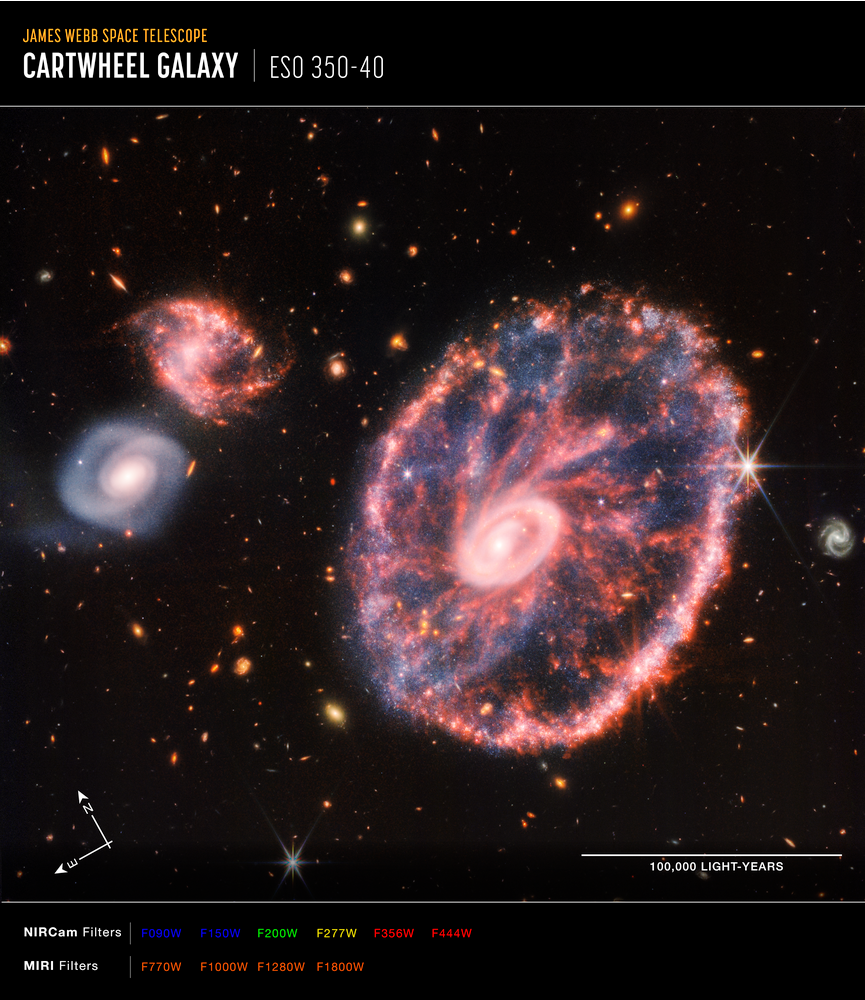
Fig. 6.6 This image of the Cartwheel and its companion galaxies is a composite from Webb’s Near-Infrared Camera (NIRCam) and Mid-Infrared Instrument (MIRI), which reveals details that are difficult to see in the individual images alone. This galaxy formed as the result of a high-speed collision that occurred about 400 million years ago. The Cartwheel is composed of two rings, a bright inner ring and a colorful outer ring. Both rings expand outward from the center of the collision like shockwaves. Image Credit: NASA, ESA, CSA, STScI, Webb ERO Production Team#
If two galaxies are gravitationally bound to ne another, they will eventually merge given enough time. Galaxies do not follow the same trajectories as if they were point masses because of their extended mass distributions. Some orbital energy is diverted into increasing the galaxies’ internal energy, and the orbit shrinks a bit. Tidal forces may also dissipate the orbital energy by pulling stars and gas out of one or both galaxies, which is known as tidal stripping.
The python code below produces a figure for point masses in a circular orbit, where it contains valuable insights for the present case of extended galaxies in non-circular orbits. In particular, the tidal radii \(\ell_1\) and \(\ell_2\) are the distances from the center of each galaxy to the inner Lagrange point \(L_1\). As the two galaxies move about one another, the shape of the equipotential surfaces and the values of the tidal radii are constantly changing. If stars or clouds of gas extend beyond a galaxy’s tidal radius, they have an tendency to escape from the gravitational well. As a result, the density of galactic material undergoes a sharp decline beyond the tidal radius.
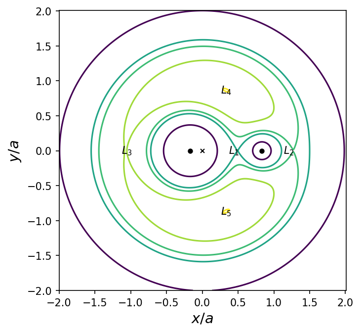
Fig. 6.7 Equipotentials for \(M_1 = 0.85\ M_\odot\), \(M_2 = 0.17\ M_\odot\), and \(a=0.178\ R_\odot\). The axes are in units of \(a\) with the system’s center of mass (\(\times\)) at the origin. The equipotential curves \(\Phi\) are normalized in units of \(G(M_1 + M_2)/a = v_{\rm circ}^2\), where the values are \(-2.5\) (purple), \(-1.875\) (forest green), \(-1.768\) (the dumbbell; green), \(-1.583\) (light green), and \(-1.431\) (the \(L_4\) and \(L_5\) points; yellow-green). The collinear points \(L_1\), \(L_2\), and \(L_3\) are labeled, along with dots representing the point masses.#
import matplotlib.pyplot as plt
import numpy as np
from myst_nb import glue

#Restricted Three Body Problem Psuedopotential contours
#see Musielak & Quarles (2014); https://ui.adsabs.harvard.edu/abs/2014RPPh...77f5901M/abstract
#see Solar System Dynamics; Murray & Dermott (2000)

def eff_grav_pot(M_1,M_2,x,y):
    r_sqr = x**2 + y**2
    s_1 = np.sqrt((x-x_1)**2+y**2)
    s_2 =  np.sqrt((x-x_2)**2+y**2)
    phi = -G*(M_1/s_1 + M_2/s_2) - 0.5*omega_sqr*r_sqr
    return phi/v_M_sqr

def plot_Lagrange(Lx,Ly,lbl):
    ax.text(Lx,Ly,lbl,fontsize=10,horizontalalignment='center',verticalalignment='center')

R_sun = 0.00465047 # radius of the Sun in AU
G = 4*np.pi**2

M_1 = 0.85 # mass of star 1 in M_sun
M_2 = 0.17 # mass of star 2 in M_sun
mu = M_2/(M_1+M_2) #mass ratio of M_1 and M_2
alpha = 1-mu
a = 0.718*R_sun #semimajor axis of binary in AU
omega_sqr = G*(M_1+M_2)/a**3 #squared mean motion of the binary (2*pi/P)^2
v_M_sqr = G*(M_1+M_2)/a

x_1 = -mu*a #x-position to the left of the center of mass for mass 1
x_2 = alpha*a #x-position to the right of the center of mass for mass 2

phi_loc = np.round(np.array([-2.5,-1.875,-1.768,-1.583,-1.431]),3)
Hill = (M_2/(3*M_1))**(1./3.)
L_1 = x_2*(1 - Hill - Hill**2/3 - Hill**3/9.)
L_2 = x_2*(1 + Hill + Hill**2/3 - Hill**3/9.)
L_3 = x_1 - x_2*(1+(5./12)*(M_2/M_1)-(5./12)*(M_2/M_1)**2)
L_4x, L_4y = 0.5-mu, np.sqrt(3)/2.
L_5x, L_5y = 0.5-mu, -np.sqrt(3)/2.


fig = plt.figure(figsize=(5,5),dpi=150)
ax = fig.add_subplot(111)

x_coord = np.arange(-2,2.01,0.001)*a
y_coord = np.arange(-2,2.01,0.001)*a
X,Y = np.meshgrid(x_coord,y_coord)
Z = eff_grav_pot(M_1,M_2,X,Y)

CS = ax.contour(X/a,Y/a,Z,levels=phi_loc)

ax.plot(x_1/a,0,'k.',ms=8)
ax.plot(x_2/a,0,'k.',ms=8)
ax.plot(0,0,'kx',ms=4)

plot_Lagrange(L_1/a,0,"$L_1$")
plot_Lagrange(L_2/a,0,"$L_2$")
plot_Lagrange(L_3/a,0,"$L_3$")
plot_Lagrange(L_4x,L_4y,"$L_4$")
plot_Lagrange(L_5x,L_5y,"$L_5$")

ax.set_xlabel("$x/a$",fontsize=14)
ax.set_ylabel("$y/a$",fontsize=14)

glue("Lagrange_points_fig", fig, display=False);
Polar-ring galaxies and dust-lane ellipticals are normal galaxies that are orbited by rings of gas, dust, and stars that were stripped from other galaxies as they passed by or merged. Polar rings contain \(10^9\ M_\odot\) (or more) of gas and are found only around elliptical or S0 galaxies. It is estimated that \({\sim}5%\) of all S0 galaxies have (or did have in the past) a polar ring.
Fig. 6.8 The polar-ring galaxy NGC 4650A. Image Credit: Hubble Heritage Team (AURA/STScI/NASA)#
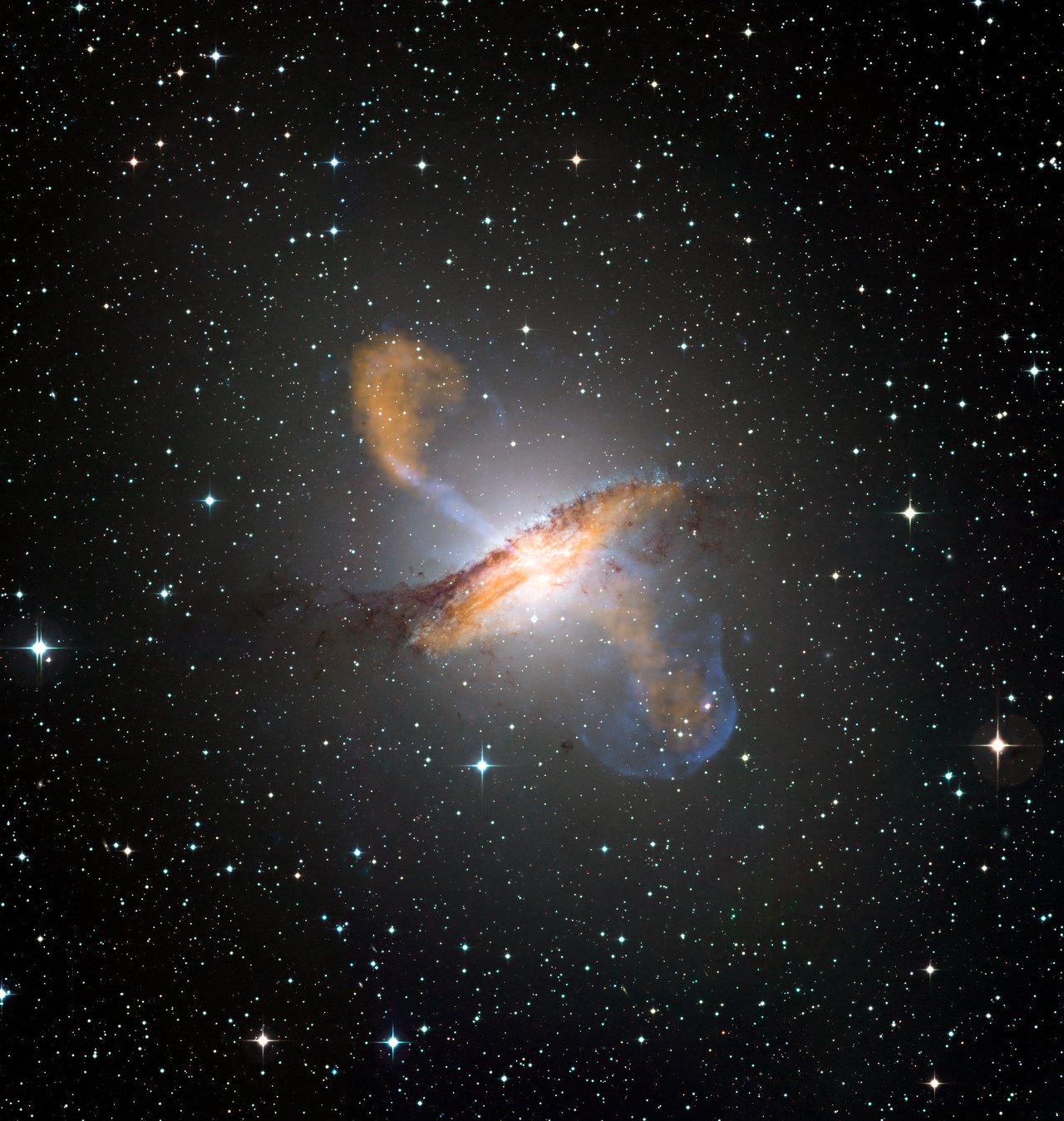
Fig. 6.9 Color composite image of Centaurus A (NGC 5128), revealing the lobes and jets emanating from the active galaxy’s central black hole. Image Credit: ESO/WFI (Optical); MPIfR/ESO/APEX/A.Weiss et al. (Submillimetre); NASA/CXC/CfA/R.Kraft et al. (X-ray)#
Because the rings respond to the gravitational field of the galaxies, astronomers use them as probes of the 3D distribution of matter (both luminous and dark) in their host galaxies. The results of studying several polar-ring galaxies show that they are surrounded by spherical dark halos. An example of a well-known dust-lane elliptical is Centaurus A (NGC 5128), which is also a powerful radio source. An extreme case of a gaseous ring (no stars) is that one that encircles the central two galaxies of the M96 group in the constellation Leo. The gas is in an elliptical orbit around the two galaxies, where the eccentricity is \(e=0.402\).
An elliptical orbit is the result of an inverse-square law force, which means that the gas in the M96 group must lie beyond andy dark matter halos surrounding the two galaxies. The semimajor axis of the orbit is \(a = 101\ \rm kpc\), so the maximum extent of any dark halo must be given by \(r_p = a(1-e) = 60\ \rm kpc\), the perigalacticon distance. This calculation must be viewed cautiously because the ring is merely a locus of gas and may not in fact coincide with the orbit followed by a single particle.
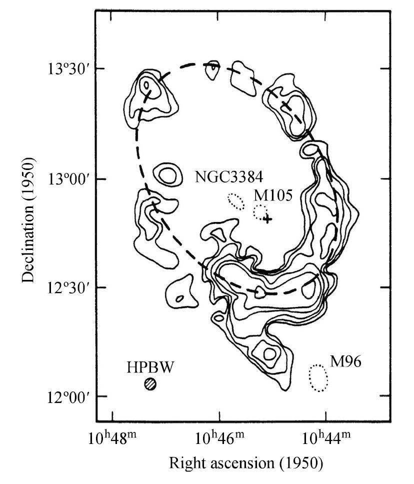
Fig. 6.10 21-cm radio contours showing the ring of neutral hydrogen around the galaxies M105 and NGC 3384 in the M96 group. Image Credit: Carroll & Ostlie (2007); Figure adapted from Schneider (1991)#
6.1.4. Modeling Interactions with \(N\)-Body Simulations#
The simulation of only 3 bodies interacting through gravity is complicated and couldn’t be solved (even by Newton). The merger of two galaxies cannot be solved analytically, where numerical solutions are necessary.
If the relative speed of the galaxies is substantially greater than the velocity dispersions of their stars, the collision will not result in a merger.
If the relative speed of the collision is less than the velocity dispersion of the stars in one of the galaxies, a merger is inevitable.
The situation is particularly complicated when the relative velocity of the galaxies is comparable to the velocity dispersion of stars in one of the galaxies. This situation is best studied by numerical experiments involving *\(N\)-body simulations similar to the ones used to investigate the bar instability in a disk of stars. In these computations, Newton’s second law is used to follow the motions of the stars through a sequence of time intervals.
One of the first numerical experiment considered a galaxy as a massive nucleus surrounded by concentric rings of disk stars (see Toomre & Toomre (1972) for more details). To simplify the calculations, the stars in the disk were allowed to feel the gravitational pull of the galactic nuclei, but not each other. The Toomre brothers (Alar & Juri Toomre) succeeded in demonstrating how interactions could explain the appearance of galaxies like M51 (the Whirlpool), which has a bridge of stars and gas that appears to extend to its neighbor galaxy NGC 5195. In addition, The Toomres were successful in reproducing the appearance of tidal-tail galaxies (e.g., NGC 4038 and NGC 4309; the “Antennae”).
The above simulation evaluates the interactions between two galaxies as they pass by each other. The simulation contains 5000 Stars, the galaxies are simulated as scaled down version. The initial conditions resemble the Whirlpool Galaxy although no physical data from this galaxy was used in the simulation (courtesy of Ingo Berg using the Barnes-Hut Galaxy Simulator).
Only close, slow encounters produce bridges and tails. The effect is most pronounced when the orbital angular speed of one of the galaxies matches the angular speed of some of the stars in the other galaxy’s disk. The resulting orbital resonance (which acts on both the near and far sides of the disk) allows the tidal forces to be especially effective. Two bulges tend to develop on opposite sides of one (or both) of the galaxies, similar to Earth’s tidal bulges.

Fig. 6.11 The NASA/ESA Hubble Space Telescope has snapped the best ever image of the Antennae Galaxies. Image Credit: Wikipedia:Antennae_Galaxies; ESA/Hubble/NASA#
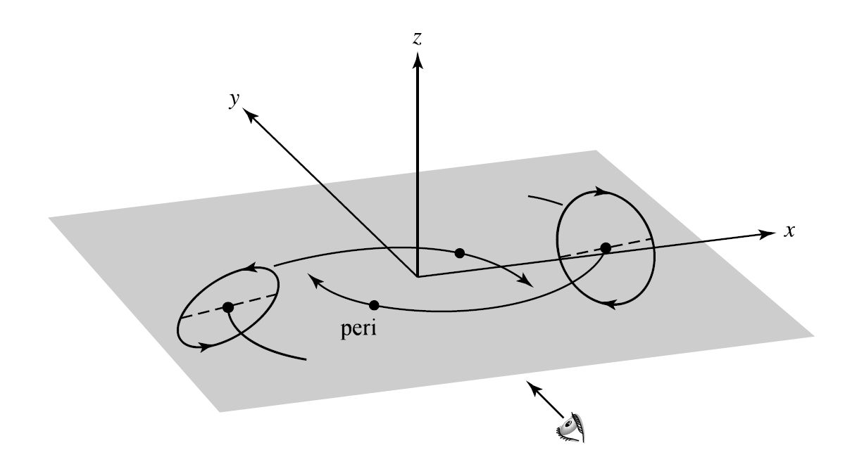
Fig. 6.12 The orbital geometry used to calculate the formation of the tidal-tail galaxies, NGC 4038 and NGC 4309. Image Credit: Carroll & Ostlie (2007); Figure adapted from Barnes (1988)#
Tidal stripping pulls out streams of stars and gas as the two galaxies dance around one another. When conditions are right, the stars and gas torn from the near side will form an apparent bridge, while the material stripped from the far side moves off to form a curving tail due to angular momentum conservation.
Modern computer codes include the effects of dark matter and gravitational interactions (i.e., self-gravity) of individual stars and gas clouds. These codes have also been used to simulate the merger of a disk galaxy (with a central bulge and halo) and a satellite galaxy with \(10\%\) of the mass of the primary. The presence of a dark matter halo significantly decreases the timescale of a merger because it allows the galaxies to interact over much larger distances. The satellite is devoured and absorbed in only two revolutions of the disk galaxy.
Roughly 1/2 of the stars in the Milky Way’s outer stellar halo move in retrograde orbits, which is probably a consequence of tidal stripping and/or mergers of other dwarf galaxies. There are two different spatial distributions of globular clusters around the Milky Way. The inner clusters are old and vary little in age, while the outer population has a wider spread in age. The inner clusters also tend to have a preferential direction for their Galactic orbits, while the outer clusters have randomly oriented orbits. It appears likely that these outer clusters formed elsewhere and were captured later by the Milky Way.
If a satellite galaxy is moving at an angle with respect to the plane of the disk, the merger can result in a warped disk that persists for \(3-5\) billion years. More than \(50\%\) of the galactic disks (including the Milky Way) display a warp in their gas distributions and most of these galaxies do not appear to have nearby companions. The absence of a companion might argue in favor ofa merger, under the assumption that the companion was enveloped by the primary galaxy. However, most disk show no explicit evidence that a merger has occurred.
6.1.5. Starburst Galaxies#
Larson & Tinsley (1974) found that strongly interacting galaxies tend to be bluer than isolated ones of the same type. They attributed the excess blue light to hot, newborn stars and argued that tidal interactions have induced vigorous bursts of star formation in these galaxies. The increased luminosity is difficult to detect because it is shrouded in thick clouds of gas and dust, like all star formation. the light emitted by the young stars at visible and UV wavelengths is absorbed and re-radiated in the IR.
In 1983, the Infrared Astronomy Satellite (IRAS) found that these starburst galaxies are extremely bright at IR wavelengths, pouring out up to \(98\%\) of their energy in this portion of the spectrum. In comparison, the Milky Way emits \(30\%\) of its luminosity in the IR, while M31 emits only a few percent.
Most of the star formation is confined within \({\sim}1\ \rm kpc\) of the galaxy’s center, where radio telescopes have detected vast clouds containing \(10^9-10^{12}\ M_\odot\) of hydrogen gas that serves as fuel. Between \(10-300\ M_\odot\) of gas is converted into stars each year in a starburst galaxy, while only \(2-3\) stars are formed annually in the Milky Way. The clouds typically contain sufficient H to support this star formation rate for \({\sim}10^8-10^9\ \rm yr\), although a given burst may last for only \({\sim}20\ \rm Myr\).
Since hydrogen clouds were initially distributed throughout the galactic disk, one puzzle is how a violent interaction with another galaxy could have removed \(>90\%\) of the clouds’ angular momentum, allowing the gas to become concentrated in the galactic center. An answer may be found through numerical simulations of colliding galaxies, where such studies indicate that the gas and stars react differently to the impact of an intruding galaxy.
The gas tends to move out in front of the stars as they orbit the galactic center. The stars’ gravity then pulls back on the gas, the resulting torque on the gas reduces its angular momentum, and this reduction of angular momentum causes the gas to plunge toward the galactic center. As the two galaxies begin to merge, more angular momentum is lost. Shock fronts then compress the gas, and a burst of star formation begins.

Fig. 6.13 This mosaic image of the magnificent starburst galaxy, M82 (NGC 3034) is the sharpest wide-angle view ever obtained of M82. It is a galaxy remarkable for its webs of shredded clouds and flame-like plumes of glowing hydrogen blasting out from its central regions where young stars are being born 10 times faster than they are inside in our Milky Way Galaxy. Image Credit: NASA, ESA and the Hubble Heritage Team (STScI/AURA).#
From the unusual appearance of M82 (NGC 3034), astronomers thought that this galaxy was exploding. The current interpretation is that between \(10^7-10^8\ \rm yr\) ago, the inner \(400\ \rm pc\) of M82 began a tremendous episode of star formation that is still continuing. The center of M82 contains a wealth of OB stars and supernova remnants that have expelled more than \(10^7\ M_\odot\) of gas from the plane of the galaxy. All of this violent activity may have been triggered by a tidal interaction with M81 (a spiral galaxy that is now about \(36\ \rm kpc\) away from M82) and linked by a gaseous bridge of neutral hydrogen. The center of M81 is known to be a significant source of X-rays, with an X-ray luminosity \(L_X = 1.6 \times 10^{33}\ \rm W\). It has been suggested that M81 has a central black hole that is begin “fed” by infalling gas at the rate of \(10^{-5}-10^{-4}\ M_\odot/{\rm yr}\).
6.1.6. Mergers in Elliptical and cD Galaxies#
The importance of interactions in galactic evolution is most obvious for elliptical galaxies. The cD galaxies are typically found at the centers of rich, regular clusters. More than half of the known cD galaxies have multiple nuclei that move differently than the galaxy as a whole. Although the typical orbital speed of a star in a cD galaxy is \({\sim}300\ \rm km/s\), the multiple nuclei move with relative velocities of \({\sim}1000\ \rm km/s\). All of this is taken as evidence that cD galaxies are the products of galactic merger that supplied the multiple nuclei and expansive halo of stars. Their frequent occurrence at the bottom of a cluster’s gravitational potential well makes collisions and other close encounters all the more probable.
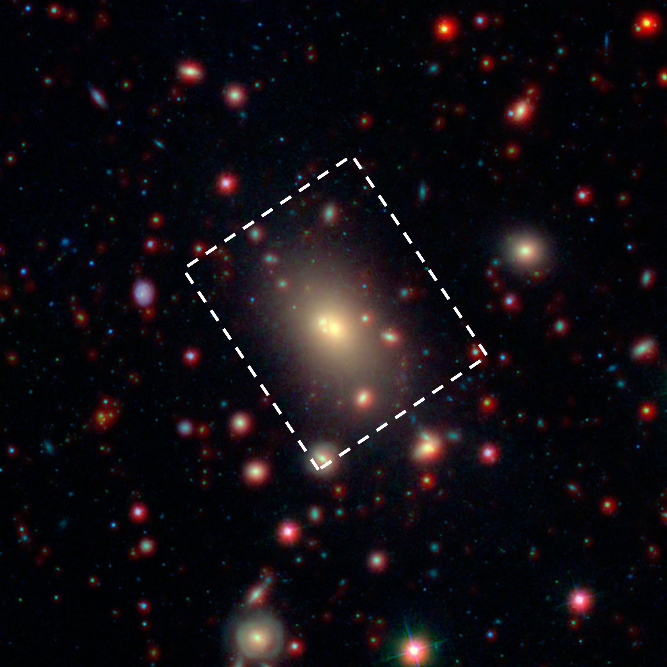
Fig. 6.14 The passage of three small galaxies through a giant elliptical in the cluster Abell 2199 (center of white rectangle). The galaxy cluster was observed by NASA’s Wide-field Infrared Survey Explorer (WISE) and Spitzer Space Telescope missions. Image Credit: Wikipedia:Abell_2199; NASA/JPL-Caltech/SDSS/NOAO.#

Fig. 6.15 The glowing object in this Hubble Space Telescope image is an elliptical galaxy called NGC 3923. It is located over 90 million light-years away in the constellation of Hydra. NGC 3923 is an example of a shell galaxy where the stars in its halo are arranged in layers. Finding concentric shells of stars enclosing a galaxy is quite common and is observed in many elliptical galaxies. Image Credit: ESA/Hubble & NASA.#
Normal elliptical galaxies show evidence of interactions and mergers, particularly the boxy galaxies. About \(25\%\) of all ellipticals have very different velocity fields in their cores when compared with their outer regions. Observations also reveal that \(56\%\) of all ellipticals have faint shells (as do \(32\%\) of all S0 galaxies). Otherwise normal ellipticals may have as many as 20 large concentric arcs of very low surface brightness, both outside and inside the galaxy.
Numerical experiments find that the concentric shells may be the result of head-on (or nearly head-on) collisions with smaller galaxies that have only a few percent of the mass of the larger elliptical. The captured stars slosh back and forth in the elliptical’s gravitational well, like water rocking back and forth in a large bowl. Arcs are seen where the stars slow and reverse their courses. The natural spread in the stellar kinetic and potential energies create the concentric arcs.
6.1.7. Binary Supermassive Black Holes#
An intriguing consequence of the merging of two large galaxies is the apparently inevitable formation of a binary system of supermassive black holes, whether they are ellipticals or spirals. If each galaxy involved in the merger originally contained a supermassive black hole, the two black holes would migrate toward the center of the potential well of the combined system as a direct result of dynamical friction.
Depending on their trajectories, the two black holes would probably enter into a well-separated binary system. One such system appears to be NGC 6420, which has two very strong X-ray sources that are currently separated by a distance of about \(1\ \rm kpc\).

Fig. 6.16 These images taken with Hubble, Keck, and Pan-STARRS telescopes reveal the final stage of a union between pairs of galactic nuclei in the messy cores of colliding galaxies. Image Credit: Wikipedia:NGC_6240; NASA, ESA, and M. Koss (Eureka Scientific, Inc.); Hubble image: NASA, ESA, and M. Koss (Eureka Scientific, Inc.); Keck images: W. M. Keck Observatory and M. Koss (Eureka Scientific, Inc.); Pan-STARRS images: Panoramic Survey Telescope and Rapid Response System and M. Koss (Eureka Scientific, Inc.).#
As the two supermassive black holes orbit around one another, they will have a profound and disturbing time-dependent gravitational influence on stars near the center of the merged galaxy. As with other three-body systems where one member is less massive than the other two (i.e., restricted three-body problem), it is probable that individual stars will be ejected from the central region of the galaxy.
If the total mass of stars ejected in this way becomes comparable to the mass of the black holes, enough angular momentum and energy will be carried away by the stars that the two black holes will spiral toward one another. When the black holes become sufficiently close, they will produce large amounts of gravitational radiation that will further rob them of the energy and angular momentum needed to stay separated. The final outcome of the process will be a merger of the two black holes, producing an even larger beast in the center of the merged galaxy.
6.2. The Formation of Galaxies#
6.2.1. The Eggen, Lynden-Bell, Sandage (ELS) collapse model#
Eggen, Lynden-Bell, & Sandage (1962) presented an important early attempt at modeling the Milky Way’s evolution, which is now called the ELS collapse model. Their work was based on observed correlations between the metallicity of stars in the solar neighborhood with their orbital eccentricities and angular momenta. Eggen, Lynden-Bell, and Sandage noted that
the most metal-poor stars tend to have the highest eccentricities, the largest \(w\) components of their peculiar motions, and the lowest angular momenta about the rotation axis of the Galaxy.
the metal-rich stars tend to exist in nearly circular orbits and are confined to regions near the Galactic plane.
To explain the kinematic and chemical properties of stars within the solar neighborhood, ELS suggested that the Milky Way formed from the rapid collapse of a large proto-Galactic nebula. The oldest halo stars formed early in the collapse process while still on nearly radial trajectories, which resulted in their highly elliptical orbits above and below the Galactic plane.
As a further consequence of their rapid formation, the model predicts that the halo stars are naturally very metal-poor (i.e., Pop II) since the ISM had not yet had time to be enriched by stellar nucleosynthesis. The ISM evolved chemically over time as the first generations of massive stars generated heavier elements in their interiors, underwent supernova explosions, and ejected metal-rich material back into the ISM.
The model predicts that the rapid collapse slowed when collisions between gas and dust particles became more frequent and the kinetic energy of infall was dissipated (i.e., converted into thermal energy). The presence of angular momentum in the original proto-Galactic nebula meant that the cloud began to rotate more quickly as the radius decreased. The combination of the increased dissipation and the increased speed let to the development of chemically enriched gas from which Pop I stars continue to form today.
Exercise 6.2
The free-fall collapse time required for the proto-Galactic cloud can be estimated using concepts from homologous collapse. Assume that the proto-Galactic cloud contained some \(5\times 10^{11}\ M_\odot\), which is the estimated mass of the Milky Way Galaxy within a nearly spherical volume of radius \(50\ \rm kpc\) and includes the dark matter halo.
What is the estimate for the free-fall time using homologous collapse?
Looking back at Chapter 12 from Carroll & Ostlie (or the Chapter 12 Notes) on star formation, we find that the free-fall time depends solely on the initial density \(\rho_o\). The initial density can be estimated as
assuming that the mass was uniformly distributed over the sphere. With \(\rho_o\), we can then calculate the free-fall time \(t_{\rm ff}\) as
If the nebula were initially centrally condensed, the inner portions of the Galaxy would collapse more rapidly than the outer, rarefied regions. This may explain the existence of the very old stellar population within the bulge. The high metal abundance of bulge stars would arise if the first, massive (short-lived) stars could quickly enrich the relatively dense ISM in that part of the Galaxy.
Recall that the lifetimes of the most massive stars are \({\sim}1\ {\rm Myr}\), which is much shorter than the estimated free-fall timescale.
from scipy.constants import G, parsec
import numpy as np

M_sun = 1.989e30 #mass of Sun in kg
sec2yr = 3600*24*365.25 #number of seconds in a year
M = 5e11*M_sun #mass of Milky Way with a radius of 50 kpc
r = 5e4*parsec

rho_o = M/(4/3.*np.pi*r**3)
print("The initial density rho_o is %1.2e kg/m^3." % rho_o)
print("---------------")
t_ff = np.sqrt(3*np.pi/(32*G*rho_o))
t_ff /= sec2yr
print("The free-fall time to collapse the proto-Galactic cloud is %i Myr." % (t_ff/1e6))
The initial density rho_o is 6.46e-23 kg/m^3.
---------------
The free-fall time to collapse the proto-Galactic cloud is 261 Myr.
6.2.1.1. Problems with the ELS Model#
The ELS model does account for many of the basic features found in the structure of the Milky Way, where this top-down approach involves the differentiation of a single, immense proto-Galactic cloud. However, it does not explain several important aspects of our current understanding of the Galaxy’s morphology.
For instance, given an initial rotation of the proto-Galactic cloud, essentially all halo stars and globular clusters should be moving in the same general direction, albeit with highly eccentric orbits about the Galactic center. However, astronomers have come to realize that approximately 1/2 of all outer-halo stars are in retrograde orbits and the net rotational velocity of the outer halo is \({\sim}0\ \rm km/s\). Stars in the inner halo and the inner globular clusters appear to have a small net rotational velocity.
A second problem with the standard ELS collapse model is the apparent age spread among the globular clusters and halos stars. If the approximately \(2\ \rm Gyr\) variation in ages is real (i.e., age range is \(11-13\ \rm Gyr\)), then the collapse must have taken roughly \(10\times\) longer to complete than proposed in the ELS model. The model also does not readily explain the existence of a multicomponent disk having differing ages. The young disk is probably about \(8\ \rm Gyr\) old, whereas the age of the thick disk could be \(10\ \rm Gyr\). Note that both of these ages are significantly younger than the halo.
Another difficulty lies in the compositional variation found between globular clusters. The clusters located nearest the Galactic center are generally the most metal-rich and oldest, while the clusters in the outer halo exhibit a wider variation in metallicity and tend to be younger. The clusters also seem to form two spatial distributions: (1) associated with the spheroid, and (2) affiliated with the thick disk.
The problems developed with the early ELS view of the Milky Way’s formation suggest that our understanding of its formation and subsequent evolution must be revised (or is otherwise incomplete). The rich variety of galaxies,and their ongoing dynamical evolution (via mutual interactions and mergers) poses interesting challenges to the development of an overall, coherent theory of galactic evolution.
6.2.2. The Stellar Birthrate Function#
Any theory of galaxy formation must explain the star formation rate of various masses and the chemical evolution of the ISM. Since the ISM is enriched by mass loss via stellar winds and supernovae of various types, the theory must also incorporate the stellar evolution rates and the chemical yields of stars.
One problem aries due to our incomplete understanding of stellar birthrates, although astronomers have developed a reasonable description of stellar evolution for individual stars. The stellar birthrate function \(B(M,\ t)\) is written in terms of the star formation rate (SFR) \(\psi(t)\) and the initial mass function (IMF) \(\xi(M)\) in the following form,
which depends on the stellar mass \(M\) and time \(t\).
The stellar birthrate function \(B(M,\ t)\) represents the number of stars per unit volume (or per unit surface area in the case of the Galactic Disk) with masses between \(M\) and \(M+ dM\) that are formed out of the ISM during the time interval between \(t\) and \(t+dt\).
The star formation rate \(\psi(t)\) describes the rate per unit volume at which mass in the ISM is being converted into stars. The present rate of the SFR within the Galactic disk is estimated as \(5.0 \pm 0.5\ M_\odot/{\rm pc^2/Gyr}\) when integrated over the \(z\) direction.
The initial mass function \(\xi(M)\) represents the relative numbers of stars that form in each mass interval.
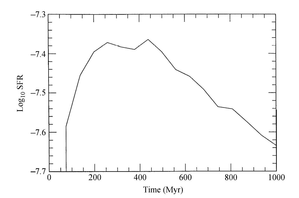
Fig. 6.17 A model of the total star formation rate (in units of \(M_\odot/{\rm pc^2/yr}\)) for the disk of the Milky Way as a function of time. Image Credit: Carroll & Ostlie (2007); Figure adapted from Burkert, Truran, & Hensler (1992).#
To understand the birthrates of stars and their contribution to the chemical evolution of the ISM, we must make some assumptions about the SFR Some astronomers assumed that the SFR is time-independent, while others argue for an exponentially decreasing function with time, or perhaps one that is proportional to some power of the surface mass density of the Galactic disk. One computer simulation (Burkert, Truran, & Hensler (1992)) produced an SFR that reached a maximum value and then decreased with time as the available gas and dust in the ISM was consumed. Other studies have considered the possibility that the SFR could be highly variable in both space and time, where such a situation could occur because of short timescale starburst activity.
The IMF is often bolded as a power-law fit of the form
where \(x\) can take on different values for various mass ranges and \(C\) is a normalization constant.
The first attempt to derive an IMF for the solar neighborhood was performed by Edwin E. Salpeter in 1955, where he argued for \(x = 1.35\). According to other determinations, it appears that \(x=1.8\) may be a better fit for \(7-35\ M_\odot\) stars (and perhaps as low as \(2\ M_\odot\)). For stars more massive than about \(40\ M_\odot\), \(x=4\) may be required, which implies that the production of massive stars drops off very rapidly with increasing mass.
Note
Most recently, Chabrier (2003) has argued for an IMF consisting of a log-normal distribution rather than a simple power-law.
For lower-mass stars, \(x\) is very difficult to determine through observational studies. The complications arise because the IMF must be decoupled with the present-day mass function and the SFR, which can be quite complicated itself.
6.2.2.1. The G-Dwarf Problem#
Attempts to use the SFR and the IMF to model the chemical evolution of the Galactic disk in the solar neighborhood have resulted in predictions that do not always agree with observations. If we assume that the first generation of stars were born without any metals (i.e., \(Z_o = 0\) or Pop III) and the chemical evolution of the ISM occurs within a closed box (i.e., no gas or dust is allowed to enter or leave the system), then the calculations predict too many stars of low metallicity when compared with observations. For instance this simple model suggests that roughly 1/2 of the stars in the solar neighborhood have \(Z<0.25 Z_\odot\) (\(Z_\odot \simeq 0.02\)). However, only about \(2\%\) of the F and G main sequence stars have such low \(Z\) values, where this is known as the G-dwarf problem.
One possible solution to the G-dwarf problem is to assume that the disk of our Galaxy formed with \(Z_o \neq 0\) and is known as prompt initial enhancement. This could occur if heavy-element enrichment of the ISM resulted from rapidly evolving massive stars before the gas and dust settled into the disk.
A second suggestion is that the disk accumulated mass over a significant period of time, where the closed-box assumption is invalid. In this scenario, a substantial infall of metal-poor material onto the Galactic disk occurred since it initial formation. Since a lower initial mass density would imply fewer stars formed during the early history of the disk, fewer metal-poor stars would be observed today.
Another proposal argues that the IMF was different int eh early history of the Galaxy, and a larger fraction of more massive stars were formed with correspondingly fewer low-mass stars. Since massive stars are short-lived, this hypothesis would result in fewer metal-poor stars today.
6.2.3. A Dissipative Collapse Model#
Another issue that must be addressed by a comprehensive theory of galactic evolution is the question of a free-fall collapse versus a slow, dissipative one.
A free-fall collapse is governed by the free-fall timescale (i.e., the dynamical timescale).
A dissipative collapse can be described in terms of the necessary time for the nebula to cool significantly (i.e., the cooling timescale).
If the cooling timescale \(t_{\rm cool}\) is much less than the free-fall timescale, then the cloud will not be pressure-supported and the collapse will be rapid (i.e., essentially in free-fall). However, if the cooling time exceeds the free-fall timescale, the gas cannot radiate its energy away fast enough to allow for a rapid collapse, and the gravitational potential energy that is released during the collapse will heat the nebula adiabatically.
To estimate the cooling timescale, we must first determine the characteristic amount of thermal kinetic energy contained within each particle in the gas. According to the virial theorem, if we assume that the gas is in quasistatic equilibrium, the average thermal kinetic energy of the gas must be related to its potential energy by \(-2\langle K \rangle = \langle U \rangle.\)
If we further assume that the gas has a mean molecular weight of \(\mu\) and contains \(N\) particles then the virial theorem gives
where \(m= \mu m_{\rm H}\) is the average mass of a single particle, \(R\) is the radius of the nebula, and \(M = Nm\) is the nebula’s total mass. In the last expression, we used a gravitationally bound, spherical mass distribution of constant density to estimate the potential energy of the system. Solving for the velocity dispersion \(\sigma = \langle v^2 \rangle^{1/2}\) gives
We may determine a characteristic gas temperature (i.e., the virial temperature) by equation the typical kinetic energy of a gas particle to its thermal energy, or
To estimate the cooling time we must determine the rate at which energy an be radiated away from the gas. This is done by expressing the cooling rate per unit volume as
where \(r_{\rm cool}\) has units of energy per unit time per unit volume, \(n\) is the number density of particles in the gas, and \(\Lambda(T)\) is a quantum mechanical cooling function. This cooling function \(\Lambda(T)\) includes the same physical process of bound-bound, bound-free, free-free, and electron scattering (see General Sources of Opacity in the Modern Astrophysics notes).
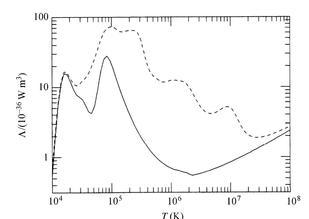
Fig. 6.18 The cooling function \(\Lambda(T)\). The solid line corresponds to a gas mixture of \(90\%\) hydrogen and \(10\%\) helium. The dashed line is for solar abundances. Image Credit: Carroll & Ostlie (2007); Figure adapted from Binney & Tremaine (1987).#
The two “bumps” in the cooling function (just above \(10^4\ \rm K\) and near \(10^5\ \rm K\)) correspond to the ionization/recombination temperatures of hydrogen and helium, respectively. Above about \(10^6\ \rm K\), the cooling is due to thermal bremsstrahlung and Compton scattering. The \(n^2\) dependence in the expression for \(r_{\rm cool}\) is explained in terms of the interactions between pairs of particles in the gas (i.e., collisions excite ions, atoms, or molecules that radiate the energy away in the form of photons and cool the gas).
If all the energy in the cloud is radiated away in a time \(t_{\rm cool}\), then
where \(V\) is the volume of the cloud and \(n\ (= N/V)\) is the number density of particles.
Exercise 6.3
Assume (for simplicity) that the proto-Galactic nebula in Exercise 6.2 was initially composed of \(90\%\) hydrogen and \(10\%\) helium. If we assume complete ionization, then the mean molecular weight is given by \(\mu \simeq 0.6\). The initial velocity dispersion of the particle in the gas is approximately \(\sigma = 160\ \rm km/s\).
What is the cooling time of the gas?
The cooling time given in Equation (6.8) depends on the number density \(n\) and the virial temperature \(T_{\rm virial}\). The virial temperature can be calculated directly using Equation (6.7) as
At this temperature our assumption that the gas was completely ionized is certainly valid. The number density of particle sin the gas is given by
This value should be compared to the typical number densities found in the Galactic molecular clouds today, which are \(n \sim 10^8-10^9\ {\rm m^{-3}}\).
Using \(\Lambda \sim 10^{-36}\ {\rm W\ m^3}\), the cooling time for the cloud is
Clearly, in this case \(t_{\rm cool} \ll t_{\rm ff} = 200\ {\rm Myr}\). Apparently the proto-Galactic nebula was capable of radiating energy away at a rate sufficient to allow for a free-fall collapse.
from scipy.constants import k, m_p

sec2yr = 3600*24.*356.25

sigma = 160e3 #velocity dispersion in m/s
T_virial = 0.6*m_p/(3*k)*sigma**2
print("The virial temperature of the proto-Galactic cloud is %1.1e K." % T_virial)
print("----------------------")
rho_o = 6.5e-23 #number density determined in Exercise 6.2
n = rho_o/(0.6*m_p)
print("The number density of particles in the gas cloud is %1.1e m^-3." % n)
print("----------------------")
cooling_func = 1e-36 #value of the cooling function for hydrogen
t_cool = 1.5*k*T_virial/(n*cooling_func)
print("The cooling time of the gas cloud is %1.3e s or %1.1f Myr." % (t_cool,t_cool/sec2yr/1e6))
The virial temperature of the proto-Galactic cloud is 6.2e+05 K.
----------------------
The number density of particles in the gas cloud is 6.5e+04 m^-3.
----------------------
The cooling time of the gas cloud is 1.983e+14 s or 6.4 Myr.
Consider the situation where \(t_{\rm cool} > t_{\rm ff}\). In this case the nebula is unable to efficiently radiate away the gravitational energy that is released by the collapse. As a result, the cloud’s temperature would rise adiabatically (i.e., heat does not enter/leave the system) as the cloud shrinks, resulting in an increasing internal pressure and a halt to the collapse.
After the collapse has halted the virial theorem governs the equilibrium conditions of the cloud. For the approximate values of \(T \sim 10^6\ \rm K\) and \(n \sim 5\times 10^4\ {\rm m^{-3}}\) characteristic of a proto-galactic cloud at time of formation of the first galaxies, the upper limit on the mass that can cool and collapse is \({\sim}10^{12}\ M_\odot\), with a corresponding radius of about \(60\ \rm kpc\).
In regions of the cloud where the gas temperature decreased to a level of hydrogen recombination \((T{\sim}10^4\ {\rm K})\) the mass limit becomes \({\sim}10^8\ M_\odot\). Thus, the galaxies that are observed today would be expected to have masses in the range of \(10^8-10^{12}\ M_\odot\). The lower limit corresponds fairly well with the values of the smallest dwarf elliptical galaxies, and the upper limit agrees well with values measured for the most massive giant spiral galaxies (Sa-Sc). Although some giant ellipticals and cD galaxies exceed \(10^{12}\ M_\odot\), they have certainly been affected significantly by mergers throughout their histories and are not in virial equilibrium near their outer edges.
Although the proto-Galactic cloud was able to radiate away the initial release of gravitational energy content from the system, shortly after the collapse began a new source of energy became available. The deaths of the first generations of very massive stars meant that supernova shells struck the gas, and the gas was reheated to temperatures of \({\sim}10^6\ {\rm K}\), slowing the rate of collapse. However, calculations of the supernova production rate that are based on estimates of the IMF suggest that even this new source of energy was unable to slow the collapse appreciably.
6.2.4. The Hierarchical Merger Model#
The ELS model explains the emergence of populations of stars, but it clearly lacks in many other subtle areas. We need a model that can explain the
apparent age and metallicity differences among the globular clusters.
existence of distinct components of varying ages within the disk of our Galaxy (i.e., thick and thin disk).
A bottom-up approach that undergoes an hierarchical process of mergers appears to solved some of these problems with the ELS model. We should not build a dichotomy between top-down and bottom-up processes, where it is likely that both contribute within a general model of galaxy formation. Within the 1970s and 1980s, astronomers realized that mergers play an important role in galactic evolution, where the hierarchical merger scenario received a great deal of attention because of new developments (observational and theoretical) regarding the nature of the early universe.
Most notably, density fluctuation existed in the overall distribution of matter shortly after the birth of the universe (via the Big Bang). Our current understanding of those fluctuations suggest that the most common density perturbations occurred on the smallest mass scales. Density fluctuations involving \(10^6-10^8\ M_\odot\) were much more common than those for \(\geq 10^{12}\ M_\odot\).
Consider the formation of the Milky Way as an example of the hierarchical merger process. As \(10^6-10^8\ M_\odot\) proto-Galactic fragments were gravitationally attracted to one another, they began to merge into a growing spheroidal mass distribution.
Initially, many of the fragments evolved in virtual isolation, forming stars and globular clusters in their centers. As a result, they developed their own chemical histories and unique abundance signatures.
In the inner regions of the growing spheroid (where the density of matter was greater), its rate of collapse and subsequent evolution would have been more rapid. This resulted in the production of the oldest stars that are observed today, together with a greater degree of chemical enrichment (e.g., old, metal-rich central bulge).
In the rarefied outer regions of the Galaxy, chemical evolution and star formation would have been much slower.
According to the hierarchical model, collisions and tidal interactions between merging fragments disrupted the majority of the fragments and left exposed some of the globular cluster cores. The disrupted systems would have led to the present distribution of the field halo stars, while leaving the remaining globular clusters scattered throughout the spheroid. Those proto-Galactic fragments that were initially moving in a retrograde direction (relative to the eventual orbital motion of the Galactic disk and inner halo) produced the net zero rotation of the outer halo that is observed today.
The rate of collisions would have been greater near the center of the Galaxy, disrupting some proto-Galactic fragments first and building the bulge more rapidly than the halo. According to this picture, the spheroidal component of the Galaxy can be considered as forming from the inside out.
The globular clusters still present in the Galaxy today probably represent only some \(10\%\) of the initial number that formed from proto-Galactic fragments. THe other \(90\%\) were disrupted by collisions and tidal interactions during the early merger process and by subsequent ongoing effects of dynamical friction. This may help to explain the relative uniformity in the masses of globular clusters observe today, which is \({\sim}10^5-10^6\ M_\odot\).
Low-mass globular clusters have small gravitational binding energies, which allowed them to be disrupted comparatively easily and rapidly when the Galaxy was young. The dynamical friction is also strongly dependent ont the mass of the cluster \((f_d \propto M^2)\) so that massive clusters would have spiraled rapidly into the inner regions of the Galaxy, which allowed for stronger and more frequent interactions that ultimately disrupted them.
Because of the isolation of the outer reaches of the Galaxy and the slower rate of evolution there, the proto-Galactic fragments in that region would have evolved almost like individual dwarf galaxies for a time. The significant number of dSph galaxies still present in the Local Group are assumed to be surviving proto-Galactic fragments. There is clear evidence of ongoing mergers today (e.g., the dSph Sagittarius galaxy and the Magellanic Stream) indicating that the construction of the Milky Way’s halo is still a work in progress.
6.2.5. Formation of the Thick and Thin Disks#
Formation of the Thick Disk
As the gas clouds of disrupted proto-Galactic fragments collided, the collapse became largely dissipative. This means that the gas began to settle slowly toward the central region of the Galaxy. Because of the presence of some initial angular momentum in the system (introduced through torques from other neighboring proto-galactic clouds), the collapsing material eventually became rotationally supported and settled into a disk about the Galactic center. The already-formed halo stars did not participate in the collapse to the disk because their collisional cross-sections were now too small to allow them to interact appreciably, expect through gravitational forces.
One model of thick-disk formation suggests that the thick disk may have formed around the Galactic midplane with a characteristic temperature of \(T\sim 10^6\ \rm K\). By equating the kinetic energy of a typical particle in the gas to its gravitational potential energy above the disk midplane, the approximate scale height \(h\) of the gas disk can be estimated.
To determine the local acceleration of gravity \(g\) at a height \(h\) above the midplane, imagine that the disk has a mass density \(\rho\) given by
where \(\rho_o\) is the mass density in the Galactic midplane. According to the gravitational version of “Gauss’ law”,
where the integral is over a closed surface that bounds the mass \(M_{\rm in}\), and \(\mathbf{g}\) is the local acceleration of gravity at the position \(d\mathbf{A}\). If \(h\) is much smaller than the diameter of the disk, then we can use a Gaussian cylinder of height \(2h\) and cross-sectional area \(A\) that is centered on the midplane to evaluate the integral as
where \(M_{\rm in}\) is the amount of disk mass contained within the cylinder. The interior mass can be estimated by integrating the mass density throughout the volume of the cylinder, or
Upon substitution, we have the local acceleration of gravity at a height \(h\) as
The gravitational potential energy of a particle of mass \(m\) at a height $h above the midplane is given by
Equating the potential energy to the average thermal kinetic energy of a particle (\(K = (3/2)kT\)), we find that
Exercise 6.4
Assume that the gas in the proto-Galactic thick disk had a characteristic temperature of \(T\sim 10^6\ \rm K\) and that the central mass density was comparable to the value that is estimated today for the solar neighborhood, \(\rho_o \simeq 0.19\ M_\odot/{\rm pc^3}\).
What is the estimated scale height?
The scale height depends on the characteristic temperature \(T\) and the assume density \(\rho_o\). We must first convert the density into SI units because \(k\) does not have an easy galactic conversion. Converting \(\rho_o\) produces
Using the converted value for \(\rho_o\) we find
where we have used the mass of a hydrogen atom for \(m\). The measured value for the height of thick disk is \(\sim 1\ \rm kpc\).
from scipy.constants import parsec, G, k, m_p
import numpy as np

M_sun = 1.989e30 #mass of Sun in kg
rho_o = 0.19*M_sun/parsec**3
print("The central mass density of the solar neighborhood converted to SI units is %1.2e kg/m^3." % rho_o)
print("-----------------")

T_char = 1e6 #characteristic temperature in K
C = 4*(np.exp(1)-1)/np.exp(1) #factor from integral of 2e^(-z/h) from 0 to h
h_T = np.sqrt(3*k*T_char/(C*np.pi*G*m_p*rho_o))
print("The scale height h is %1.2e m or %1.2f kpc." % (h_T, h_T/parsec/1000))
The central mass density of the solar neighborhood converted to SI units is 1.29e-20 kg/m^3.
-----------------
The scale height h is 6.03e+19 m or 1.95 kpc.
In regions where the gas was more locally more dense, it cooled more rapidly, since \(t_{\rm cool} \propto 1/n\). This was accomplished first through thermal bremsstrahlung and Compton scattering. After the temperature reached \({\sim}10^4\ \rm K\) (via the radiation emitted) by hydrogen atoms, the H I clouds could form and begin producing stars.
Within a few million years, the most massive stars underwent core-collapse supernova detonations and their shocks began to reheat the gas between the molecular clouds, which maintained the temperature of the intercloud gas at roughly \(10^6\ \rm K\). At the same time, the production of iron in the supernovae raised the metallicity from an initial value of \([{\rm Fe/H}] < -5.4\) to \([{\rm Fe/H}] = -0.5\). About \(400\ \rm Myr\) after the first stars were created in the thick disk, star formation nearly ceased. In total, a few percent of the mass of the gas was converted into stars during this thick-disk producing period of the Galaxy’s evolution.
A modified version of the thick-disk formation model described above suggests that the infalling gas was initially much cooler. This meant that the gas (and dust) was able to settle onto the midplane with a much smaller scale height, similar to today’s think disk. Star formation was then able to proceed due to the greater local density of gas and dust. As a direct result of a significant merger event with a proto-Galactic fragment some \(10\ \rm Gyr\) ago, the disk was reheated by the energy of the interaction, which caused it to puff up to its present \(1\ \rm kpc\) scale height.
Formation of the Thin Disk
After the formation of the thick disk, cool molecular gas continued to settle onto the midplane with a scale height of approximately \(600\ \rm pc\). During the next several billion years, star formation occurred in the thin disk.
The process of maintaining the scale height was essentially a self-regulating one. Fi the disk became thinner, its mass density would increase. This would cause the SFR to increase, which produced more supernovae and reheated the disk’s intercloud gas component. The ensuing expansion of the disk would again decrease the SFR, which yielded fewer supernovae, and the disk would cool and shrink.
Despite the self-regulating process, the gas was depleted in the ISM and the SFR decreased from about \(0.04\ M_\odot/{\rm pc^3/Myr}\) to \(0.004\ M_\odot/{\rm pc^3/Myr}\). At the same time, the metallicity continued to rise, reaching \([{\rm Fe/H}] \approx 0.3\). The thickness of the disk decreased to \({\sim}350\ \rm pc\) because of the decrease in the SFR, which corresponds to the scale height of today’s thin disk. During the development of the think disk, some \(80\%\) of the available gas was consumed in the form of stars.
AS the remaining gas continued to cool, it settled into an inner, metal- and gas-rich component of the thin disk with a scale height of \(<100\ \rm pc\). Today most ongoing star formation occurs in the young, inner portion of the thin disk, corresponding to the component in which the Sun resides.
6.2.6. The Existence of Young Stars in the Central Bulge#
The existence of young stars in the central bulge of our Galaxy can be understood by arguing for recent mergers with gas-rich satellite galaxies. When those galaxies were disrupted by tidal interactions with the Milky Way, their gas settled into the disk and the center for the Galaxy, ultimately forming new stars. It also appears that the Milky Way’s central bar plays a role in the migration of dust and gas into the inner portion of the Galaxy by generating dynamical instabilities as it rotates.
6.2.7. The Formation of Elliptical Galaxies#
The nature of the Hubble sequence may ultimately correspond to
the mass of the individual galaxies,
the efficiency with which the galaxies made stars, and
the relative importance of free-fall collapse, dissipative collapse, and mergers.
As an example, it appears that many ellipticals may have formed the majority of their stars early in the galaxy building process, before the gas had a chance to settle into a disk. Late-type galaxies took a more leisurely pace.
Ellipticals probably formed from the collisions of already-existing spirals. The energy involved in the collision would destroy the disks of both galaxies and cause the merged system to relax to the characteristic \(r^{1/4}\) distribution of an elliptical.
Although \(N\)-body simulations have been successful to produce ellipticals from mergers with spirals, some questions remain.
The large number of globular clusters in ellipticals relative to spirals present a serious difficulty in arguing that cataclysmic collisions are the cause of all large elliptical galaxies.
Perhaps mergers can actually produce globular clusters by triggering star formation in clouds, in which case the larger specific frequency of globular clusters may not be a problem.
It is also possible that many of the observed globular clusters are captured dSph galaxies, just as \(\omega\) Cen appears to be in the Milky Way.
Elliptical galaxies are much more abundant relative to spirals in the centers of dense, rich clusters of galaxies, whereas spirals dominate in less dense clusters and near the periphery of rich clusters. This morphology-density relation was first reported in Dressler (1980). This effect may be partly explained by the increased likelihood of interactions in regions where galaxies are more tightly packed, destroying spirals and forming ellipticals.
A competing hypothesis is that ellipticals tend to develop preferentially near the bottoms of deep gravitational potential wells, even in the absence of interactions. Lower-mass density fluctuations in the early universe may have resulted in spiral galaxies, and the smallest fluctuations let to the formation of dwarf systems.
If this is the case, then the large number of dSph and elliptical galaxies that exist has a natural explanation in the much larger number of smaller fluctuations that formed in the early universe. This mechanism could help explain galactic morphology if the initial density fluctuations in the early universe were larges in what later became the centers of rich clusters. Because the gravitational potential well in those regions would have been deeper, the probability of collisions between proto-galactic clouds should have been correspondingly greater as well.
6.2.8. Galaxy Formation in the Early Universe#
Given the large number of fundamental problems that still remain in our development of a coherent theory of galaxy formation, it is fortunate that a meas exists (at least in principle) for testing our ideas by observing galactic evolution through time. Because of the finite speed of light, when astronomers look farther out into space, we are literally looking back in time.
Galaxies that are \(1\ \rm Mpc\) away emitted their light more than \(3\ \rm Myr\) ago.
This means that the light we observe today coming from the galaxy itself is more than \(3\ \rm Myr\) old and we are seeing the galaxies as they were in the past.
Butcher & Oemler (1978) noted that there appeared to be an overabundance of galaxies in two distant clusters. They speculated that there may have been a significant evolution in galaxies over time, which led to the types of objects we see closer to us today. The Butcher-Oemler effect suggests that galaxies in the early universe were bluer on average than they are today, which indicates an increased level of star formation.
The morphology-density relation has also been shown to be time-dependent. As observations probe earlier times, elliptical and lenticular galaxies become less abundant relative to spiral galaxies. This suggests an evolution from later Hubble types to earlier types over time. This is just what would be expected if some earlier Hubble-type galaxies form from the mergers of spirals.
In 2004, the Space Telescope Science Institute released the Hubble Ultra Deep Field (HUDF). THe HUDF image is a composite of two images taken by: (1) the Advanced Camera for Surveys (ACS) and (2) the Near-Infrared Camera and Multi-Object Spectrometer (NICMOS). The region of the sky contained in the HUDF image is only \(3^{\prime}\) on a side, centered on a point \((\alpha = 3h32m40s,\ \delta = -27^\circ 48^\prime 00^{\prime\prime})\) in the constellation of Fornax. The image required a total exposure time of \(11.3\) days for ACS and \(4.5\) days for NICMOS.

Fig. 6.19 This view of nearly 10,000 galaxies is called the Hubble Ultra Deep Field. The snapshot includes galaxies of various ages, sizes, shapes, and colors. Image Credit: NASA, ESA, and S. Beckwith (STScI) and the HUDF Team.#
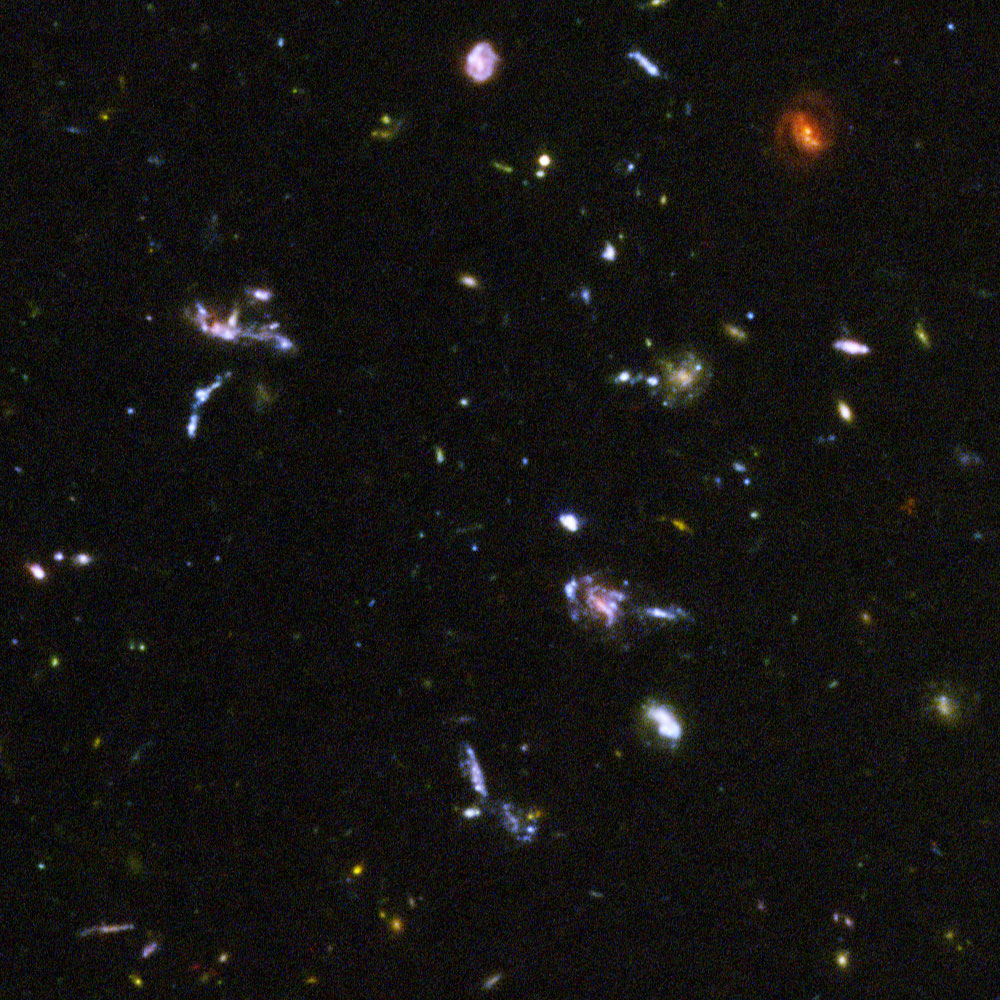
Fig. 6.20 Portion of the HUDF image highlighting a sample of the most distant galaxies. Image Credit: NASA, ESA, and S. Beckwith (STScI) and the HUDF Team.#

Fig. 6.21 This image taken by Webb’s Near-Infrared Camera (NIRCam) shows the galaxy cluster SMACS 0723 as it appeared 4.6 billion years ago, with many more galaxies in front of and behind the cluster. This field was also imaged by Webb’s Mid-Infrared Instrument (MIRI), which observes mid-infrared light. Image Credit: NASA, ESA, CSA, and STScI.#
The HUDF reveals some very distant galaxies as they existed \(400-800\ \rm Myr\) after the Big Bang. In the close-up portion of the HUDF, the very distant galaxies appear quite different from the relatively nearby majestic spirals and ellipticals that are seen in the present-day universe.
Observations like these suggest that the abundance of strange-looking, remote, blue galaxies seen in the early universe may be the building blocks of today’s Hubble sequence of galaxies. They probably represent the proto-galactic fragments responsible for the hierarchical mergers that are still occurring today at a much diminished rate.
6.3. Homework#
Problem 1
Use the age for the Milky Way’s oldest globular clusters and the orbital velocity of the LSR to estimate the greatest distance from which globular clusters could have spiraled into the nucleus due to dynamical friction. Compare your answer with the size of the Milky Way’s central bulge. Use \(5\times 10^6\ M_\odot\) for the cluster’s mass.
Problem 2
The Large Magellanic Cloud (which has a mass of about \(2\times 10^{10}\ M_\odot\)) orbits the Milky way at a distance of \(51\ \rm kpc\). Assuming that the Milky Way’s dark matter halo and flat rotation curve extend out to the LMC, estimate how much time it will tak for the LMC to spiral into the Milky Way (take \(C=23)\).
Problem 3
By equating the cooling timescale to the free-fall timescale, the maximum mass of a proto-galactic nebula is given by
Estimate the maximum mass of a proto-galactic nebula that can undergo a free-fall collapse if \(R = 60\ \rm kpc\). Assume that \(\Lambda \simeq 10^{-37}\ {\rm W\ m^3}\).
Problem 4
Estimate the scale height associated with a Galactic disk having a temperature of \(10^4\ \rm K\). With which component of our Galaxy might such a disk correspond today?
Bonus Problem
Use the python code below to reproduce the appearance of M51 and its companion, NGC 5195. Use 10 rings of 50 stars each and let the intruder galaxy have \(1/4\) the mass of the target galaxy. Use \((x,\ y,\ z) = (30,-30,0)\) for the initial position of the intruder galaxy, and use \((v_x,\ v_y,\ v_z) = (0, 0.34, 0.34)\) for its velocity. Follow the motion for \(648\ \rm Myr\) or 540 time steps.
(a) When does the calculated appearance of the target and host galaxies resemble the figure? Indicate the simulation times.
(b) What happens to the system near the end of this time period?
(c) Rerun the program, changing the initial \(x\) coordinate from \(30\rightarrow -30\) (and leaving everything else the same). Describe the difference in the outcomes.
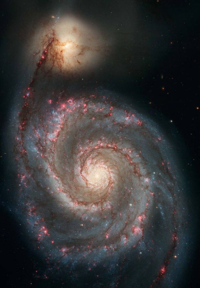
Fig. 6.22 The graceful, winding arms of the majestic spiral galaxy M51 appear like a grand spiral staircase sweeping through space. They are actually long lanes of stars and gas laced with dust. Such striking arms are a hallmark of so-called grand-design spiral galaxies. In M51, also known as the Whirlpool galaxy, these arms serve an important purpose: they are star-formation factories, compressing hydrogen gas and creating clusters of new stars. Image Credit: ASA, ESA, S. Beckwith (STScI) and the Hubble Heritage Team (STScI/AURA).#
!pip install rebound #install rebound first
import rebound
import matplotlib.pyplot as plt
import numpy as np
import os

host_galaxy_mass = 5*2e10 #host galaxy mass in M_sun
intruder_mass = host_galaxy_mass/4. #intruder galaxy mass in M_sun
delta_t = 1.2e6 #output interval
integ_time = 100*delta_t #number of time steps to run

pc2AU = 2.06265e5 #number of AU in 1 pc
dist_unit = 500*pc2AU
vel_unit = dist_unit/delta_t
theta_p = np.linspace(0,2*np.pi,50)
r_min = 2.6#dist_unit

x_intruder = 40*dist_unit #initial x-position intruder
y_intruder = 40*dist_unit #initial y-position intruder
vy_intruder = 0.5*vel_unit #initial v_y intruder
vz_intruder = 0.5*vel_unit #initial v_z intruder

nrings = 10 #number of rings
nstars = 5 #number of stars per ring

def run_sim():
    sim = rebound.Simulation()
    sim.integrator = 'whfast'
    sim.units = ('yr', 'AU', 'Msun')
    sim.dt = 0.01*delta_t
    sim.ri_whfast.corrector = 11

    sim.add(m=host_galaxy_mass)
    ps = sim.particles
    for i in range(0,nrings):
        r_p = (r_min + 2.6*i)*dist_unit
        v_p = np.sqrt(sim.G*host_galaxy_mass/r_p)
        for j in range(0,nstars):
            x_p, y_p =  ps[0].x + r_p*np.cos(theta_p[j]), ps[0].y + r_p*np.sin(theta_p[j])
            vx_p, vy_p = ps[0].vx - v_p*np.sin(theta_p[j]), ps[0].vy + v_p*np.cos(theta_p[j])
            sim.add(m=0,x=x_p,y=y_p,vx=vx_p,vy=vy_p)
    sim.add(m=intruder_mass,x=x_intruder,y=x_intruder,vy=vy_intruder,vz=vz_intruder)
    sim.automateSimulationArchive("archive.bin",step=100,deletefile=True)

    sim.integrate(integ_time)
    return

def plot_frame(idx):
    sim = sa[idx]
    sim.move_to_hel()
    ps = sim.particles

    fig = plt.figure(figsize=(8,8),dpi=150)
    ax = fig.add_subplot(111)
    ax.plot(ps[0].x/dist_unit,ps[0].y/dist_unit,'k.', ms=20)
    for i in range(1,len(ps)):
        if ps[i].m==0:
            ax.plot(ps[i].x/dist_unit,ps[i].y/dist_unit,'b.',ms=5)
        else:
            ax.plot(ps[i].x/dist_unit,ps[i].y/dist_unit,'r.',ms=10)

    ax.set_ylim(-60,60)
    ax.set_xlim(-60,60)
    fname = "plots/frame%03i.png" % idx
    fig.savefig(fname,bbox_inches='tight',dpi=150)
    plt.close()

run_sim() #run simulation
#---------------------
sa = rebound.SimulationArchive("archive.bin")
#plot individual frames at each time step
if os.path.exists("plots"):
    fig_list = [f for f in os.listdir("plots")]
    for f in fig_list:
        os.remove("plots/%s" % f)
else:
    os.makdirs("plots")

for idx in range(0,len(sa)):
    plot_frame(idx)