The Structure of the Universe
Contents
7. The Structure of the Universe#
7.1. The Extragalactic Distance Scale#
7.1.1. Unveiling the 3rd Dimension#
In 1761, the method of trigonometric parallax was used to measure the distance to Venus, thereby calibrating the size of Kepler’s Solar System. Friedrich Wilhelm Bessel measured the subtle annual shift in the position of 61 Cygni (in 1862), where he combined the parallax method with his knowledge with the measured size of Earth’s orbit to discover that 61 Cyg is \({\sim}650,000\ \rm AU\) away (or \({\sim}10\ \rm ly\); \(1\ {\rm ly} = 63,241\ {\rm AU}\)).
Today, the surveyor’s method of trigonometric parallax can reach out past the Galactic center, or to \({\sim}9.2\ \rm kpc\) with the Gaia telescope. Another method of distance determination was with the moving cluster method that made it possible to determine the distance to the Hyades cluster. The technique of main-sequence fitting (or spectroscopic parallax) can be used to find the distances to open clusters out to about \(7\ \rm kpc\) by comparing their main sequences on an H-R diagram with that of the Hyades cluster. The repeated application of a variety of methods using this pattern of calibration and measurement constitutes the steps of the extragalactic distance scale, or the cosmological distance ladder.
7.1.2. The Wilson-Bappu Effect#
Spectroscopic parallax can (in principle) provide reliable distances to remote stars out to \({\sim}7\ \rm Mpc\) away, although in practice it is employed with in a few \(100\ \rm kpc\) and is far enough to reach the Magellanic Clouds. Some stars have specific feature in their spectra that allow their absolute magnitudes (and hence their distances) to be calculated.
For example, the K absorption line of \(\rm Ca\) can be quite broad, reaching maximum strength at spectral type \(\rm K0\). In late-type stars with chromospheres (e.g., \(G,\ K,\ \text{and } M\) spectral types), a narrow emission line is seen, centered on the wide K absorption line. The width of this emission line is strongly correlated with a star’s absolute visual magnitude, valid over a range of \(15\) magnitudes, and called the Wilson-Bappu effect (Wilson & Vainu Bappu (1957)).
7.1.3. The Cepheid Distance Scale#
For more distant objects, astronomers turn to the period-luminosity relation for Cepheids. Before this relation could be used, it had to be calibrated by finding a classical Cepheid. The nearest one (Polaris) was too far away (\({\sim}200\ \rm pc\)) for trigonometric parallax to be useful when the first calibrations were being performed in the early 20th century.
In 1913, Ejnar Hertzsprung used the Sun’s motion of \(16.5\ \rm km/s\) with respect to the LSR to provide a longer baseline for parallax measurements. It was this technique of secular parallax that enabled him to determine the average distance to a classical Cepheid with a period of \(6.6\ \rm days\). Hertzsprung then used this information to calibrate the period-luminosity relation, where Shapley carried out a similar procedure. The distances to more Cepheids have been measured by parallax and other methods since then, and the period-luminosity relation has become well established. Astronomer today use a period-luminosity relation in the form (Marengo et al. (2010))
where \(\beta\) accounts for the finite width of the instability strip on the H-R diagram. Carroll & Ostlie (2007) use \(\alpha = -3.53\) and \(\beta = 2.13(B-V) - 5.66\), where Marengo et al. (2010) use \(\alpha = -3.37 \pm 0.06\) and \(\beta = -5.65 \pm 0.02\) in the K band. In both cases, \(P\) is the pulsation period in units of days, where \(B-V\) refers to the color index. For classical Cepheids \(B-V\approx 0.4\text{ to } 1.1\). After the star’s absolute magnitude has been calculated, it can be combined with the star’s apparent magnitude to give its distance modulus.
Cepheid variable stars immediately proved their worth as stellar yardsticks. It was in 1917 that Shapley measured the distances to Pop II Cepheids in globular clusters, thereby determining his estimates for the diameter of the Galaxy and the distance of the Sun from its center. In 1923, Edwin Hubble discovered several Cepheid in M31 and announced that it was \(285\ \rm kpc\) away. It was Hubble’s series of observations that established M31 as an external galaxy, not a smaller nebula within the borders of the Milky Way.
The existence of a correlation between a Cepheid’s pulsation period and it absolute magnitude meant that these stars could be used as standard candles to determine distances many years before the physical processes that cause the pulsations were understood.
At the time, it was not known that 3 types of pulsating stars were used to determine the size of the Galaxy and the distance to M31. Although the existence of interstellar dust clouds had been established, the existence of diffuse interstellar dust and gas capable of extinguishing starlight had not yet been demonstrated. Leavitt’s variables in the Magellanic Clouds were classical Cepheids (Pop I stars), while those observed in the globular clusters by Shapely were W Virginis and RR Lyrae stars (both Pop II).
The W Viriginis stars are about \(1.5\ \text{mag}\) fainter than classical Cepheids of the same period, which corresponds to a lower luminosity by a factor of 4. After Hertzsprung and (later) Shapley calibrated the period-luminosity relation, they used nearby classical Cepheids but neglected the effect of extinction. Neither realized that dust in the Galactic disk dimmed these stars by (coincidentally) about \(1.5\ \text{mag}\).
By chance the resulting period-luminosity relation was just about right when used with W Virginis stars. However, it would give an underluminous result with classical Cepheids. When Hubble used this calibration to determine the distance to M31, the apparent magnitudes of his Cepheids were correct but his estimates of the absolute magnitudes were too large. Consequently, their distance module \((m-M)\) and the distances themselves were underestimated. The stars were thought to be dimmer and closer rather than brighter and farther away, and so their parent galaxies were measured at roughly 1/2 of their actual distances and half their actual sizes.
Shapley fared no better with his observations of the (unknown to him) W Virginis stars in the globular clusters. Although he unwittingly used the right variety of star for the calibration of the period-luminosity relation. Extinction due to dust within the Galactic disk dimmed the starlight and increased the stars’ apparent magnitudes. Because the importance of extinction was not yet recognized, Shapely incorrectly attributed his stars’ faintness to their remoteness. As a result, his distances to the globular clusters were too great, as was the size he calculated for the Galaxy.
Something was obviously wrong. It appeared that the Milky Way was much larger than any of the galaxies surveyed. Trumpler (1930) showed that interstellar extinction could remedy part of the problem. The rest of the puzzle was solved by Baade (1956), who showed that there are two types of Cepheids: (1) the classical Cepheids and (2) the intrinsically fainter W Virginis stars. With these corrections, the measured distances and sizes of the other galaxies doubled and the Milky Way was reduced to a size that was a bit smaller than M31.
In the early 1990s, the calibration of the period-luminosity relation was carried out using data obtained by the Hipparcos mission. Hipparcos astronomers measured the parallax angles of 273 Cepheids and used the resulting distances to derive the period-luminosity relation. This was the first period-luminosity relation obtained from a direct distance measurement, and it is interesting that the result was nearly identical to an expression obtained by Sandage & Tammann (1968). Although further adjustments are sure to follow Cepheids certainly provide a firm foundation measuring the distances to other galaxies.
Interstellar extinction is still the largest source of error when Cepheids are used as standard candles, and there may also be a weak dependence on metallicity. The extinction problem can be reduced by observing these stars at IR wavelengths, since IR light more readily penetrates dusty regions. Because Cepheids are about \(3\times\) dimmer in the IR, astronomers have not stopped searching for them at visible wavelengths.
7.1.4. Supernovae as Distance Indicators#
Supernovae can be used in several ways to measure extragalactic distances. Suppose the angular extent \(\theta(t)\) of a supernova’s photosphere is observed. The angular velocity of the expanding gases \(\omega\ (=\Delta \theta/\Delta t)\) can be found by comparing two observations separated by a time \(\Delta t\). If \(d\) is the distance to the supernova, then the transverse velocity of the expanding photosphere is \(v_\theta = \omega d\).
Assuming that the expansion is spherically symmetric, the transverse velocity should be equal to the ejecta’s radial velocity \(v_{\rm ej}\) obtained from the supernova’s Doppler-shifted spectral lines. Then the distance to the supernova is \(d= v_{\rm ej}/\omega\).
Most supernovae are too distant for the above method to be employed, where another strategy is adopted. It assumes that the expanding shell of hot gases radiates as a blackbody. Then the supernova’s luminosity is given by the Stefan-Boltzmann law,
where \(R(t)\) is the radius of the expanding photosphere and \(t\) is the age of the supernova. If we assume that the ejecta’s radial velocity has remained nearly constant, then \(R(t) = v_{\rm ej}t\). The effective temperature \(T_e\) of the photosphere comes from the characteristics of its blackbody spectrum. Once the luminosity is found, it can be converted to an absolute magnitude and then used to find the distance to the supernova by comparing it with the apparent magnitude.
The photosphere of the expanding shell of a supernova is neither perfectly spherical nor a perfect blackbody. Difficulties with accurate values for interstellar extinction plague both methods, but the problem is more acute for core-collapse supernovae (Types Ib, Ic, and II), which are found near sites of recent star formation. Typical uncertainties in the distances obtained range from \(15-25\%\) for M101 to the Virgo cluster of galaxies, respectively.
Exercise 7.1
Twenty-five days after maximum light, the spectrum of an “average” Type Ia supernova is that of a black body with an effective temperature of \(6000 \pm 1000\ \rm K\). The speed of the shell’s photosphere (obtained from its Doppler shifted absorption lines) is \(9500 \pm 500\ \rm km/s\). The rise time to maximum light is \(17 \pm 3\) days.
When the average Type Ia supernova is \(42\ {\rm days}\) old, what is its luminosity and absolute magnitude?
To determine the luminosity of the supernova, we can use the Stefan-Boltzmann law. The radius of the shell can be estimated by the velocity of the shell’s photosphere and the age of the supernova. The luminosity is given as
The absolute magnitude of the supernova can be determined by comparing its luminosity to the Sun by
from scipy.constants import sigma
import numpy as np

day2sec = 3600*24
L_sun = 3.828e26 #solar luminosity in W
absM_Sun = 4.83 #absolute magnitude of the Sun in the visual

v_ej = 9500e3 #speed of ejecta in m/s
t_rise = 42*day2sec #rise time in seconds
T_e = 6000 #effective temperature in K
L = 4*np.pi*sigma*(v_ej*t_rise)**2*T_e**4
print("The luminosity of the Type Ia supernova after 42 days is %1.1e W." % L)
print("--------------")

M = absM_Sun - 2.5*np.log10(L/L_sun)
print("The absolute magnitude of the Type Ia supernova is approximatley %1.2f." % M)
The luminosity of the Type Ia supernova after 42 days is 1.1e+36 W.
--------------
The absolute magnitude of the Type Ia supernova is approximatley -18.81.
7.1.5. Type Ia Light Curves#
The most important way of using supernovae to measure distance takes advantage of the similarity of Type Ia light curves. These supernovae have blue and visual absolute magnitudes of \(\langle M_B \rangle \simeq \langle M_V \rangle \simeq -19.3 \pm 0.03\) at maximum light. If the peak magnitude of a Type Ia can be determined, its distance can also be determined.
Fortunately there is a well-defined inverse correlation between a Type Ia’s maximum brightness and the rate of decline of its light curve, and astronomers learned to use this information to more precisely determine the supernova’s intrinsic peak luminosity.
In practice, a supernova is observed over time at several wavelengths. The multicolor light curve shapes (MCLS) method (Riess, Press, & Kirshner (1996)), then compares the shape of the light curve to a family of parameterized template curves that allows the absolute magnitude of the supernova at maximum brightness to be determined (even if the supernova was not caught at its peak brilliance). The MLCS method also allows the reddening and dimming effect of interstellar dust to be detected and removed.
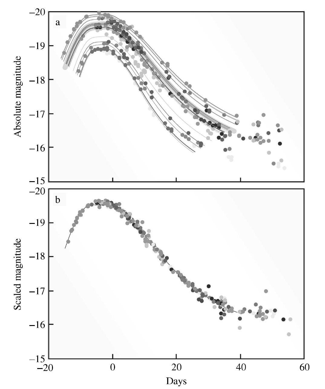
Fig. 7.1 Low-redshift Type Ia template light curves. (a) The light curves of several Type Ia supernovae, as measured. (b) The light curves after applying the time scale stretch factor. The vertical axis is the blue magnitude. Image Credit: Carroll & Ostlie (2007). Figure adapted from Perlmutter (2003)#
Another approach is the stretch method (Goldhaber et al. (2001)), which fits the B and V magnitude light curves with a single template light curve that has been stretched (or compressed) in time. The peak magnitude is then determined by the stretch factor. These techniques allow astronomers to use Type Ia supernovae to determine distance with an uncertainty approaching just \(5\%\), which corresponds to an uncertainty in the distance modulus \(m-M\) of \(0.1\ \rm {mag}\).
Exercise 7.2
The Type Ia supernova SN 1963p in the galaxy NGC 1084 had an apparent blue magnitude of \(B = 14.0\) at peak brilliance.
With an extinction of \(0.49\ \rm mag\) to that galaxy, what is an approximate distance to the supernova?
The distance modulus formula with extinction can be used to estimate the distance to Type I supernovae due to their characteristic absolute \(B\) magnitude of \(M_{B} = -19.3\). Substituting the apparent \(B\) magnitude, we find
m_B = 14
A_B = 0.49
M_Ia = -19.3

exp = (m_B-M_Ia-A_B+5.)/5.
d = 10**exp
print("The distance to the supernova is approx. %2.1f Mpc." % (d/1e6))
The distance to the supernova is approx. 36.5 Mpc.
Because Type Ia supernovae are about \(13.3\) magnitudes brighter than the brightest Cepheid variable (\(-19.3\) vs. \(-6\)), this method is capable of reaching out more than \(500\times\) farther than with Cepheids, providing estimates of truly cosmological distances \(>1000\ \rm Mpc\). Sophisticated supernova search programs are carried out that more than compensate for the unlikely probability of detecting an explosion in a specific galaxy by scanning large numbers of galaxies in a wide field of view.
Near the end of the 20th century, two teams of astronomers made careful observations of high redshift Type Ia supernovae and discovered that the expansion of the universe is accelerating. The Nancy Grace Roman Space Telescope (aka SuperNova Acceleration Probe aka Joint Dark Energy Mission) will search for extrasolar planets using microlensing, probe the probe the chronology of the universe, and answer basic questions about dark energy using observations of distant supernovae.
Note
Type II supernovae are dimmer than the Type Ia by about \(2\ \rm mag\) and can be seen only about \(40\%\) as far away (at best).
7.1.5.1. Using Novae in Distance Determinations#
From the sizes of their expanding photospheres, novae can be used in the same manner as supernovae to determine distances. Although there is a wide variation in the absolute magnitudes of novae at peak light, there is a relation between a nova’s maximum visual magnitude \(M_v^{\rm max}\) and the time it takes for its visible light to decline by two magnitudes. Consequently, novae can serve as standard candles.
The physical reason why this relationship holds for novae is that more massive, smaller white dwarfs produce greater compression and heating of the accreted gases on their surfaces. A runaway thermonuclear reaction may be initiated with a smaller accumulated mass. The less massive surface layers are more readily ejected, and the nova declines more rapidly. The average rate of decline over the first \(2\ \rm mag\) is written as \(\dot{m}\) (in \(\rm mag/day\)) and can be expressed as
for Galactic novae, with an uncertainty of about \(\pm 0.4\ \rm mag\) (Cohen (1985); see here for details). After fading two magnitudes, the brightest novae are about as luminous as the brightest Cepheids, which means that these two methods reach to about \(20\ \rm Mpc\) or just past the Virgo cluster.
Note
There are several variants for the rate of decline for novae, which use time to decline by a given magnitude (e.g., \(2\ \rm mag\), \(3\ \rm mag\), etc.). See Hachisu et al. (2020) and Chomiuk et al. (2021) for recent developments.
7.1.6. Secondary Distance Indicators#
Supernovae are unpredictable and somewhat rare occurrences for a given galaxy, where astronomer must use secondary methods to measure the distance to more remote galaxies. These secondary distance indicators require a galaxy with an established distance for their calibration.
One way of seeing farther involves using the brightest objects in a galaxy. For example, the three brightest giant H II regions in a galaxy can be used as a standard candle. These regions are visible at great distances, and may contain up to \(10^9\ M_\odot\) of ionized hydrogen.
Measurements of the angular sizes of the H II regions and the apparent magnitude of the galaxy can be compared with similar measurements for other galaxies with known distances. This makes it possible to calculate the H II regions’ linear sizes (in \(\rm pc\)), along with the galaxy’s absolute magnitude. However, since the diameter of an H II region is difficult to define unambiguously, this procedure is relatively insensitive to distance and must be used carefully.
The brightest red supergiants seem to have about the same absolute visual magnitude in all galaxies. Apparently, mass loss reduces the brightest red supergiants to the same maximum mass, which results in their having about the same luminosity. Sampling a number of galaxies revealed the average visual magnitude of the three brightest red stars to be \(M_V = -8.0\). Because individual stars must be resolved for this method, its range is the same as for spectroscopic parallax, or about \(7\ \rm Mpc\).
7.1.7. The Globular Cluster Luminosity Function#
The limited sampling inherent in the secondary methods (with “the three brightest …”) can lead to errors. It is statistically more secure to take a more complete inventory using some class of objects associated with a galaxy, and then describe how the objects vary with magnitude.
The globular cluster luminosity function \(\varphi(M_B)\) for the globular clusters around four giant elliptical galaxies in the Virgo cluster have been used. The function is given as \(\varphi(M_B)dM_B\) to represent the number of globular clusters with an absolute blue magnitude between \(M_B\) and \(M_B + dM_B\). The distribution is well-described by a Gaussian function with a well-defined peak at a turnover magnitude, which is \(M_o \simeq -6.5\) for elliptical galaxies in the Virgo cluster. The value of the turnover magnitude provides a standard candle that can be used to find the distance to the globular clusters surrounding another galaxy.
Note
Notice that the value of \(M_o\) depends on the distance to the Virgo cluster used in calculating the absolute magnitudes.
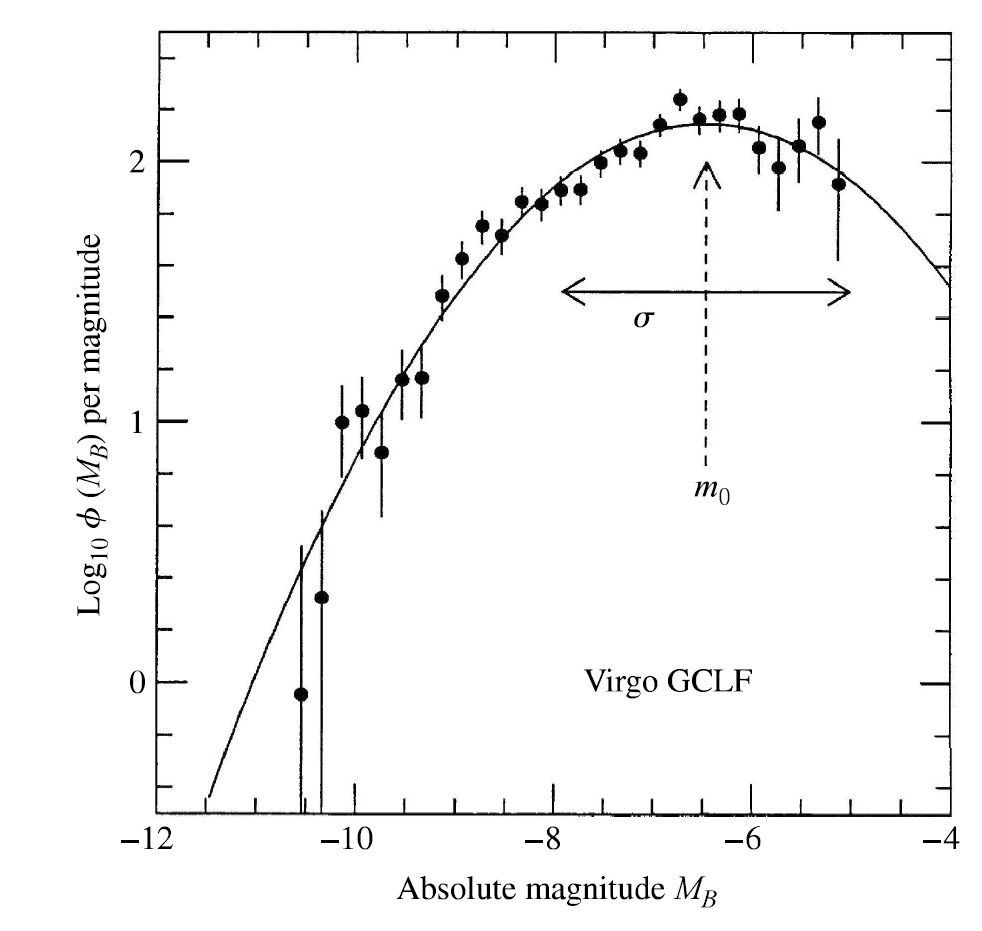
Fig. 7.2 The luminosity function for the globular clusters around four giant elliptical galaxies in the Virgo cluster. A distance of \(17\ \rm Mpc\) and \({\sim}2000\) clusters brighter than \(B=26.2\) were used. Image Credit: Carroll & Ostlie (2007). Figure adapted from Jacoby et al. (1992).#
The procedure to determine these distances is to measure the luminosity function for the galaxy in question and compare its apparent turnover luminosity \(m_o\) with \(M_o\) for the Virgo cluster. The best results are achieved with galaxies have large numbers of globular clusters (e.g., giant ellipticals). It is desirable that the calculated \(\varphi(m_B)\) extend well past the turnover point. Overall this method should yield a value fora galaxy’’s distance modulus that is uncertain by only \({\sim}0.4\ \rm mag\), which corresponds to a uncertainty in the distance of about \(20\%\). Globular clusters are visible from vast distances, which may reach out beyond the Virgo cluster to \(50\ \rm Mpc\).
Unfortunately, it is not certain whether there is a universal globular cluster luminosity function that applies to all types of galaxies, although for 9 galaxies (including M31 and the Milky Way), the average value is \(M_o = -6.6 \pm 0.26\). The physical basis for the apparent agreement is unclear, but it is reasonable to suppose that the subsequent evolution of the host galaxies may not have significantly affected the individual clusters.
7.1.8. The Planetary Nebula Luminosity Function#
A galaxy’s planetary nebulae are determined using a similar statistical analysis through the planetary nebula luminosity function (PNLF). Using the Leo I group of galaxies, their luminosity increases with measurement of the absolute magnitude at \(\lambda = 500.7\ \rm nm\).
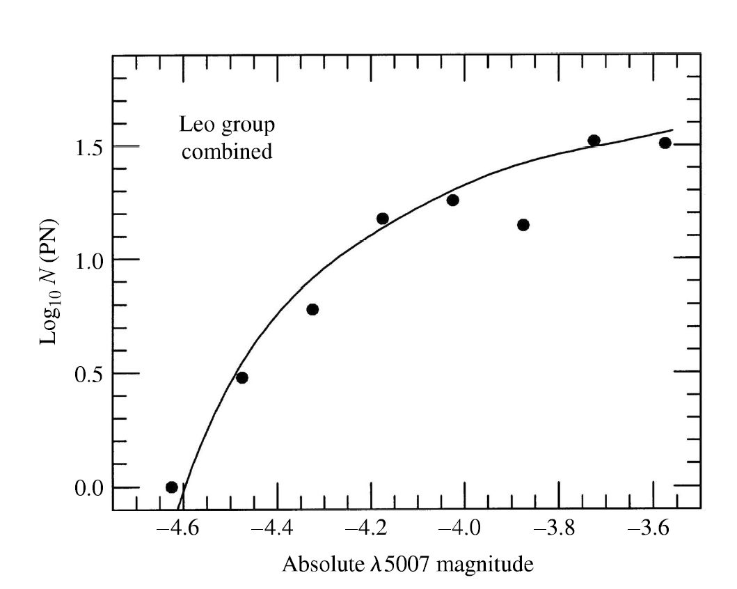
Fig. 7.3 The planetary nebula luminosity function for the Leo I group of galaxies. Image Credit: Carroll & Ostlie (2007). Figure adapted from Ciardullo et al. (1989).#
Using extragalactic planetary nebulae in this way is a reliable method of finding the distances to elliptical galaxies within about \(20\ \rm Mpc\). As a larger sample of galaxies was studied, the cutoff absolute magnitude is \(M_{5007} = -4.53\). This method can be adopted as a standard candle for the brightest planetary nebula. If the promise of this method is fulfilled, it should reach out to a distance of \(\sim 50\ \rm Mpc\).
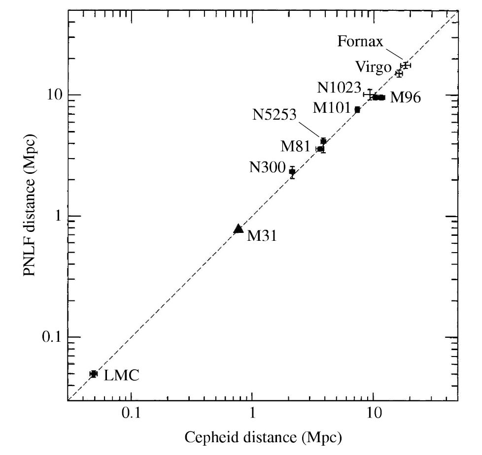
Fig. 7.4 A comparison between distances obtained using the planetary nebular luminosity function (PNLF) and Cepheids. Image Credit: Carroll & Ostlie (2007). Figure adapted from Jacoby et al. (1999).#
7.1.9. The Surface Brightness Fluctuation Method#
Astronomers turn to the global properties of galaxies to probe even farther (up to \(100\ \rm Mpc\) or more). One promising approach is to use how a CCD camera record the appearance of a galaxy. Some pixels will record more stars than others due to the spatial fluctuation in the galaxy’s surface brightness, but the overall appearance should become smoother with increasing distance. The results of a statistical analysis describe the magnitude of the pixel-to-pixel variation, and this is correlated with the galaxy’s distance. With HST, the surface brightness fluctuation method could reach out to \(125\ \rm Mpc\), but it is usually applied more locally.
7.1.10. The Tully-Fisher Relation#
The Tully-Fisher relation for spiral galaxies also provides a valuable tool for determining extragalactic distances. This is a relation between the luminosity of a spiral galaxy and its maximum rotation velocity.
Exercise 7.3
The rotation velocity \(W_R^i\) in M81 is approximately \(484\ \rm km/s\) and the apparent \(H\) magnitude is \(4.29\) (already corrected for extinction).
What is the infrared absolute magnitude \(M_H\) and distance to M81?
Using the relation Pierce and Tully (1992) (Eq. (4.6)), we can use the measured rotation velocity to find the \(H\) band absolute magnitude as:
With the apparent and absolute magnitudes in the \(H\) band, we can then calculate the distance to M81 using the distance modulus,
import numpy as np

W_R = 484 #measured rotation velocity of M81 in km/s
app_H = 4.29
abs_H = -9.5*(np.log10(W_R)-2.5) -21.67

print("The absolute H magnitude of M81 is %2.2f." % abs_H)
print("---------------------------")

d = 10**((app_H-abs_H+5)/5.)
print("The distance to M81 is %1.3e pc or %1.2f Mpc." % (d,d/1e6))
The absolute H magnitude of M81 is -23.43.
---------------------------
The distance to M81 is 3.493e+06 pc or 3.49 Mpc.
The appeal of the Tully-Fisher method of distance determination lies in its accuracy (typically \(\pm 0.4\ \rm mag\) in the IR) and its great range (as far as \(100\ \rm Mpc\)). Nearby spirals whose distances have been accurately measured by Cepheids can be used for its calibration.
The Tully-Fisher method has been applied to 161 spiral galaxies belonging to the Virgo cluster, which resulted in producing a 3D map of the cluster and that the Virgo cluster extends along the line-of-sight about \(4\times\) its diameter on the sky.
7.1.11. The \(D-\sigma\) Relation#
The analogous correlation for elliptical galaxies (the Faber-Jackson relation; \(L \propto \sigma_r^4\)) shows considerable scatter. The \(\mathbf{D-\sigma}\) relation compares the velocity dispersion \(\sigma\) to the diameter \(D\) of an elliptical galaxy. The galaxy’s angular diameter \(D\) out to a surface brightness level of \(20.75\ \rm {B{-}mag/arcsec^2}\).
Because the surface brightness is independent of galaxy’s distance (within \(500\ \rm Mpc\)), \(D\) is inversely proportional to the galaxy’s distance \(d\). If the galaxy were twice as far away, its angular diameter would be half as large. In this way, \(D\) provides a standard ruler rather than a standard candle. There is a tighter relationship between \(\sigma\) and \(D\) than there is between \(\sigma\) and \(L\). An empirical logarithmic relation between \(D\) and \(\sigma\) for the galaxies in a cluster (all at about the same distance) is
where the constant \(C\) depends on the distance to the cluster of galaxies. Unfortunately, there are no bright elliptical galaxies available for the accurate calibration of this \(D-\sigma\) method by primary distance indicators (e.g., Cepheids). However, because the slopes of the lines from a logarithmic plot of \(sigma\) vs. \(D\) are very nearly the same, the vertical distance between the lines for two different clusters is
Because \(D\) is inversely proportional to a galaxy’s distance \(d\), the relative distances between the two clusters can be found using
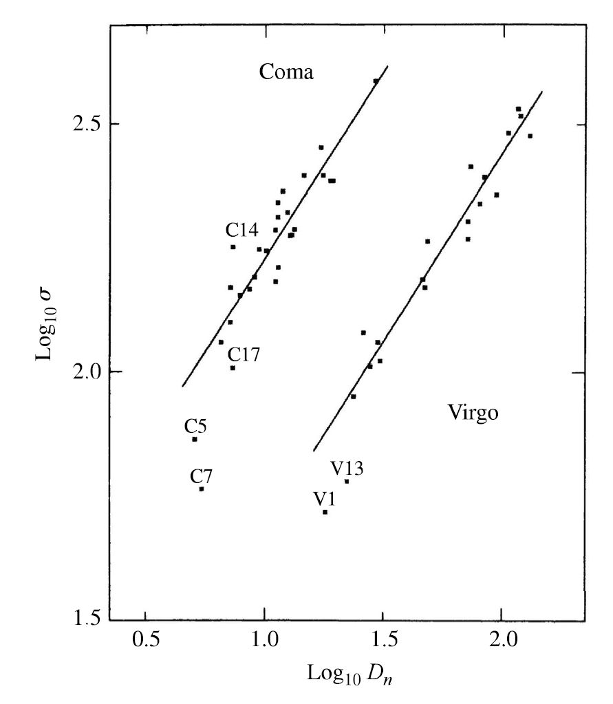
Fig. 7.5 A logarithmic plot of diameters \(D\) (in arcseconds) and velocity dispersion \(\sigma\) (in \(\rm km/s\)) for galaxies in the Virgo and Coma clusters. Image Credit: Carroll & Ostlie (2007). Figure adapted from Dressler et al. (1986).#
The \(D-\sigma\) relation can be a powerful tool for studying the distribution of galaxy clusters because the inherent brightness of giant elliptical galaxies. This technique also has the potential of exceeding the range of the Tully-Fisher relation.
Exercise 7.4
The \(y\)-intercept for a \(\sigma\) vs. \(D\) plot indicates that the value of \(C\) for the Virgo cluster is \(-1.237\), and for the Coma cluster it is \(-1.967\).
What is the ratio of distances between the two clusters of galaxies? How much farther is one galaxy cluster compared to the other?
The distance ratio between the two clusters can be determined through the ratio of distance formulae. This results in simply subtracting the values of \(C\) for the respective clusters and using the result as the exponent using a base-10, or
The distance ratio tells us that the Coma cluster is \(5.37\times\) farther away than the Virgo cluster.
C_Virgo = -1.237
C_Coma = -1.967

d_ratio = 10**(C_Virgo - C_Coma)
print("The relative distance between the two clusters is %1.2f." % d_ratio)
The relative distance between the two clusters is 5.37.
7.1.12. The Brightest Galaxies in Clusters#
Just as the brightest H II regions or the brightest red supergiants have been used to determine the distance to individual galaxies, the brightest galaxy in a cluster can be used to obtain the cluster’s distance.
From a composite luminosity function, we can see a sharp decline in the function at the bright end (more negative \(M\)), which indicates that the absolute magnitude of the brightest galaxy can be determined with some accuracy. The average value of the absolute visual magnitude for the brightest galaxy in ten nearby clusters is \(M_V = -22.83 \pm 0.61\), where this is \(3.2\) magnitudes brighter than a Type Ia supernova at peak brilliance and in principle, this method should reach \(4\times\) farther than with supernovae (to \(>4000\ \rm Mpc\)).
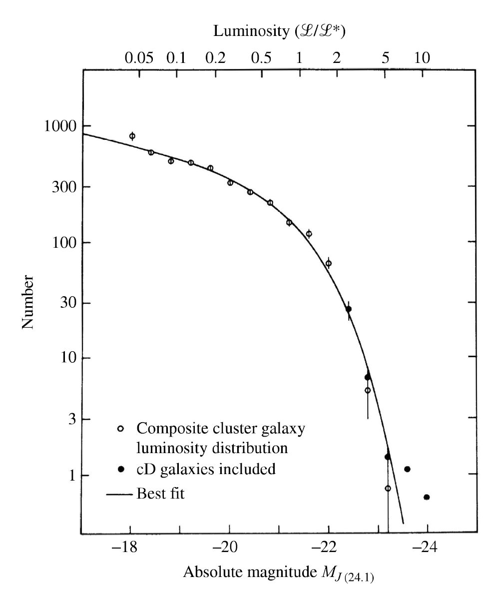
Fig. 7.6 A composite luminosity function for the galaxies in several clusters. Image Credit: Carroll & Ostlie (2007). Figure adapted from Schechter (1976).#
The danger in using this method is that galaxies and galaxy cluster both evolve. For example, the brightest galaxy in a contemporary cluster may not have existed in its present form billions of years ago. The giant cD galaxies often found at the centers of reich clusters are probably the result of galactic mergers. Using a general galaxy luminosity function calibrated with nearby clusters may not be appropriate for very distant, and consequently younger-looking clusters.
7.1.13. A Summary of Distance Indicators#
The extragalactic distance scale is not a simple ladder, with just on sequence of steps possible for measuring the greatest distances. Different astronomers use different techniques and choose different calibrations. There are variations with every method, and the relations are chosen only to representative.
Table 7.1 lists the distance to the Virgo cluster as determined by many of these methods. It also shows the uncertainty (in \(\rm mag\)) associated with each of these techniques. Overall, the distances are in good agreement, where the modern value is \(16.5 \pm 0.1\ \rm Mpc\) (see Mei et al. (2007)). These methods are sufficiently accurate to determine the features of our corner of the universe, out to a distance of a few \(100\ \rm Mpc\).
Method |
Uncertainty for |
Distance to |
Range |
|---|---|---|---|
Cepheids |
\(0.16\) |
\(15-25\) |
\(29\) |
Novae |
\(0.4\) |
\(21.1 \pm 3.9\) |
\(20\) |
Planetary nebula |
\(0.3\) |
\(15.4 \pm 1.1\) |
\(50\) |
Globular cluster |
\(0.4\) |
\(18.8 \pm 3.8\) |
\(50\) |
Surface brightness |
\(0.3\) |
\(15.9 \pm 0.9\) |
\(50\) |
Tully-Fisher relation |
\(0.4\) |
\(15.8 \pm 1.5\) |
\(>100\) |
\(D-\sigma\) relation |
\(0.5\) |
\(16.8 \pm 2.4\) |
\(>100\) |
Type Ia supernovae |
\(0.10\) |
\(19.4 \pm 5.0\) |
\(>1000\) |
7.2. The Expansion of the Universe#
In the early 1900s, astronomers began making systematic observations of the galactic radial velocities by measuring their Doppler-shifted spectral lines. It was hoped that if the motions of these objects were found to be random, then the Sun’s motion in the Milky Wya should be related to the vector sum of the radial velocities of the spiral nebulae.
It was Vesto Slipher who first discovered that this plan was doomed to failure. The velocities of the spiral nebulae were not random. Instead, most of the spectra showed redshifted spectral lines. Slipher announced in 1914 that most of the 12 galaxies he surveyed were rapidly moving away from Earth, although M31’s blueshifted spectrum indicated it was approaching Earth at nearly \(300\ \rm km/s\). It was quickly realized that these galaxies were not only moving away from Earth but moving away from each other as well.
Astronomers began to talk about these galactic motions in terms of an expansion. Meanwhile, Slipher continuted his measurements, and by 1925, he had examined \(40\) galaxies with spectra showing redshifted lines were much more common than those exhibiting blueshifts. Slipher concluded that nearly every galaxy he examined was rapidly receding from Earth.
7.2.1. Hubble’s Law of Universal Expansion#
In 1925, Hubble discovered Cepheid variable stars in M31, which established that the Andromeda “nebula” was in fact an external galaxy. Hubble continued his search for Cepheids, while determining the distances to \(18\) galaxies. He combined his results with Slipher’s velocities and discovered tha a galaxy’s recessional velocity \(v\) was proportional to its distance \(d\). In 1929, Hubble presented his results in a paper at a meeting of the National Academy of Sciences (Hubble (1929)), which included the relation,
This relation is today called Hubble’s law, where the proportionality constant is called the Hubble constant \(H_o\). The recessional velocity is usually given in \(\rm km/s\) and the distance \(d\) in \(\rm Mpc\), so Hubble’s constant \(H_o\) has units of \(\rm km/s/Mpc\).
Hubble realized that he had discovered an exceptionally powerful method of finding distance to remote galaxies simply by measuring their redshifts. his early results show a linear fit to a scattering of points on a graph of velocity \(v\) vs. distance \(d\). Hubble continued to compile distances and redshifts to strengthen this relationship, with much of the work done my his assistant, Milton Humason.
Humason literally worked his up to the top at Mt. Wilson Observatory, where he started out as a mule packer when the observatory was begin constructed. Then, he served as a restaurant busboy, janitor, and night assistant at Mt. Wilson. After Humason gained permission to observe on the smaller telescopes, Hubble was so impressed with the results that Humason ended up as his assistant. Humason exposed and measured most of the photographic plates himself. By 1934, the distances and velocities of \(32\) galaxies were obtained and the expansion of the universe became an observational feature of the universe.
Interestingly, the idea of a universal expansion was simultaneously being developed by theorists. Willem de Sitter used Einstein’s theory of general relativity to describe a universe that was expanding. Although de Sitter’s solution of Einstein’s equations described a vacuum (universe devoid of matter), it did predict a redshift that increased with the distance from the light’s origin.
Hubble was aware of de Sitter’s work, where Hubble referenced the expansion ast the de Sitter effect. Other theorists later found additional solutions that also indicated a universal expansion, but astronomers were unaware of their results until 1930. Einstein himself initially favored a static universe that was neither expanding nor contracting. However, the observations of Hubble and Humason forced Einstein to abandon this view in 1930.
7.2.2. The Expansion of Space and the Hubble Flow#
To understand what the expansion of the universe really means, suppose that the Earth were to expand, doubling in size during an hour’s time.
Initially, Yellowstone National Park is \(500\ \rm km\) from Salt Lake City; Albuquerque is \(1000\ \rm km\) away; and Minneapolis is at \(2000\ \rm km\). An hour later, each of these distances have doubled (e.g., Yellowstone is now \(1000\ \rm km\)) so that a Salt Lake City resident would find Yellowstone drifted away at \(500\ \rm km/hr\), Albuquerque moved away at \(1000\ \rm km/hr\), and Minneapolis receded at \(2000\ \rm km/hr\). Thus a recessional velocity that is proportional to distance is the natural result of an expansion that is both isotropic and homogenous (i.e., same in magnitude in every direction and at every location). Observers in yellow stone, Albuquerque, and Minneapolis would arrive at the same conclusion. Everyone involved in the expansion sees everyone else moving away with a velocity that obey’s Hubble’s law.
There is a vital distinction between the velocity of a galaxy through space (i.e., peculiar velocity) and its recessional velocity due to the expansion of the universe. A galaxy’s recessional velocity is not due to its motion through space; instead the galaxy is being carried along with the surrounding space as the universe expands. The motion of galaxies as they participate in the expansion of the universe is the Hubble flow. In the same manner, a galaxy’s cosmological redshift is produced by the expansion as the wavelength of the light emitted by the galaxy is stretched along with the space through which the light travels.
For this reason, the cosmological redshift is not related to the galaxy’s recessional velocity by the Doppler shift equations. Those equations were derived for a static, Euclidean spacetime and do not include the effects of the expanding, curved spacetime of our universe.
Nevertheless, astronomers frequently translate a measured redshift \(z\) into a radial velocity that a galaxy would have if it had a peculiar velocity instead of its actual recessional velocity. For example, the statement that quasar SDSS 1030+0524 appears to be moving away from us at more than \(96\%\) of the speed of light must be interpreted with the above caveat in mind. For \(z \leq 2\), the distance estimate obtained using Hubble’s law (Davis & Lineweaver (2004)),
differs from actual proper distance (including the effects of curved spacetime) by less than \(5\%\). When \(z\ll 1\), the expression for the distance assumes the nonrelativistic form
as would be found using Hubble’s law and significant errors in the distance arise when \(z\gtrsim 0.13\).
It is important to realize that although the universe is expanding, this does not mean that the orbits of the planets around the Sun have been expanding too.
Gravitationally bound systems do not participate in the universal expansion.
There is no compelling evidence that the constants that govern the fundamental laws of physics (e.g., Newton’s gravitational constant \(G\)) were once different from their present values.
Thus the sizes of atoms, planetary systems, and galaxies have not changed because of the expansion of space.
7.2.3. The Value of the Hubble Constant#
In principle, Hubble’s law can be used to find the distance to any galaxy whose redshift can be measured. The stumbling block to carrying out this procedure has been the uncertainty in the Hubble constant. Through the end of the 20th century, \(H_o\) was known within a factor of two, between \(50-100\ \rm km/s/Mpc\).
Historically, the difficulty in determining the value of \(H_o\) arose from using remote galaxies for its calibration. A major source of the diverse values of \(H_o\) obtained by different researchers lay in their choice (and ues) of secondary distance indicators when measuring remote galaxies. There are also large-scale motions of galaxies relative to the Hubble flow that are being sorted out.
In addition, there is a selection effect called a Malmquist bias that must be guarded against. This can occur when using a magnitude-limited sample of objects, where objects brighter than a certain apparent magnitude are used. At larger distances, only the intrinsically brightest objects will be included in the sample, which will skew the statistics unless corrected for.
To incorporate the uncertainty in \(H_o\), it is defined using a dimensionless parameter \(h\) through the expression,
Measurements of the cosmic microwave background (CMB) using WMAP, X-ray sources using Chandra, and optical surveys using HST (all before 2010) suggested that \(H_o \approx 73\ \rm km/s/Mpc\), which implies \(h = 0.73\).
However, measurements from the Planck mission from \(2013-2018\) indicated that \(H_o = 67.66 \pm 0.42\ \rm km/s/Mpc\).
In \(2018-2019\), astronomers based their measurement on information from gravitational wave events to determine Hubble’s constant, which resulted in \(H_o = 73.3^{+5.3}_{-5.0}\ \rm km/s/Mpc\) (Chen et al. (2018)).
In 2019, measurements from HST using the distances to red giant stars using the tip of the red-giant branch (TRGB) distance indicator produce a \(H_o = 69.8 \pm 1.9\ \rm km/s/Mpc\) (Freedman et al. (2019)).
Due to the difference in values of \(H_o\) at high confidence, a “crisis in cosmology” has unfolded.
7.2.4. The Big Bang#
Since the universe is expanding, it must have been smaller in the past than it is now. Imagine viewing a filmed history of the universe, watching the galaxies fly farther and farther apart. Now run the film backward, in effect reversing the direction of time. Seen in reverse, all of the galaxies are approaching on another. According to the Hubble law, a galaxy twice as far away is approaching twice as fast.
The inescapable conclusion is that all of the galaxies (and all of space) will simultaneously converge to a single point. As everything in the universe rapidly converged, it heated to extremely high temperatures. The expansion of the universe from a single point is known as the Big Bang.
The hot early universe was filled with blackbody radiation, and as the universe expanded that radiation cooled to become the cosmic microwave background (CMB), which is seen through microwaves arriving from all directions in the sky. Observations of the CMB provide convincing evidence for the hot Big Bang. The Wilkinson Microwave Anisotropy Probe (WMAP) studied the fluctuations (anisotropies) of the CMB. These first results in 2013 from WMAP ushered in a new era of precision cosmology. The value of \(h\) determined by the WMAP data is
This is the value used in Carroll & Ostlie (2007), which is the assumed value in any of our calculations involving \(h\) or \(H_o\).
A galaxy with a measured recessional velocity of \(1000\ \rm km/s\) is at a distance of \(d = v/H_o = 10/h\ \rm Mpc\), or \(d =14.1\ \rm Mpc\).
To estimate how long ago the Big Bang occurred, let \(t_H\) be the time that elapsed since the Big Bang (i.e., Hubble time). This is the time required for a galaxy to travel to its present distance \(d\) while moving at its recessional velocity \(v\) given by Hubble’s law. Assuming (incorrectly) that \(v\) has remained constant,
and so the Hubble time is
Using WMAP values,
A rough estimate for the age of the universe is about \(13.8\ \rm Gyr\).
7.3. Clusters of Galaxies#
Astronomer hold as a fundamental tenet that the universe is both homogenous and isotropic (on the largest scales), which means that it appears the same at all locations and in all directions. This assumption is called the cosmological principle.
7.3.1. The Classification of Clusters#
Nearly all galaxies are found in associations, either in groups or clusters. In both types, the galaxies are gravitationally bound to one another and orbit they system’s center of mass.
Groups generally have
less than \(50\) members and are about \(1.4/h\ \rm Mpc\) across,
member galaxies with a velocity dispersion of about \(150\ \rm km/s\),
an (average) mass of \({\sim}\frac{2}{h} \times 10^{13}\ M_\odot\) (obtained via the viral theorem), and
a typical mass-to-light ratio of about \(\frac{160}{h}\ M_\odot/L_\odot\), which is indicative of large amounts of dark matter.
Clusters may contain
from \({\sim}50\) galaxies (a poor cluster) to thousands of galaxies (a rich cluster) within a region of space about \(6/h\ \rm Mpc\) in diameter;
individual galaxies that move more rapidly with respect to other members (compared to a group);
a characteristic velocity dispersion of \(800\ \rm km/s\) (possibly \(>1000\ \rm km/s\) for very rich clusters),
a virial mass of around \(\frac{1}{h} \times 10^{15}\ M_\odot\), and
a mass-to-light ratio of roughly \(\frac{400}{h}\ M_\odot/L_\odot\), which is also indicative of large amounts of dark matter.
Clusters of galaxies are further classified as regular (spherical and centrally condensed) and irregular. Clusters of cluster can also form, which are called superclusters.
7.3.2. The Local Group#
About 35 galaxies are know to like within roughly \(1\ \rm Mpc\) of the Milky Way. This collection of galaxies is known as the Local Group. Its most prominent members are its three spiral galaxies: our Galaxy, M31, and M33 (in the constellation Triangulum). The Large and Small Magellanic Clouds are the next most luminous. The remaining galaxies are dwarf ellipticals or dwarf spheroidals, which are very small and quite faint.
Many of the dwarf galaxies have accumulated around the Milky Way and Andromeda galaxies, which are on opposite sides of the Local Group (\({\sim}770\ \rm kpc\) apart). Even at this distance, M31 is about \(2.5^\circ\) wide on the sky or five time the Moon’s diameter. In addition to the Magellanic Clouds, \(9\) of the dwarf ellipticals and dwarf spheroidals are situated near the Milky Way. All \(3\) spiral galaxies have warped disks. In fact, the line of sight from Earth passes twice through some parts of the disk of M33.
The Andromeda and Milky Way galaxies are approaching each other with a relative velocity of \(v = 119\ \rm km/s\). The gravitational attraction between them has overcome their tendency to expand along the Hubble flow. As a result, they will collide in approximately \(5-6\ \rm Gyr\). Indeed, the entire Local Group is still in a state of collapse.
Because the Milky Way and Andromeda dominate the Local Group (producing some \(90\%\) of its luminosity), their motion toward each other provides an opportunity to estimate their combined mass. Assuming that the two galaxies were initially moving apart (following the Big Bang). At some time in the past, their gravitational attraction halted and reversed their original recessional motion. The Milky Way and M31 are therefore in orbit around on another with an eccentricity \(e\simeq 1\) (i.e., on a collision course). From conservation of energy, the orbital speed and separation are related by
which depends on the total mass of the two galaxies \(M\). The orbits semimajor axis \(a\) is related to its period \(P\) by Kepler’s third law:
Combining the orbital speed with Kepler’s third law allows us to eliminate \(a\), which leads to
For the Milky Way and M31, \(r= 770\ \rm kpc\) and \(v = 119\ \rm km/s\). To obtain the total mass \(M\), we need an estimate of the orbital period \(P\). When galaxies do meet in the future, they will have returned to their initial configuration, and one orbital period will have elapsed since the Big Bang. Let’s use
where \(t_c = r/v\) is roughly the collision time. This is an overestimate of the period because the Milky Way and M31 will accelerate as they approach their rendezvous. Using \(h_{\rm WMAP} = 0.71\) (or \(H_o = 71\ \rm km/s/Mpc\)), the total mass is found to be \(M = 7.9 \times 10^{42}\ \rm kg = 4 \times 10^{12}\ M_\odot\).
This estimate of the Local Group’s mass is much more than the luminous mass observed in these galaxies. The \(B\)-band luminosity of the Milky Way is about \(2.3 \times 10^{10}\ L_\odot\) and M31 is roughly twice as bright. Thus, the mass-to-light ratio is estimated to be \(M/L = 57\ M_\odot/L_\odot\). Because the value of \(P\) was overestimated, \(M/L\) has been underestimated. These numbers are much larger than the value of \(M/L \simeq 3\ M_\odot/L_\odot\) for the luminous matter in the Milky Way’s thin disk and central bulge. Our WMAP result of for \(M/L\) is consistent with the estimates when the Milky Way’s dark matter halo is included. Apparently, astronomers have seen \({\lesssim}10\%\) of the matter that makes up the Milky Way and M31.
7.3.3. Other Groups within \(10\ \rm Mpc\) of the Local Group#
The Local Group contains some 35 galaxies within a volume of about \(1\ \rm Mpc\) across, where the next nearest galaxies are found in the Sculptor group (6 members, \(1.8\ \rm Mpc\) away) and in the M81 group (8 members, \(3.1\ \rm Mpc\) away). The six spiral galaxies of the Sculptor group span about \(20^\circ\) on the night sky, where you could just cover them with your outstretched hand at arm’s length.
Other associations within \(10\ \rm Mpc\) include: the Centaurus group (17 members, \(3.5\ \rm Mpc\) away) and the M101 group (5 members, \(7.7\ \rm Mpc\) away). The M66 and M96 groups are separated by only \(7^\circ\) in the sky. Together they contain about 10 galaxies, and both are about \(9.4\ \rm Mpc\) from Earth. The last group within \(10\ \rm Mpc\) is the NGC 1023 group (6 members, \(9.5\ \rm Mpc\) away).
Altogether, there are about twenty small groups of galaxies that are closer to us than the Virgo cluster. Most galaxies are found in such small groups and poor clusters. It is estimated that (at most) \(20\%\) of all galaxies inhabit rich clusters like the Virgo cluster.
There are many more dwarfs than there are giant galaxies, and both types are found generally in the same regions. There are also some extended volumes of space called voids, where galaxies are apparently absent. Galaxies also show a tendency to lie along a 2D plane (\(SGZ = 0\), supergalactic coordinate \(Z\)) that forms part of the Local Supercluster of galaxies centered on the Virgo cluster.
7.3.4. The Virgo Cluster: A Rich, Irregular Cluster#
The Virgo cluster of galaxies was first recognized in the 18th century by William Herschel. It is located where the constellations of Virgo and Coma Berenices meet. The Virgo cluster covers a \(10^\circ \times 10^\circ\) region of the sky. The center of the cluster is located about \(16\ \rm Mpc\) from Earth.
This rich, irregular cluster is a sprawling collection of \({\sim}250\) large galaxies and more than 2000 smaller ones, contained within a region of about \(3\ \rm Mpc\) across. At least seven of these galaxies display blueshifted spectral lines, as their peculiar velocities of approach overpower the receding Hubble flow.
The Virgo cluster is made up of all types of galaxies like most irregular clusters.
The four brightest are giant elliptical galaxies, where ellipticals make up only \(19\%\) of the cluster’s 205 brightest galaxies.
Spirals dominate overall, accounting for \(68\%\) fo the top 205.
Roughly equal numbers of spirals and dwarf ellipticals are found within \(6\circ\) of the cluster’s center, with ellipticals becoming increasingly common near the center.
The center of the Virgo cluster is dominated by three of the cluster’s four giant elliptical galaxies (M84, M86, and M87). The diameters of these galaxies are comparable to the distance between our Galaxy and M31. Each of these giant ellipticals is nearly the size of the entire Local Group.
M87 (E1 giant elliptical) is the largest and brightest galaxy in the Virgo cluster. Like many other luminous elliptical galaxies, it contains \({\sim}10^{10}\ M_\odot\) of hot (\({\sim}10^7\ \rm K\)) gas that has accumulated through normal stellar mass loss mechanisms. The gas loses energy by the fre-free emission of X-ray photons. This thermal bremsstrahlung process produces a characteristic spectrum that can be readily identified and used to estimate the mass of the galaxy.
The analysis is complicated, but observations of the spectrum of the gas can provide an idea of how it temperature \(T(r)\) and mass density \(\rho(r)\) vary with radius \(r\), the distance from the center of the galaxy. The nearly spherical shape of M87 simplifies the geometry. The gas is in hydrostatic equilibrium (to a good approximation), which means
By substituting the ideal gas law for the pressure \(P\), assuming a constant mean molecular weight \(\mu\), and solving for the interior mass \(M_r\), we can produce
All of the quantities on the right-hand side can be roughly evaluated from observation of the X-rays emitted by the hot gas, and used to calculate the interior mass (both luminous and dark) on the left hand side. The derivatives are negative, so \(M_r\) is positive.
One result for M87 show that \(M_r\) increases linearly with radius out to about \(300\ \rm kpc\). This is the same signature seen for the distribution of dark matter in spiral galaxies.
The total mass contained within \(r=300\ \rm kpc\) is \(M_r \simeq 3 \times 10^{13}\ M_\odot\), with a central density of \(0.015\ M_\odot/pc^3\).
The corresponding mass-to-light ratio is \(M/L \simeq 750\ M_\odot/L_\odot\).
This is 250 times the mass-to-light ratio for the stars in the Milky Way’s Galactic bulge and think disk. It also indicates that over \(99\%\) of M87’s mass is dark matter.
M87 is not a typical elliptical galaxy. Studies of other elliptical galaxies have found that many of them also contain large amounts (\(\gtrsim 90\%\)) of dark matter.
7.3.5. The Coma Cluster: A Rich, Regular Cluster#
The nearest rich, regular galaxy cluster is the Coma cluster. It is about \(15^\circ\) (in Dec) of the Virgo cluster in the constellation Coma Berenices. The Coma cluster is about \(5.4\times\) farther away than is the Virgo cluster (or about \(90\ \rm Mpc\) from Earth). The cluster’s angular diameter is about \(4^\circ\), which corresponds to a linear diameter of \(6\ \rm Mpc\). The Coma cluster consists of \({\sim}10,000\) galaxies, where most of them are dwarf ellipticals that are too faint to be seen. In a rich, regular cluster, the vast majority of the galaxies are ellipticals and S0 galaxies. This is the case for the Coma cluster. it contains \(>1000\) bright galaxies, but only \(15\%\) are spirals and irregulars. At the cluster’s center are two large, luminous cD ellipticals.
7.3.6. Evidence for the Evolution of Galaxies#
The predominance of early-type galaxies in a cluster may be due to the increased likelihood of interactions (i.e., the morphology-density relation). Perhaps (in the past)
more spirals existed in the Coma cluster and other rich, regular clusters, but tidal interactions and mergers destroyed the spiral morphology, leaving behind ellipticals and S0 galaxies.
early-type galaxies may simply form as a result of hierarchical mergers of protogalaxies near the bottom of the cluster’s gravitational well, where dark matter would naturally tend to collect.
In support of the interaction view, the center of the very rich cluster CL 0939+4713, with a redshift of \(z= 0.41\), implying a distance of \(1230/h = 1730\ \rm Mpc\). We are seeing this cluster as it was about \(4.0/h = 5.6\ \rm Gyr\) ago, when many late-type spirals were found in this central region. This is unlike the center of any high-density cluster belonging to the present epoch. Most of the spirals in the cluster show at least some evidence of interaction. The frequency of interactions and mergers is perhaps an order of magnitude greater than would be found in a contemporary rich cluster.
Looking at the remote cluster in the constellation Serpens at \(z\approx 1.2\) (or \(1970/h = 2770\ \rm Mpc\)), we see it as it was about \(6.4/h = 9\ \rm Gyr\) ago. It contains apparently mature ellipticals but very few normal spirals. Instead, there is an abundance of odd galactic fragments having a bluish color, which is a signature of active star formation. It is not clear whether these are the debris of former spirals, or spirals still in the process of coalescing.
7.3.7. A Preponderance of Matter between the Galaxies#
in 1933 Fritz Zwicky measured the radial velocities of galaxies in the Coma cluster from their Doppler-shifted spectra. From those observations, he calculated the dispersion in their radial velocities, now known to be \(\sigma_r = 977\ \rm km/s\). Zwicky then used the virial theorem to estimate the mass of the Coma cluster.
Overall, the Coma cluster’s intensity profile \(I(r)\) follows a characteristic \(r^{1/4}\) law like those that describe the intensity profiles of the Milky Way’s bulge (and halo), and elliptical galaxies. Presumably, the galaxies in the Coma cluster have become dynamically relaxed and are in equilibrium configuration. This makes the virial theorem an appropriate method to use.
Exercise 7.5
In the case of the Coma cluster, the dispersion in the radial velocity is \(977\ \rm km/s\) and the cluster radius is \(3\ \rm Mpc\).
Estimate the total mass (luminous and dark) in the Coma cluster.
Since the Coma cluster is assumed to be dynamically relaxed, we can use the equation for the virial mass, which leads to
Alternatively, the gravitational constant can be defined as
which means that the above calculated as
Since the visual luminosity of the Coma cluster is about \(5\times 10^{12}\ L_\odot\), the mass-to-light ratio of the cluster is \(M/L \approx 660\ M_\odot/L_\odot\). Note: a more detailed calculation results in a mass-to-light ratio about half as large as this estimate.
from scipy.constants import G, parsec

M_sun = 1.989e30 #mass of the Sun in kg
sigma_r = 977e3 #velocity dispersion converted into m/s
Coma_R = 3e6*parsec #radius of the Coma cluster in m

M_vir = 5*sigma_r**2*Coma_R/G
print("The virial mass of the Coma cluster is approximately %1.1e M_sun." % (M_vir/M_sun))
print("-------------")

#Calculation using alternative value for  G
G_alt = 4.30091727e-3 #alternative G in (km/s)^2 pc/M_sun
sigma_r = 977 #velocity dispersion in km/s
Coma_R = 3e6 #radius of the Coma cluster in parsec

M_vir = 5*sigma_r**2*Coma_R/G_alt
print("Alternative calculation using G in (km/s)^2 pc/M_sun:")
print("The virial mass of the Coma cluster is approximately %1.1e M_sun." % M_vir)

print("-------------")
L_Coma = 5e12 #visual luminosity of the Coma cluster
print("The mass-to-light ratio is approximately %3i M_sun/L_sun." % (M_vir/L_Coma))
The virial mass of the Coma cluster is approximately 3.3e+15 M_sun.
-------------
Alternative calculation using G in (km/s)^2 pc/M_sun:
The virial mass of the Coma cluster is approximately 3.3e+15 M_sun.
-------------
The mass-to-light ratio is approximately 665 M_sun/L_sun.
Zwicky understood the significance of this result and state that in the Coma cluster
the total mass \(\ldots\) considerably exceeds the sum of the masses of individual galaxies.
He realized that there is not enough visible mass to bind the cluster together. If not for the presence of a large amount of unseen matter, the galaxies in the Coma cluster would have dispersed long ago. Forty years later, when the flat rotation curve of the Andromeda galaxy was measured, other astronomers also realized the significance of Zwicky’s result.
7.3.8. The Hot, Intracluster Gas#
A portion of Zwicky’s missing mass was discovered with the High Energy Astronomical Observatory (HEAO) series of satellites that were first launched in 1977. They revealed that many galaxy clusters emit X-rays from much of the cluster’s volume. These satellites (together with optical observations) indicated that galaxy clusters contain an intracluster medium (ICM). The intracluster medium has two components.
A diffuse, irregular distribution of stars.
A hot intracluster gas that is distributed more or less homogenously, occupying the space between galaxies and filling the cluster’s gravitational potential well.
The X-ray luminosities range from \(10^{36}-10^{38}\ \rm W\), with richer clusters shining more brightly in X-rays. The core of the Virgo cluster contains about \(5\times 10^{13}\ \rm M_\odot\) of X-ray emitting gas, and the core of the Coma cluster holds \(3 \times 10^{13}\ M_\odot\). Typically the mass of the gas is several times greater than the combined mass of all stars in the galaxy cluster.
Thermal bremsstrahlung is at work here as well. For fully ionized hydrogen gas, the energy emitted per unit volume per unit time between frequencies \(\nu\) and \(\nu + d\nu\) is given by
which depends on the gas temperature \(T\) and the number density of free electrons \(n_e\). The total amount of energy emitted per second per unit volume at all frequencies (the luminosity density, \(\mathcal{L}_{\rm vol}\)) is obtained by integrating \(\ell_\nu\) over frequency. This results in
Exercise 7.6
The luminosity density can be used to estimate the mass of the Coma cluster’s intracluster gas.
For simplicity, we can assume that the cluster can be modeled as an isothermal sphere of hot ionized hydrogen gas. The central core radiates most strongly, so we will take the radius to be \(1.5\ \rm Mpc\), which is half of the cluster’s actual radius. The gas is optically thin, and the gas temperature comes from the X-ray spectrum of the gas. The best fit to the data is obtained with a temperature of \(8.8 \times 10^7\ \rm K\) and an X-ray luminosity of \(5\times 10^{37} \rm W\).
Estimate the mass of the Coma cluster’s intracluster gas.
Using the assumed spherical symmetry, we can calculate the X-ray luminosity \(L_x\) as
Since the X-ray luminosity is measured, the value of the number of free electron per cubic meter \(n_e\) is
The intracluster gas is several millions times less dense than the giant molecular clouds (\(n_{\rm H_2} \sim 10^8-10^9\ \rm m^{-3}\)).
For ionized hydrogen, there is one proton for every electron. The total mass of the gas is
which is a slight overestimate of the value of \(3\times 10^{14}\ M_\odot\) quoted previously.
The foregoing mass of the ICM can be compared to the luminous mass of the Coma cluster. Using the mass-to-light ratio for stars in the Milky Way’s Galactic bulge and thin disk (\(M/L \simeq 3\ M_\odot/L_\odot\)) and the visual luminosity of the Coma cluster (\(L_V =5 \times 10^{12}\ L_\odot\)), the visible mass of the Coma cluster is \({\sim}1.5 \times 10^{13}\ M_\odot\). According to this estimate, there is roughly \(7\times\) more intracluster gas in the Coma cluster than there are stars in its galaxies. However the \(10^{14}\ M_\odot\) of intracluster gas is still only a few percent of the Coma cluster’s total mass.
from scipy.constants import parsec, m_p, k, sigma
import numpy as np

M_sun = 1.989e30 #mass of Sun in kg
#https://ui.adsabs.harvard.edu/abs/1990ApJ...363..349E/abstract

R_cluster = 1.5e6*parsec #radius of the Coma cluster in m
L_x = 5e37 #x-ray luminosity of the Coma cluster in W
T_gas = 8.8e7 #temperature of the cluster gas in K
C_gas = 1.42e-28 #factor from the integral of the luminosity at all freq
V_gas = 4/3.*np.pi*R_cluster**3 #volume of the ICM

L_vol = L_x/V_gas #luminosity per unit volume
n_e = np.sqrt(L_vol/(np.sqrt(T_gas)*C_gas))*1e6
print("The number density of electrons for the Coma cluster ICM is %1.1e m^{-3}." % n_e)

print("-------------------")
M_gas = V_gas*n_e*m_p/M_sun
print("The mass of the Coma cluster's ICM is %1.2e M_sun." % M_gas)
The number density of electrons for the Coma cluster ICM is 3.0e+02 m^{-3}.
-------------------
The mass of the Coma cluster's ICM is 1.05e+14 M_sun.
The X-ray spectrum of the ICM also displays emission lines of highly ionized iron (e.g, \(\rm Fe\ XXV\) and \(\rm Fe\ XXVI\)), silicon, and neon. This indicates that the gas has been processed through the stars in the cluster’s galaxies, becoming enriched in heavy elements via stellar nucleosynthesis.
How did os much mass escape from the cluster’s galaxies? Mergers must have occurred more frequently in the early history of the cluster. When the cluster was still forming during its first few billion years, it was more dispersed. According to the virial theorem, the cluster’s galaxies would have been moving more slowly, thereby increasing the dynamical friction and the chance of a merger.
The large amounts of intracluster gas found in many rich clusters were probably ejected during these early galactic interactions, or by bursts of star formation. Once this process was underway, it would have been enhanced by ram-pressure stripping. When a galaxy moves at several \(1000\ \rm km/s\) through the intracluster gas, it encounters a furious wind that is capable of stripping its gas away.
7.3.9. The Existence of Superclusters#
Next in the hierarchy of galactic clustering is the supercluster, which is a clustering of clusters on a scale of up to about \(100\ \rm Mpc\). The Virgo cluster is near the center of the Local Supercluster. This disk of clusters has the shape of a flattened ellipsoid (i.e., a pancake) that contains most of the galaxies lying within about \(20\ \rm Mpc\) of the Virgo cluster.
Two of the most prominent superclusters are the Perseus-Pisces and the Hydra-Centaurus supercluster, which are named for the constellations in which it is found. The Perseus-Pisces supercluster is about \(50/h\ \rm Mpc\) away and has a threadlike appearance. It is a planar, filamentary structure that is about \(40/h\ \rm Mpc\) long. The Hydra-Centaurus supercluster is at \(30/h\ \rm Mpc\) in roughly the opposite direction.
Because the Local Group resides near the edge of the Local Supercluster, it might be expected that the supercluster’s gravitational pull would be detectable. In 1958, de Vaucouleurs found that the Local Group is moving away less rapidly from the Virgo cluster than would be expected solely from the expansion of the universe.
At a distance of \(16\ \rm Mpc\), a pure Hubble flow would produce a recessional velocity of \(v= H_od = 1600/h\ \rm km/s\). The difference between the actual velocity of the Local Group relative to the Virgo cluster and the Hubble flow is called the Virgocentric peculiar velocity of the Local Group and is estimated to be \(168 \pm 50\ \rm km/s\) (Sandage & Tammann (1990)).
A similar argument used for the approaching paths of the Milky Way and M31 can now be invoked to estimate the mass-to-light ratio of the Local Supercluster. The results show that the supercluster’s mass is \({\sim}8/h \times 10^{14}\ M_\odot\). The corresponding mass-to light ratio is \(M/L \simeq 400/h\ M_\odot/L_\odot\), which provides more evidence for a preponderance (\(>50%\) probability) of dark matter.
7.3.10. Large-scale Motions Relative to the Hubble Flow#
The Virgocentric peculiar velocity is a minor perturbation in a much larger scale inhomogeneity in the Hubble flow. There is a large-scale streaming motion (relative to the Hubble flow) that carries the Milky Way, the Local Group, the Virgo cluster, and thousands of other galaxies through space in the direction of the constellation Centaurus.
The peculiar velocity of the Local Group relative to the Hubble flow is \(627\ \rm km/s\). This riverlike motion of thousands of galaxies extends at least \(40/h\ \rm Mpc\) both upstream and downstream. Astronomers would like to use this streaming to deduce the locations of the mass (visible or dark) capable of exerting such an immense gravitational tug. The Hydra-Centaurus supercluster, which is in the direction of the flow is not responsible, since it too is moving along with the flow of the rest of the galaxies. This implies that the source of the motion lies beyond that supercluster.
Dressler et al. (1987), Dressler & Faber (1990)a, Dressler & Faber (1990)b, and Dressler et al. (1991) calculated the presence of a Great Attractor (GA), a diffuse collection of clusters spread over a wide \((60^\circ)\) region of the sky. According to their calculations, the GA lies in the same plane as the Local Supercluster, which is about \(42/h\ \rm Mpc\) away in the direction of \(\ell = 309^\circ,\ b=18^\circ\) in the constellation Centaurus.
The mass of the Great Attractor is estimated to be about \(2/h \times 10^{16}\ M_\odot\), but there are just \(7,500\) galaxies known in that region (too few to account for so much mass). This suggests that approximately \(90\%\) of the mass of the GA may be in the form of dark matter. There could be a large hidden supercluster of galaxies in the direction of the GA because it lies behind the plane of our galaxy and is obscured by dust. If so, it would be centered on a cluster of galaxies called Abell 3627.
On the near side of the GA, the velocities exceed that of the unperturbed Hubble flow, where there are hints of a “back flow” of the farside of the GA (i.e., velocities less than the Hubble flow), but this has been disputed by other investigators (e.g., Mathewson, Ford, & Buchhorn (1992)). This dispute suggests that the velocity excess actually continues beyond the proposed location of the GA and other concentrations of matter.
Another possibility is that the Great Attractor is not solely responsible for the large-scale streaming motion. The Shapley concentration of galaxies is probably the most massive collection of galaxies in our neighborhood of the universe. With a core consisting of a gravitationally bound concentration of some \(20\) rich galaxy clusters, the Shapley concentration has a mass of a \({\sim}1/h \times 10^{16}\ M_\odot\) and lies within \(10^\circ\) of the direction of the Local Group’s motion and very close to the direction of the GA. However, the Shapley concentration’s distance is \({\sim}3\times\) the distance calculated for the Great Attractor, so it cannot be identified with the GA. It is probably responsible for \(10-15\%\) fo the net acceleration of the Local Group.
The large-scale bulk motions cannot continue on increasingly larger scales because that would violate the cosmological principle that the universe is isotropic. The direction such a large-scale bulk motion would be a preferred direction in the universe. Observations based on Type Ia supernova distances indicate that these vas bulk flows eventually converge with the Hubble flow (with no peculiar velocity) at a distance of about \((50-60)/h\ \rm Mpc\). Some observations using Type Ia supernovae fail to find any evidence at all of large-scale coherent motion!
7.3.11. Bubbles and Voids: Structure on the Largest Scales#
To find how the universe looks when examined at even larger scales, extensive surveys of the sky have been conducted.
During the 1950s, the Palomar Observatory Sky Survey recorded the northern portion of the heavens on glass photographic plates (each covering a \(6^\circ \times 6^\circ\) area). In this study, two plates were made for each area of sky that were more sensitive to either red or blue light, thus giving an indication of the temperatures of the objects photographed in addition to their relative brightnesses.
The United Kingdom’s Schmidt Telescope performed a survey of the southern skies and produced a map that displays some \(2\) million galaxies between apparent magnitudes \(17-20.5\) that are found within \(4300\ \rm sq.\ degrees\) centered on the south Galactic pole. The map is not a photograph, rather each dot has an intensity that covers a range with zero (black) and 20 (white). The galaxies are not randomly distributed across the sky. The small, bright regions are clusters, and the longer, filamentary strands are superclusters.
The human eye and brain have a talent for finding patterns, even when none exist. The difficulty is compounded by 2D depictions on the sky that give the illusion of patterns (e.g., constellations). All of the galaxies are projected onto the plane of the sky, so true associations cannot be distinguished from line-of-sight coincidences. Three-dimensional structures may be hidden or distorted when flattened into two dimensions.
In the 1980s, several groups of astronomers began making 3D maps of the universe by using the redshifts of galaxies and the Hubble law to provide the distance of the galaxies. Redshift surveys revealed the existence of huge voids, which measure up to \(100\ \rm Mpc\) across and are vaguely spherical, rather than flattened like sheets occupied by superclusters. The space inside a void is empty of bright spirals and ellipticals, although a few faint dwarf ellipticals may be present.
Most of the early surveys sampled just one area of the sky, so it was not possible to get an overall picture of the distribution of galaxies. Surveys of wedge-shaped slices of the heavens shows where the empty regions are an dhow they relate to one another. During a night’s observation, the rotation of the Earth carries a telescope through about \(9\) hours of right ascension, and redshifts are measured for the galaxies that cross the telescope’s field of view. This procedure is repeated until all of the galaxies in a \(6^\circ\) declination slice have been measured, out to a radial velocity of some \(15,000\ \rm km/s\).
Two slices from the earliest surveys completed in 1985 show some patterns. From the uncertainty of \(H_o\) at the time, the distance is expressed in terms of a radial velocity \(cz\) (\(z\) is the measured redshift). Each dot on the plots is a galaxy, where astronomer study the figures and try to imagine a 3D distribution of galaxies that would have these cross sections.
The galaxies are not randomly distributed, and the slices show that galaxies do not form a network of threadlike filaments that meander through space. If they did, then a slice would be much more likely to cut across a filament than along it. There are simply too many connected features, and too few isolated clumps, for this to be true.
Consider a slice through a froth of soap bubbles, which would look very much like what is seen in the slices. Galaxies that lie on 2D sheet that form walls of bubble-shaped regions of space and that inside the bubbles are huge voids. One such large void is at \(\alpha = 15h,\ v= 7500\ \rm km/s\) \((75/h\ \rm Mpc\ away)\) and has a diameter of \(5000\ \rm km/s\) \((50/h\ \rm Mpc\ away)\).
The Coma cluster appears as the torso of the humanlike figure at the center of each slice of the CfA redshift survey. Apparently, rich clusters and superclusters that are found at the intersections of bubbles, and long structures like the Perseus-Pisces supercluster may lie along the surface of adjoining bubbles. The filamentary features show where the slices through sheets of galaxies form the walls of the voids.
7.3.12. Quantifying Large-scale Structure#
Another method of inferring the presence of large features is to use the available data to mathematically describe the clustering of galaxies. If galaxies were uniformly distributed through space with a number density \(n\), then the probability \(dP\) of finding a galaxy within a volume \(dV\) would be the same everywhere, \(dP = ndV\) (assuming that \(dV\) is sufficiently small that \(dP \leq 1\)).
However, galaxies are not scattered about randomly. The probability of finding a galaxy within a volume \(dV\) at a distance \(r\) from a specified galaxy then becomes
which depends on the the number density of galaxies \(n\) and a two-point correlation function \(\xi(r)\) that describes whether the galaxies are more concentrated \((\xi > 0)\) or more dispersed \((\xi <0)\) than average. For \(118,149\) galaxies from the Sloan Digital Sky Survey (SDSS) and separations of \(0.1/h\ {\rm Mpc} < r < 16/h\ {\rm Mpc}\), the correlation function is observed to be of the form
which depends on the correlation length \(r_o = 5.77/h\ \rm Mpc\) and \(\gamma = 1.8\). The correlation length varies with the luminosities of the galaxies and ranges from \(4.7/h\ \rm Mpc\) to \(7.4/h\ \rm Mpc\), where brighter galaxies have the longer correlation lengths.
As surveys (e.g., SDSS) sample more remote regions of space, the behavior of \(r_o\) with sample depth \(R_s\) is of some interest. If the universe has a fractal structure and is scale-free, then \(r_o\) should increase proportionally with \(R_s\).
If the universe looks essentially the same at all scales, then deeper observations must reveal ever larger versions of smaller structures.
However, the cosmological principle requires \(r_o\) become constant for sufficiently deep samples, because beyond some \(R_s\) there are no larger structures to be found.
The search is underway to find the value of \(R_s\) where the universe becomes homogenous. Although some studies have apparently found the transition to homogeneity, others have not. There is general agreement that the universe has a fractal structure on scales out to \(\approx 30/h\ \rm Mpc\). This does not mean that the universe is a fractal, because self-similarity hold only for smaller scales and not for larger ones.
The prevailing view is that the transition to homogeneity occurs somewhere around (or past) \(R_s \approx 30/h\ \rm Mpc\), perhaps as far as \(R_s 200/h\ \rm Mpc\) This scale is consistent with the extent of the largest coherent structures in the universe, the cosmic network of interconnected filaments of galaxies that fill the universe.
7.4. Homework#
Problem 1
The three brightest red supergiants in M101 (Pinwheel galaxy) have visual magnitudes of \(V = 20.9\). Assuming that there is \(0.3\ \rm mag\) of extinction, what is the distance to M101? How does this compare to the distance of \(7.5\ \rm Mpc\) found using classical Cepheids?
Problem 2
The value of \(C\) for the Fornax galaxy cluster is \(C = -1.264\). What is the ratio of the distances to the:
(a) Virgo and Fornax clusters?
(b) Coma and Fornax clusters?
Problem 3
For the galaxy NGC 5585, the quantity \(2v_r/\sin{i} = 218\ \rm km/s\), and its apparent \(H\) magnitude is \(H = 9.55\) (already corrected for extinction). Use the Tully-Fisher method to determine the distance to this galaxy.