General Relativity and Black Holes
Contents
3. General Relativity and Black Holes#
3.1. The General Theory of Relativity#
Gravity plays a fundamental role in sculpting the universe on the largest scale, even though Newton developed his law of gravitation mainly to solve the problem of motion on Earth and among the bodies of the Solar System. Newton’s law of universal gravitation between two bodies of mass \(m_1\) and \(m_2\) is
which depends on the displacement vector \(\mathbf{r}_{12} = \mathbf{r_2}-\mathbf{r_1}\), and its magnitude \(r_{12}\). This relation remained an unquestioned cornerstone of astronomers’ understanding of heavenly motions for 300+ year (i.e., until the beginning of the 20th century). Its application had explained the motions of the known planets. Most notably, it had accurately predicted the existence and position of the planet Neptune in 1846. The sole blemish (as of the early 20th century) was the inexplicably large shift in the orientation (i.e., precession) of Mercury’s orbit.
The gravitational influences of the other planets cause the major axis of Mercury’s elliptical orbit to slowly swing around the Sun in a counter-clockwise direction relative to the fixed stars. The angular position at which the perihelion occurs shifts at a rate of \(574^{\prime\prime}\) per century through centuries of observation. Newton’s law of gravitation could not account for the full rate and was unable to explain \(43^{\prime \prime}\) per century of this shift.
Some mid-19th century physicists suggested that Newton’s law of gravity should be modified from an exact inverse-square law. Others believed that an unseen planet (Vulcan) might occupy an orbit interior to Mercury.
3.1.1. The Curvature of Spacetime#
After developing the special theory of relativity in 1905, he spent the ~7 years (1907-1915) expanding it to produce a new theory of gravity called his general theory of relativity. This new theory resolved the mystery of Mercury’s orbit and predicted new phenomena that were later confirmed by experiment.
The general theory of relativity is fundamentally a geometric description of how distances (or intervals) are measured in the presence of mass. In most cases, considering space and time separately was an adequate description of nature. However, you should remember that relativity deals with a unified spacetime, where both space and time must be described in a new way near an object.
Distances between points in the space surrounding a massive object are altered so that we can describe the spacetime as becoming curved through a fourth spatial dimension that is perpendicular to all of the usual three spatial dimensions. Consider this analogy:
Imagine four people holding the corners of a rubber sheet, stretching it tight and flat. This represents the flatness of empty space and exists in the absence of mass.
Also imagine that a polar coordinate system is painted on the sheet with evenly spaced concentric circles spreading out from its center.
Lay a heavy bowling ball (representing the Sun) at the center of the sheet, and watch the indentation of the sheet as it curves down and stretches in response to the ball’s weight.
Closer to the ball, the sheet’s curvature increases and the distance between points on the circles is stretched more.
Just as the sheet curves in a third direction perpendicular to its original flat 2D plane, the space surrounding a massive object may be though of as curving in a fourth spatial dimension perpendicular to the usual three of “flat space.”
Note
It is important to note that this fourth spatial dimension has nothing at all to do with the role played by time as a fourth nonspatial coordinate in the theory of relativity.
The first essential element of general relativity is that mass has an effect on the surrounding space. The curvature is just one aspect of the effect of mass on spacetime. In the language of unified spacetime, mass acts on spacetime, telling it how to curve.
Now imagine rolling a tennis ball (representing a planet) across the sheet. As it passes near the bowling ball, the tennis ball’s path is curved. If the ball were rolled in just the right circumstances, it could even “orbit” the more massive bowling ball. Planets orbit the Sun as a response to the curved spacetime around it. Thus curved spacetime acts on mass, telling it how to move.
The passage of a light ray near the Sun can be represented by rolling a ping-pong ball very quickly past the bowling ball. Remember that analogies are only approximations of reality. But, it is reasonable to expect that as the photon moves through the curved space surrounding the Sun, its path will be deflected from a straight line. The bend of the photon’s trajectory is small because the photon’s speed carries it quickly through the curved space.
In general relativity, gravity is the result of objects moving through curved spacetime, and everything that passes through is affected (even massless particles such as photons).
Nothing can move between two points in space faster than light, and light must follow the quickest route between any two points. In flat, empty space, this path is a straight line. But what is the quickest route through curved space?
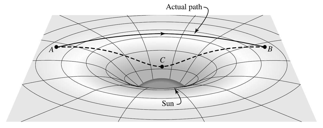
Fig. 3.1 Comparison of two photon paths through curved space between points \(A\) and \(B\). The path \(ACB\) is a straight line when projected onto a flat plane. Image Credit: Carroll & Ostlie (2007).#
Suppose we use a series of mirrors to force the light beam to trave between points \(A\) and \(B\) by the apparent “shortcut” of moving through the indentation of the Sun (see Fig. 3.1). Would the light taking this path outrace the beam free to follow its natural route around the curved space?
The answer is no–the curved beam would win the race. This result seems to imply that the beam following the “shortcut” would slow down along the way. However this can’t be correct because the postulates of special theory of relativity state that every observer observes the same speed of light. There are just two possible answers.
The distance along the “shortcut” path might actually be longer than the light beam’s natural path and/or
time might run more slowly along the dashed path.
Either answer would retard (slow down) the beam’s passage. According to general relativity, these effects contribute equally to delaying the light beam’s trip from \(A\) to \(B\). The curving light beam actually does travel the shorter path. If two space travelers were to lay meter sticks end-to-end along the two paths, the dashed path would require a greater number of meter sticks because it penetrates deeper into the curved space. In addition, the curvature of space involves an accompanying slowing down of time, so clocks placed along the dashed path would actually run more slowly. Therefore, time runs more slowly in curved spacetime.
As soon as Einstein competed his theory, he applied it to the problem of Mercury’s unexplained residual perihelion shift of \(43^{\prime\prime}\) per century.
Another triumph came in 1919 when the curving path of starlight passing near the Sun was first measured (by Sir Arthur Eddington) during a total solar eclipse. In this observation, the apparent positions of stars close to the Sun’s eclipsed edge were shifted from their actual positions by a small angle. Einstein’s theory predicted this angular deflection would be \(1.75^{\prime\prime}\), which is in good agreement with Eddington’s observations.
The superior conjunction of Mars that occurred in 1976 let to a spectacular confirmation of the theory. Radio signals beamed to Earth from the Viking spacecraft on Mars’ surface were delayed as they traveled through the curved spacetime surrounding the Sun. The time delay agreed with the predictions of general relativity to within \(0.1\%\).
3.1.2. The Principle of Equivalence#
One of the postulates of special relativity states that the laws of physics are the same in all inertial reference frames. Accelerating reference frames are not inertial, because the introduce fictitious forces that depend on the acceleration. For example, an apple at rest on the seat of a car will not remain at rest if the car suddenly brakes to a halt. However, the acceleration produced by gravity has a unique aspect.
Consider two massive, charged objects separated by a distance \(r\): one of mass \(m\) and charge \(q\), while the other is of mass \(M\) and charge \(Q\). The magnitude of the acceleration \(a_g\) of mass \(m\) due to the gravitational force is found from
while the magnitude of the acceleration \(a_e\) due to the electrostatic force is found from
The mass \(m\) (coupled on the left side with an \(a\)) is an inertial mass and measures the object’s resistance to being accelerated (i.e., its inertia). The masses (\(m\) and \(M\)) and charges (\(q\) and \(Q\)) on the right are numbers that couple the masses or charges to their respective forces and determine the strength of these forces. The mystery is the appearance of \(m\) on both sides of the formula.
Why should a quantity that measures an object’s inertia be the same as the “gravitational charge” that determines the force of gravity? Actually Eq. (3.2) is not properly written and should be expressed as
to distinguish between the inertial and gravitational mass of each object. Similarly, Eq. (3.3) should be
In this case the only mass that enters the expression is the inertial mass.
Experimentally, we have found that the ratio \(m_g/m_i\) is a constant to a precision of 1 part in \(10^{12}\) (i.e., 1 ppt). For convenience, this constant is chosen to be unity so that the two types of mass will be numerically equal.
If the gravitational mass were chosen to be twice the inertial mass, the laws of physics would be unchanged because the gravitational constant \(G\) would be assigned a new value that is only one-fourth as large. The proportionality of the inertial and gravitational masses means that, at a given location, all objects experience the same gravitational acceleration. The constancy of \(m_g/m_i\) is sometimes referred to as the weak equivalence principle.
The aspect of gravity in which every object falls with the same acceleration is not new and known since the time of Galileo. Einstein realized that if an entire laboratory were in free-fall, with all of its contents together, there would be no way to detect its acceleration. It would be impossible to experimentally determine whether the laboratory was floating in space (far from any massive object) or falling freely in a gravitational field. This posed a serious problem for the theory of special relativity, which requires that inertial frames have a constant velocity. An inertial frame cannot even be defined in the presence of gravity because it is equivalent to an accelerating laboratory.
The way to eliminate gravity in a laboratory is to surrender to it by entering into a state of free-fall. There was an obstacle to applying this to special relativity because its inertial reference frames are infinite collections of meter sticks and synchronized clocks. It would be impossible to eliminate gravity everywhere in an infinite, freely falling reference frame, because different points would have to be falling at different rates in different directions.
Einstein realized that he would have to use local reference frames, just small enough that the acceleration due to gravity would be essentially constant in both magnitude and direction everywhere inside the reference frame. Gravity would then be abolished inside a local, freely falling reference frame.
Note
Free-fall means that the only acceleration on the laboratory is due to gravity. John Wheeler suggested the term free-float, since gravity has been abolished, why should falling even be mentioned?
In 1907, Einstein adopted this as the cornerstone of his theory of gravity, calling it the principle of equivalence.
The Principle of Equivalence: All local, freely falling, nonrotating laboratories are fully equivalent for the performance of all physical experiments.
The restriction to nonrotating labs is necessary to eliminate the fictitious forces associated with rotation (e.g., the Coriolis and centrifugal forces). To simply the jargon: local, freely falling, nonrotating laboratories are called local inertial reference frames.
Note
Special relativity is incorporated into the principle of equivalence. For example, two measurements made from two local inertial frames in relative motion are related by the Lorentz transformations using the instantaneous value of the relative velocity between the two frames. As a result, general relativity is an extension of the theory of special relativity.
3.1.3. The Bending of Light#
Imagine an elevator suspended above the ground by a cable. A photon leaves a horizontal flashlight at the same instant the cable holding the elevator is cut. Gravity has been abolished from this freely falling elevator, so it is now a local inertial reference frame. According to the equivalence principle, an observer falling with the lab will measure the light’s path across the elevator as a straight horizontal line, in agreement with all of the laws of physics.
But another observer on the ground sees an elevator that is falling under the influence of gravity. The ground observer must measure a photon that falls with the elevator following a curved path. The curved path taken by the photon is the quickest route possible through the curved spacetime surrounding Earth (e.g., the rubber sheet analogy).
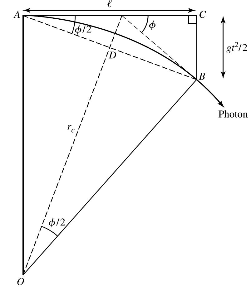
Fig. 3.2 Geometry for the radius of curvature \(r_c\) and angular deflection \(\phi\). Image Credit: Carroll & Ostlie (2007).#
The angle of deflection \(\phi\) of the photon is very slight. The photon does not follow a circular path, but we can use a best-fitting circle of radius \(r_c\) as an approximation of the path measured by the ground observer. The center of the best-fitting circle is at point \(O\), and the arc of the circle subtends an angle \(\phi\) between the radii \(OA\) and \(OB\). If the width of the elevator is \(\ell\), then the photon crosses the lab in time \(t=\ell/c\). In this amount of time, the lab falls a distance \(d=\frac{1}{2}gt^2\). Because triangles \(ABC\) and \(OBD\) are similar (i.e., contain a right angle and another angle \(\phi/2\))
Since \(\phi \ll 1\), we can set \(\cos{(\phi/2)}\simeq 1\) and the distance \(\overline{OD} \simeq r_c\). Substituting variables and solving for \(r_c\), we get for the radius of curvature for the photon’s path
using \(g=9.8\ \rm m/s^2\), which is nearly a light-year! If we assume that the width of the elevator \(\ell\) roughly equals the arclength of the curvature and \(\ell = 10\ \rm m\), then we can calculate \(\phi\)
or only \(2.25 \times 10^{-10}\ {\rm arcsec}\). The large radius of the photon’s path indicates that spacetime near Earth is only slightly curved. The curvature is still great enough to produce the circular orbits of satellites, which move slowly (compared to the speed of light) through the curved spacetime.
3.1.4. Gravitational Redshift and Time Dilation#
Returning to the elevator, but with a monochromatic light of frequency \(\nu_o\) leaving a vertical flashlight on the floor at the same instant the cable holding the elevator is cut. The freely falling elevator is again a local inertial frame, and so the equivalence principle requires that a frequency detector in the ceiling record the same frequency \(\nu_o\).
But an observer on the ground sees a lab that is falling under the influence of gravity. If the light has traveled upward a height \(h\) toward the meter in time \(t=h/c\), then the detector has gained a downward speed toward the light of \(v = gt = gh/c\). We would expect that in the ground observer’s frame, the detector should have measured a blueshifted frequency greater than \(\nu_o\). For the slow free-fall speeds involved, the expected increase in frequency is
However the detector records no change in frequency. Therefore, there must be another effect of the light’s upward journey through the curved spacetime around Earth that compensates for the blueshift exactly. This is a gravitational redshift that tends to decrease the frequency of the light as it travels upward a distance \(h\), which is exactly opposite the blueshift, or
An outside observer would measure only this gravitational redshift. If the light were traveling downward, a corresponding blueshift would be measured.
Exercise 3.1
In 1960, a test of the gravitational redshift formula was carried out at Harvard University. A \(\gamma\) ray was emitted by an unstable isotope of iron \(^{57}_{26}{\rm Fe}\) at the bottom of a tower \(22.6\ \rm m\) tall, and received at the top of the tower.
What is the expected gravitational redshift \(\Delta \nu/\nu_o\)?
From the gravitational redshift formula, we only need to know \(h\) because the acceleration due to gravity \(g\) is approximately constant (i.e., \(h\ll r_\oplus\)) and the speed of light is a known constant. Therefore, we find using \(h = 22.6\ \rm m\):
which is in excellent agreement with the experimental result of \(\frac{\Delta \nu}{\nu_o} = -(2.57 \pm 0.26) \times 10^{-15}\). More precise experiments carried out since have obtained agreement to within \(0.007\%\).
Note
The experiment was performed with both upward and downward traveling \(\gamma\) rays providing tests of both the gravitational redshift and blueshift.
An approximate expression for the total gravitational redshift for a light beam that escapes out to infinity can be calculated by integrating Eq. (3.7) from an initial position \(r_o\) to \(\infty\). Instead of using a constant acceleration due to gravity, we can use \(g = GM/r^2\) from Newtonian gravity and set \(h\) equal to the differential radial element \(dr\) for a spherical mass \(M\).
By integrating we are really adding up the redshifts obtained for a chain of different frames. The radial coordinate \(r\) can be used to measure distances for these frames if spacetime is nearly flat (i.e., \(r_c \gg r_o\)). In this case, the “stretching” of distances is not too severe, and we can integrate
where \(\nu_o\) and \(\nu_\infty\) are the frequencies at \(r_o\) and \(\infty\), respectively. The result
is valid when gravity is weak (i.e., \(r_o/r_c = GM/r_oc^2 \ll 1\)). This can be rewritten as
When the exponent \(x\) in \(e^{-x}\) is small (i.e., \(x \ll 1\)), we can use the approximation \(e^{-x} \simeq 1 - x\) to get
This approximation shows the first-order correction to the frequency of the photon. The exact result for the gravitational redshift (valid even for a strong gravitational field) is
The gravitational redshift can be incorporated into the redshift parameter (using Eq. (2.26)), giving
which is valid only for a weak gravitational field because we used the approximation \((1-x)^{1/2} \simeq 1-x/2\) for \(x\ll 1\).
To understand the origin of the gravitational redshift, imagine a clock that is constructed to tick once with each vibration of a monochromatic light wave. The time between ticks is then equal to the period of the oscillation of the wave \(\Delta t = 1/\nu\). The gravitational redshift implies that the clock at \(r_o\) will tick more slowly than an identical clock at \(r = \infty\). If an amount of time \(\Delta t_o\) passes at position \(r_o\) outside a spherical mass \(M\), then the time \(\Delta t_\infty\) at \(r=\infty\) is
using Eq. (2.26). For a weak field, this simplifies to
We must conclude that time passes more slowly as the surrounding spacetime becomes more curved, which is called gravitational time dilation. The gravitational redshift is therefore a consequence of time running at a slower rate near a massive object.
Exercise 3.2
The white dwarf Sirius B has a radius \(R = 5.8 \times 10^{6}\ {\rm m} = 0.0084\ R_\odot\) and a mass \(M = 2.026 \times 10^{30}\ {\rm kg} = 1.018\ M_\odot\).
(a) What is the radius of curvature \(r_c\) for a light beam near the surface?
(b) What is the gravitational redshift parameter \(z\) an emitted photon from the surface?
(c) What is the gravitational time dilation \((\Delta t_\infty - \Delta t_o)\) experienced by the photon as seen from a distant observer?
(a) The radius of curvature of a horizontally traveling light beam near the surface of Sirius B can be determined via Eq. (3.6),
using the given values for the mass and radius of Sirius B. Since \(R/r_c =2.57 \times 10^{-4} \ll 1\), the curvature is not severe and we can use the weak field approximation. Even at the surface of a white dwarf, gravity is considered relatively weak in terms of its effect on the curvature of spacetime.
(b) The gravitational redshift of a photon emitted from the surface can be calculated via the weak field approximation
This is in excellent agreement with the measured gravitational redshift for Sirius B (Joyce et al. 2018), where the percent error is only \({\sim}4.5\%\).
(c) To compare the rate at which time passes at the surface of Sirius B relative to a distant observer (i.e., \(r\rightarrow \infty\)), let’s suppose that exactly one hour is measured by a distant clock. The time recorded by a clock at the surface of Sirius B would be less than one hour using the weak field approximation:
The clock at the surface of Sirius B runs more slowly by about one second per hour compared to an identical clock far out in space.
from scipy.constants import G,c
import numpy as np

R_sun = 6.957e8 #radius of the Sun in m
M_sun = 1.99e30 #mass of the Sun in kg
R = 0.0084*R_sun #radius of Sirius B in m
M = 1.018*M_sun #mass of Sirius B in kg

#part a: Calculate the radius of curvature for Sirius B
r_c = (R*c)**2/(G*M)
print("part a: The radius of curvature r_c is %1.1e m." % r_c)
print("The parameter R/r_c is %1.3e." % (R/r_c))
print("--------------")
#part b: Calculate the gravitational redshift parameter z
#Using 0.01 as cutoff for weak field approximation
if R/r_c < 0.01:
    z = R/r_c
elif (2*R/r_c)<1:
    print("strong field")
    z = 1./np.sqrt(1-2*R/r_c) - 1
else:
    z = np.nan
    print("The radius of curvature can't be less than twice the stellar radius.")
print("part b: The gravitational parameter z is %1.1e." % z)
#measured z from (Joyce et al. 2018) https://academic.oup.com/mnras/article/481/2/2361/5090416
z_meas = 80.65e3/c
z_err = np.abs(z-z_meas)/z*100
print("The gravitational parameter z measured from HST is %1.1e, which gives an error of %2.1f percent." % (z_meas,z_err))
print("--------------")

#part c: Calculate the time dilation
dt_inf = 3600. #time measured by a distance clock (at infinity)
delta_t = dt_inf*(1-1./(z+1))
print("part c: The time dilation due to the curvature of spacetime is %1.2f s." % delta_t)
part a: The radius of curvature r_c is 2.3e+10 m.
The parameter R/r_c is 2.574e-04.
--------------
part b: The gravitational parameter z is 2.6e-04.
The gravitational parameter z measured from HST is 2.7e-04, which gives an error of 4.5 percent.
--------------
part c: The time dilation due to the curvature of spacetime is 0.93 s.
3.2. Intervals and Geodesics#
An event in spacetime unifies the concepts of space and time because it is expressed using four coordinates \((x,\ y,\ z,\ t)\). Einstein’s achievement was the deduction of his field equations for calculating the geometry of spacetime produced by a given distribution of mass and energy. His equations have the form
which depends on the stress-energy tensor \(\mathcal{T}\). The stress-energy tensor evaluates the effect of a given distribution of mass and energy on the curvature of spacetime. The appearance of the gravitational constant \(G\) and the speed of light \(c\) symbolizes the extension of special relativity to include gravity. It is beyond the scope of this course to explicitly evaluate this equation.
Note
Einstein’s field equations are similar to how Maxwell’s equations describe the changes in the electric or magnetic field due to the presence of charges.
3.2.1. Worldlines and Light Cones#
Spacetime diagrams represent a 2D physical plane \((x,\ y)\) with a perpendicular axis denoting time \(t\). The third spatial dimension \(z\) is ignored for simplicity. The path of an object as it moves through spacetime is called its worldline. Our task will be to calculate the worldline of a freely falling object in response to the local curvature of spacetime. The worldline’s spatial components can describe the trajectory of a baseball arcing toward an outfielder, a planet orbiting the Sun, or a photon attempting to escape a black hole.
Suppose a flashbulb is set off at the origin \((0,\ 0)\) at \(t=0\) and is designated as event \(A\). The worldlines of photons traveling in the \(x-y\) plane form a light cone that represents a widening series of circular slices through the expanding wavefront of light. By analogy, this is like the widening ripples of a disturbance in water projected along a third dimensions.

Fig. 3.3 Diagram of a light cone. A light cone (or “null cone”) is the path that a flash of light, emanating from a single event (localized to a single point in space and a single moment in time) and traveling in all directions, would take through spacetime. Image Credit: Wikipedia:light cone.#
A massive object initially at event \(A\) must travel slower than light, so the angle between its worldline and the time axis must be less than \(45^\circ\). The region inside the light cone represents the possible future of event \(A\). It consists of all the events possible for a traveler initially at rest at event \(A\). By extension, it also represents all the events that the traveler could every influence in a causal way.
Extending the diverging photon worldlines back through the origin generates a lower light cone. Within this light cone is the possible past of event \(A\), or the collection of all the events from whence a traveler could have arrived just as the bulb flashed. By extension, it contains all the events by which could have possibly caused the flashbulb to go off.
Outside the future and past light cones is an unknowable elsewhere, which is outside the ability of the traveler to receive or transmit information. In other words, the traveler cannot be influenced nor influence events that lie outside of his/her light cone. There are vast regions of spacetime that are hidden from us!
In principle, every event in spacetime has a pair of light cones extending from it. The light cone divides spacetime into that event’s future, past, and elsewhere. Two events can influence each other only if their light cones overlap in the past or future. Your entire future worldline (i.e., your destiny) must lie within your future light cone at every instant. Light cones represent horizons in space that separate the knowable from the unknowable.
3.2.2. Spacetime Intervals, Proper Time, and Proper Distance#
Measuring the progress of an object as it moves along its worldline involves defining a “distance” for spacetime. Consider two points (\(p_1\) and \(p_2\)) using 3D Cartesian coordinates
then the distance \(\Delta \ell\) measured along the straight line between two points in flat space is defined by
The analogous measure of “distance” in spacetime is called a spacetime interval (or interval). Let two events \(A\) and \(B\) have the spacetime coordinates
measured by an observer in an inertial reference frame \(S\). Then the interval \(\Delta s\) measured along the straight worldline between two events in flat spacetime is defined by
This definition of the interval is very useful because \((\Delta s)^2\) is invariant under a Lorentz transformation. An observer in another inertial reference frame \(S^\prime\) will measure the same value for the interval between two events \(A\) and \(B\) (i.e., \(\Delta s= \Delta s^\prime\)).
Note
The interval \((\Delta s)^2\) can be positive, negative or zero. The sign tells us whether the light has enough time to travel between two events.
If \((\Delta s)^2 > 0\), then the interval is timelike and light has more than enough time to travel between the two events. An inertial frame \(S\) can be chosen that moves along the straight worldline connecting events \(A\) and \(B\) so that the two events happen at the same location in \(S\). The time measured between the two events is \(\Delta s/c\). By definition, the time between two events that occur at the same location is the proper time \(\Delta \tau\), or
(3.16)#\[\begin{align} \Delta \tau \equiv \frac{\Delta s}{c}. \end{align}\]The proper time is the elapsed time recorded by a clock moving along the worldline from \(A\) to \(B\).
An observer in any inertial frame can use the interval to calculate the proper time between two events that separated by a timelike interval.
If \((\Delta s)^2 = 0\), then the interval is lightlike or null. In this case, light has exactly enough time to travel between events \(A\) and \(B\). Only light can make the journey from one event to the other, and the proper time along a null in is zero.
If \((\Delta s)^2 < 0\), then the interval is spacelike. Light does not have enough time to travel between events \(A\) and \(B\). No observer could travel between the events because a speed greater than \(c\) would be required.
The lack of absolute simultaneity in this situation, means that there are inertial reference frames in which the two events occur in the opposite temporal order, or even at the same time.
By definition, the distance measured between two events \(A\) and \(B\) in a reference frame for which they occur simultaneously (i.e., \(t_A = t_B\)) has a proper distance separating them,
If a straight rod were connected between the locations of the two events, this would be the rest length of the rod.
An observer in any inertial reference frame can use this to calculate the proper distance between two events that separated by a spacelike interval.
The interval is clearly related to the light cones.
The surfaces of the light cones (where the photons are at any time \(t\)), are the locations of all events \(B\) that are connected to \(A\) by a null interval.
The events within the future and past light cones are connect to \(A\) by a timelike interval, and
the events that occur elsewhere are connected to \(A\) by a spacelike interval.
3.2.3. The Metric for Flat Spacetime#
Obviously, a path connecting two points in 3D space doesn’t have to be straight. Two points can be connected by infinitely many curved lines. To measure the distance along a curved path \(\mathcal{P}\) from one point to the other, we use a differential distance formula called a metric:
The \(d\ell\) may be integrated along the path \(\mathcal{P}\) (e.g., using a line integral) to calculate the total distance between two points,
The distance between two points depends on the path connecting them. The shortest distance between two points in flat space is measured along a straight line, where the “straightest possible line” is when \(\Delta \ell\) is a minimum.
A worldline between two events in spacetime is not required to be straight either. To measure the interval along a curved worldline \(\mathcal{W}\) connecting two events in spacetime with no mass present, we use the metric for flat spacetime,
Note
There are two conventions for defining the metric: one where the space components have the \(-\), or the opposite (time component has the \(-\) and space components have a \(+\)). See the notes by Sean Carroll.
Then \(ds\) is integrated to determine the total interval along the worldline \(\mathcal{W}\),
The interval is still related to the proper time measured along the worldline.
For timelike worldlines, the proper time is \(\Delta \tau = \Delta s/c\).
For a null worldline, the proper time is zero.
For a spacelike worldline, the proper time is undefined.
In flat spacetime, the interval measured along a straight timelike worldline between two points is a maximum. Any other worldline between the same two events will not be straight and will have a smaller interval (i.e., \((c\ dt)^2 > (d\ell)^2\)). For a massless particle (e.g., a photon), all worldlines have a null interval \((\int \sqrt{(ds)^2}=0)\).
Suppose there are two events \(A\) and \(B\) that occur at times \(t_A\) and \(t_B\), respectively. The events are observed from an inertial reference frame \(S\) that moves from \(A\) to \(B\), chosen such that the two events occur at the origin of \(S\). The interval measured along the straight worldline connecting \(A\) and \(B\) is
Now consider the interval measured along another worldline connecting \(A\) and \(B\) that includes event \(C\), which occurs at \((x,\ y,\ z,\ t) = (x_C,\ 0,\ 0,\ t_C)\). In this case,
Using \(dx/dt = v_{AC}\) and \(dx/dt = v_{CB}\), for the constant velocity along worldline \(A\rightarrow C\) in the first integral and \(C\rightarrow B\) in the second integral, respectively, leads to
Thus, the straight worldline \((\Delta s(A\rightarrow B))\) has the longer interval. Any worldline connecting event \(A\) and \(B\) can be represented as a series of short segments, so we can conclude that the interval is indeed a maximum for the straight worldline.
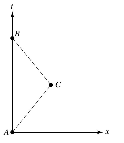
Fig. 3.4 Worldlines connecting events \(A\) and \(B\) Image Credit: Carroll & Ostlie (2007)).#
3.2.4. Curved Spacetime and the Schwarzschild Metric#
In a spacetime that is curved in the presence of mass, even the “straightest possible worldline” will be curved. These straightest possible worldlines are called geodesics. Just like circles are special cases of an ellipse, a straight worldline is a special geodesic in a flat spacetime.
In curved spacetime, a timelike geodesic between two events has either a maximum or minimum interval. The value of \(\Delta s\) along a timelike geodesic is an extremum, when compared with the intervals of nearby worldlines between the same two events.
A massless particle (e.g., a photon) follows a null geodesic. Einstein’s key realization was that the paths followed by freely falling objects through spacetime are geodesics. From this he develops three fundamental features in general relativity.
Mass acts on space time, telling it how to curve.
Spacetime in turn acts on mass, telling it how to move.
Any freely falling particle (including a photon) follows the straightest possible worldline (a geodesic) through spacetime. For a massive particle, the geodesic has a maximum or minimum interval, while for light the geodesic has a null interval.
For situations with spherical symmetry, it will be more convenient to use the familiar spherical coordinates \((r,\ \theta,\ \phi)\) instead of Cartesian coordinates. The metric between two nearby points in flat space is then
and the corresponding expression for the flat spacetime metric is
The specific situation to be investigated is the motion of a particle through the curved spacetime produced by a massive sphere (e.g., a planet, star, or a black hole). The first task is to calculate how this massive objects acts on spacetime, telling it how to curve. This requires a description of the metric.
Note
In a flat spacetime:
The variables \(r\), \(\theta\), \(\phi\), and \(t\) are the coordinates used by an observer at rest, a great (i.e., practically infinite) distance from the origin.
In the absence of a central mass at the origin, \(r\) would be the distance from the origin, and differences in \(r\) would measure the distance between points on a radial line.
The time \(t\) measured by clock scatter throughout the coordinate system would remain synchronized, advancing everywhere at the same rate.
In a curved spacetime around a massive sphere (mass \(M\) and radius \(R\)):
The origin (which is inside the sphere) should not be used as a point of reference (i.e., infinity at the origin). Instead imagine a series of nested concentric spheres centered at the origin.
The surface area of a sphere can be measured without approaching the origin, so the coordinate \(r\) will be defined by the surface of that sphere having an area \(4\pi r^2\).
As an object moves through the curved spacetime, its coordinate speed is just the rate of change of the spatial coordinates.
At large distances (\(r\simeq \infty\)), spacetime is essentially flat, and the gravitational time dilation of a photon is given by Eq. (3.12). The factor \(\sqrt{1-2GM/(rc^2)}\) plays a role in defining the metric. Recall that the stretching of space and the slowing down of time contribute equally to delaying a light bean’s passage through curved spacetime. The angular terms are the same as those for a flat spacetime.
In 1916, just two months after Einstein published his general theory of relativity, Karl Schwarzschild solved Einstein’s field equations (from the WWI trenches, where he died) to obtain a metric for the massive sphere:
which is now called the Schwarzschild metric.
It is important to realize that the Schwarzschild metric is the spherically symmetric vacuum solution of Einstein’s field equations. It is valid only in the empty space outside the object. The mathematical form is different in the object’s interior which is occupied by matter.
The Schwarzschild metric contains the “curvature of space” in the radial term. The radial distance measured simultaneously \((dt = 0)\) between two nearby points on the same radial line \((\theta = d\phi = 0)\) is just the proper distance (Eq. (3.17)),
The spatial distance \(d\mathcal{L}\) between two points on the same radial line is greater than the coordinate difference \(dr\) (i.e., the denominator must be less than unity). This represents the stretched grid lines in the rubber sheet analogy. The factor \(1/\sqrt{1-2GM/(rc^2)}\) must be included in any calculation of spatial distances.
Note
When using a topographic map to measure the distances along a steep trail, the elevation contour lines must be included in any calculation of the actual hiking distance. The same is true for measuring distances in a curved spacetime.
The Schwarzschild metric also incorporates time dilation and the gravitational redshift. If a clock is at rest at the radial coordinate \(r\), then the proper time \(d\tau\) it records is related to the time that elapses at an infinite distance by
Since \(d\tau < dt\), this shows that time passes more slowly closer to the massive sphere.
3.2.5. The Orbit of a Satellite#
General relativity shows us that a curved spacetime tells an orbiting particle of mass \(m\) how to move around a central massive object of mass \(M\). The rule is that it will follow the straightest possible worldline, the worldline with an extremal interval (assuming \(m\ll M\)).
According to Newton, the motion of a satellite in a circular orbit around Earth is found by simply equating the centripetal and gravitational accelerations, through
where \(v\) is the orbital speed.
Einstein and Newton must agree on the limiting case of weak gravity, so this result must come naturally from the Schwarzschild metric for curved spacetime (after some approximation). Using the Schwarzschild metric, we find that the straightest possible worldline is a circular orbit.
Determining the maximum interval between two fixed events requires applying the laws of conservation of energy, momentum, and angular momentum because they are built into Einstein’s field equations. However, a simpler strategy assumes that the satellite travels around the equator of the host body \((\text{polar angle, }\theta = 90^\circ)\) in a circular orbit with a specified angular speed \(\omega = v/r\). For a closed, unperturbed orbit, we find \(dr = 0\), \(d\theta = 0\), and \(d\phi = \omega dt\). Applying these conditions to the Schwarzschild metric (Eq. (3.22)) gives,
Integrating the spacetime interval for one orbit \((T = 2\pi/\omega = 2\pi r/v)\) is just
Since we assumed that the orbit is closed and unperturbed, we must be certain that the endpoints of the satellite’s worldline remain fixed (i.e., the satellites must begin and end at the same position \(r_o\) for all worldlines). The satellite can move (rapidly) radially outward from \(r_o\) to a radius \(r\), as long as the satellite returns just as rapidly to its starting point. The net effect is a purely circular motion.
In Eq. (3.25), the limits of integration are constant and the only variable is \(r\). The value of the radial coordinate actually followed by the satellite must be for which \(\Delta s\) is an extremum. Recall from Calculus that extremum are found by setting the first derivative to zero. Doing so produces,
The derivative may be taken inside the integral to obtain
Using \(v=r\omega\) allows us to write
which is the coordinate speed of the satellite for a circular orbit. This result is valid even for the very large spacetime curvature around a black hole!
Note
By coordinate speed, we mean that \(v = r\ d\phi/dt\) is the speed of the satellite measured in the \((r,\ \theta,\ \phi,\ t)\) coordinate system by a distant observer.
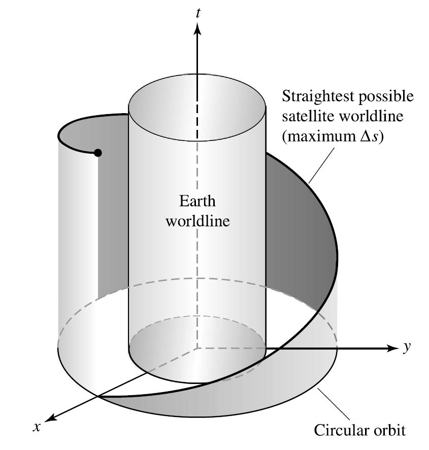
Fig. 3.5 The straightest possible worldline through curved spacetime and its projection onto the orbital plane of the satellite. Image Credit: Carroll & Ostlie (2007).#
3.3. Black Holes#
In 1783, John Michell considered the implications of Newton’s corpuscular theory of light, where light exists as a stream of particles. Michell reasoned that this stream of particles should be influenced by gravity and a star with 500 times more gravity than the Sun (keeping the average density constant) would be sufficiently strong to prevent light from escaping it. The escape velocity of Michell’s star would be the speed of light.
Naively, we can use the Newtonian formula for the escape velocity equal to c to show that
is the radius of a star whose escape velocity equals the speed of light. Using the mass of the Sun, \(R = 2.95(M/M_\odot)\ {\rm km}\). The resulting radius of such a star seemed unrealistically small, and so it held little interest for astronomers until the mid 1900s.
In 1939, J. Robert Oppenheimer and Hartland Snyder described the ultimate gravitational collapse of a massive star that exhausted its sources of nuclear fusion. Oppenheimer and Snyder pursued the question of the fate of a degenerate star that might exceed this limit and surrender completely to the force of gravity. See Oppenheimer & Snyder 1939 for more details.
3.3.1. The Schwarzschild Radius#
For the simplest case of a nonrotating star, we can estimate the radius of an object where gravity dominates over light. The answer lies in the Schwarzschild metric (Eq. (3.22)), where the time and radial terms have a common factor
To find the limiting radius, we simply identify when the square root in the metric goes to zero:
where \(R_S\) is the Schwarzschild radius. The behavior at the Schwarzschild radius (i.e., \(r=R_S\)) is bizarre, where the proper time is \(d\tau = 0\). Time has slowed to a complete stop, as measured by a distant observer. Nothing ever happens at the Schwarzschild radius!
Does it imply that even light is frozen in time? The speed of light measured by an observed suspended above the collapsed star must always be \(c\). A distant observer can determine that the light is delayed as it moves through curved spacetime. The apparent speed of light (i.e., the rate of change for the spatial coordinates of a photon) is called the coordinate speed of light. For a radially moving photon (i.e., \(d\theta = d\phi = 0\)), we can determine the coordinate speed of light suing the Schwarzschild metric (with \(ds=0\)) as
When \(r\gg R_S\), then \(dr/dt \simeq c\), as expected in flat spacetime. However, at \(r=R_S\), \(dr/dt = 0\) (see Fig. 3.6 and its python code for implementation). Light is indeed frozen in time at the Schwarzschild radius. The spherical surface at \(r=R_S\) acts as a barrier and prevents any information to flow outward from within.
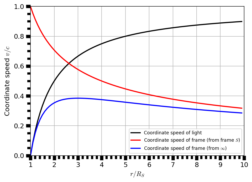
Fig. 3.6 The coordinate speed from the reference of the photon (black), the reference frame \(S\) (red), and from a freely falling distant observer at infinity (blue).#
import numpy as np
import matplotlib.pyplot as plt
from matplotlib import rcParams
from myst_nb import glue

rcParams.update({'font.size': 14})
rcParams.update({'mathtext.fontset': 'cm'})

fs = 'large'
r = np.arange(1,10,0.1) #radius r relative to the Schwarzschild radius R_s

v_light = 1. - 1./r #Coordinate speed of light
v_S = np.sqrt(1/r) #Coordinate speed of frame seen from S
v_inf = v_light*v_S #Coordinate speed of frame seen from infinity

fig = plt.figure(figsize=(7,5),dpi=150)
ax = fig.add_subplot(111)

ax.plot(r,v_light,'k-',lw=2,label="Coordinate speed of light")
ax.plot(r,v_S,'r-',lw=2,label="Coordinate speed of frame (from frame $S$)")
ax.plot(r,v_inf,'b-',lw=2,label="Coordinate speed of frame (from $\infty$)")

ax.legend(loc='best',fontsize='small')
ax.minorticks_on()
ax.tick_params(which='major',axis='both', direction='out',length = 8.0, width = 6.0,labelsize=fs)
ax.tick_params(which='minor',axis='both', direction='out',length = 6.0, width = 4.0)
ax.grid(True)

ax.set_xlabel("$r/R_S$",fontsize=fs)
ax.set_ylabel("Coordinate speed $v/c$",fontsize=fs)
ax.set_xlim(1,10)
ax.set_ylim(0,1)


glue("coordinate_speed_fig", fig, display=False);
For this reason, a star that has collapsed down within the Schwarzschild radius is called a black hole. It is enclosed by the event horizon, which is a spherical surface at \(r=R_S\).
Although the interior of a black hole is a region that is forever hidden from us, its properties can still be calculated. A nonrotating black hole has a singularity (i.e., a point of zero volume and infinite density) at the center, where all the black hole’s mass is located. Spacetime is infinitely curved at the singularity. Cloaking the central singularity is the event horizon, where there is a hypothesis dubbed the Law of Cosmic Censorship that forbids a naked singularity from appearing without an associated event horizon (i.e., unclothed).
3.3.2. A Trip into a Black Hole#
Imagine an attempt to investigate the black hole by starting a safe distance and reflecting a radio wave from an object at the event horizon. How much time will it take for a photon to reach the event horizon from a radial coordinate \(r\gg R_S\) and then return?
Since the roundtrip is symmetric, it is necessary to only determine half of the journey and double the result. It is easiest to integrate the coordinate speed of light in the radial direction (Eq. (3.28)) between two arbitrary values of \(r_1\) and \(r_2\) to obtain
assuming that \(r_1< r_2\). Inserting \(r_1 = R_s\) for the photon’s original position, we find that \(\Delta t = \infty\). The radio photon will never reach the event horizon. Instead the photon’s coordinate velocity will slow down until it finally stops at the event horizon in the infinite future. Any object falling toward the event horizon will suffer the same fate. In a sense, a black hole is a frozen star because the surface of the event horizon appears frozen from the outside.
A brave (and indestructible) astronomer decides to start from rest at a great distance, and fall freely toward a \(10\ M_\odot\) black hole (\(R_s\simeq 30 {\rm km}\)). The astronomer’s local inertial frame \(S\) falls with a coordinate speed \(dr/dt\) all the way to the event horizon. During the acceleration, a monochromatic flashlight sends a pulse of photons in our direction once per second. As the infall progresses, the light signals arrive farther and farther apart for several reasons:
Subsequent signals must travel a longer distance as the astronomer accelerates. The proper time \(\tau\) is running more slowly than our coordinate time \(t\) from the location (gravitational time dilation) and motion (special relativity time dilation) of the astronomer.
The coordinate speed of light becomes slower as the astronomer approaches the black hole, so the signals travel back to us more slowly.
The frequency of light waves we receive is increasingly redshifted. This is cased by the astronomer’s acceleration away from us and the gravitational redshift. The redshifted light may be in a range that is not optimal for our detector.
The light becomes dimmer as the rate at which the flashlight pulses decreases and the energy per photon \((hc/\lambda)\) declines.
At about \(2\ R_S\) from the event horizon, the time between signals begins to increase without limit as the strength of the signals decreases. The astronomer is frozen in time.
How does all of this appear from the astronomer’s frame? Because gravity is abolished in the local frame, initially the approach to the black hole goes unnoticed. The astronomer’s watch displays the proper time \(\tau\), from which the flashlight pulses are timed.
However, the astronomer begins to feel stretched in the radial direction and compressed in the perpendicular direction. The gravitational pull on the astronomer’s feet (nearer to the black hole) is stronger than on the astronomer’s head. The variation in the direction of gravity from side to side produces a compression that is even more severe. The differential tidal forces increase in strength as the astronomer approaches the event horizon. The size of the local frame (where gravity is abolished) becomes smaller as the spatial variation in the gravitational acceleration vector increases. this is why the astronomer need be indestructible, because the tidal force would tear the astronomer apart at a distance of several hundred kilometers from the black hole.
In just \(2\ \rm ms\) (proper time), the astronomer falls the final few hundred kilometers to the event horizon and crosses it. It is impossible for any particle to be at rest when \(r < R_S\), as can be seen from the Schwarzschild metric (Eq. (3.22)). The interval can be calculated for an object at rest (i.e., \(dr=d\theta=d\phi=0\)) by
when \(r<R_S\). This is a spacelike interval that is not permitted for particles. Therefore it is impossible to remain at rest. Within the event horizon of a nonrotating black hole, all world lines converge a the singularity. Even photons are pulled in toward the center.
To see an object, you need to bounce photons off of the object and detect them with your retinas. If the photons are pulled toward the center, then they can’t make the return trip for you to detect them. This means that the astronomer never has an opportunity to glimpse the singularity. Although the elapsed coordinate time in the outside world does become infinite, the light from all of these events does not have time to read the astronomer. Instead, the events occur outside the astronomer’s light cone (in the elsewhere). See more detail in Rothman et al. (1985).
3.3.3. Mass Ranges of Black Holes#
Black holes appear to exist within a range of masses.
Stellar-mass black holes (\({\sim}3-15\ M_\odot\)) may from directly or indirectly as a consequence of the core-collapse of a sufficiently massive supergiant star.
The direct collapse of the core to a black hole may be responsible for the production of collapsar, whereas a delayed collapse of a rapidly rotating neutron star may result in a supranova (Vietri & Stella (1998)).
It is also possible that a neutron star in a close binary system may gravitationally strip enough mass from its companion that the neutron’s self-gravity exceeds the ability of the degeneracy pressure to support it, resulting in a black hole.
Intermediate-mass black holes (IMBHs) may exist from \(100\ M_\odot\) to \(>10^3-10^4\ M_\odot\).
Evidence for them exists in the detection of ultraluminious X-ray sources (ULXs) with space telescopes Chandra and XMM-Newton.
It is not clear how these objects might form, although correlation of IMBHs with the cores of globular clusters and low-mass galaxies suggests that they develop through mergers of stars (to form supermassive stars that undergo core-collapse), or by the merger of stellar-mass black holes.
Supermassive black holes (SMBHs) range in mass from \(10^5-10^9\ M_\odot\) and lie at the centers of many galaxies (probably most). Our own Milky Way Galaxy has a central black hole of mass \(M = (3.7 \pm 0.2) \times 10^6\ M_\odot\).
How these behemoths formed remains an open question. One popular suggestion is that they formed from galaxy collisions. Another is that they formed as an extension of the IMBH formation process.
SMBHs appear to be closely linked with some bulk properties of galaxies, implying an important connection between galaxy formation and the formation of SMBHs.
Primordial black holes may have been manufactured in the instants of the universe and may range from \(10^{-8}\ {\rm kg}\) to \(10^5\ M_\odot\).
Exercise 3.3
If Earth could somehow be compressed sufficiently to become a black hole:
What would be its Schwarzschild radius?
The Schwarzschild radius of any object can be computed using
where we substitute \(M_\oplus = 5.972 \times 10^{24}\ {\rm kg}\) for the \(M\) in the above equation. This results in
Although a primordial black hole could be this size, it is almost impossible to imagine packing Earth’s entire mass into so small a ball.
from scipy.constants import c, G

M_Earth = 5.972e24 #Earth mass in kg
R_S = 2*G*M_Earth/c**2
print("The Schwarzschild radius R_S for an Earth-mass object is %1.3e m." % R_S )
The Schwarzschild radius R_S for an Earth-mass object is 8.870e-03 m.
3.3.4. Black Holes Have No Hair!#
The formation of black holes are probably complicated, where the core-collapse of a star is almost certainly not symmetrical. Detailed calculations have demonstrated that any irregularities are radiated away by gravitational waves. Once the surface of collapsing star reaches the event horizon, the exterior spacetime horizon is spherically symmetric and described by the Schwarzschild metric.
Another complication is the fact that stars rotate, and therefore so will the resulting black hole. Remarkably, any black hole can be completely described by just three numbers: its mass, angular momentum, and electric charge. Black holes have no other attributes or adornments, a condition commonly expressed by saying that “a black hole has no hair”.
There is a firm upper limit for a rotating black hole’s angular momentum given by
If the angular momentum of a rotating black hole were to exceed this limit, there would be no event horizon and a naked singularity would appear (in violation of the Law of Cosmic Censorship).
Exercise 3.4
The mass of the Sun is \(M_\odot = 1.989 \times 10^{30}\ \rm kg\) and its angular momentum is \(L_{\rm Sun} = 1.63 \times 10^{41}\ {\rm kg\ m^2/s}\). Note that the subscript \(\rm Sun\) is used so that one is not confused by the notation of a solar luminosity \(L_\odot\).
What is the maximum angular momentum for a solar-mass black hole and how does it compare with \(L_{\rm Sun}\)?
The maximum angular moment for a solar-mass black hole is
The Sun’s current angular momentum is \(L_{\rm Sun} = 0.18 L_{\rm max}\), or 18% of the maximum value. Many stars will have angular momenta that are comparable to \(L_{\rm max}\), and fast rotation ought to be common for stellar-mass black holes.
from scipy.constants import c, G

M_odot = 1.989e30 #mass of the Sun in kg
L_sun = 1.63e41 #angular momentum of the Sun in kg m^2/s
L_max = (G*M_odot**2)/c
print("The maximum angular momentum of a solar-mass black hole is %1.2e kg m^2/s." % L_max)
print("The Sun's current angular momentum is %i percent of this maximum value." % (L_sun/L_max*100))
The maximum angular momentum of a solar-mass black hole is 8.81e+41 kg m^2/s.
The Sun's current angular momentum is 18 percent of this maximum value.
3.3.5. Spacetime Frame Dragging#
The structure of a maximally rotating black hole (see Fig. 3.7) distorts the central singularity from a point into a flat ring, and the event horizon assumes an ellipsoid shape. As a massive object spins, it induces a rotation in the surrounding spacetime, which is known as frame dragging. The Kerr metric is used to describe rotating black holes, which was derived from Einstein’s field equations by Roy Kerr in 1963.

Fig. 3.7 The boundaries of a Kerr black hole relevant to astrophysics. Note that there are no physical “surfaces” as such. The boundaries are mathematical surfaces, or sets of points in spacetime, relevant to analysis of the black hole’s properties and interactions. Image Credit:[Wikipedia:Rotating_black_hole].#
Recall the behavior of a pendulum swinging at the north pole of Earth. As Earth rotates, the plane of the pendulum’s swing remains fixed with respect to the distant stars. The stars define a nonrotating reference frame for the universe, and it is relative to this frame that the pendulum’s swing remains planar.
However, the rotating spacetime close to a massive spinning object produces a local deviation from the nonrotating frame. Near a rotating black hole, frame dragging is so severe that there is a nonspherical region outside the event horizon called the ergosphere, where any particle must move in the same direction as the black hole rotates. Spacetime within the ergosphere is rotating so rapidly that a particle’s speed would exceed the speed of light to remain at the same angular coordinate (i.e., at the same \(\phi\) for a distant observer). The outer boundary of the ergosphere is called the static limit, where a particle can remain at the same coordinate as the effect of frame dragging diminishes.
Even Earth’s rotation produces very weak frame dragging. Detecting the effect of frame dragging was the mission of the Stanford Gravity Probe B experiment. The polar-orbit spacecraft (from April 2004–October 2005) employed four superconducting gyroscopes made of precisely shaped spheres of fused quartz (\(3.8\ \rm cm\) in diameter). The gyroscopes were so nearly freely rotating that they formed an almost perfect spacetime reference frame.
Although the predicted precession rate of the gyroscopes was only \(0.042\ ^{\prime\prime}{\rm /yr}\), the effect of frame dragging is cumulative. The experiment measured the effect due to the this precision to \(20\%\) precision, where other experiments measured the effect down to \(10\%\) precision (see an article from Science for more detail.)
Note
The previous descriptions of a black hole’s interior structure are based on vacuum solutions to Einstein’s field equations. These solutions ignored the effects of the collapsing star’s mass, so the vacuum solutions do not describe the interior of a real black hole. The present laws of physics (including general relativity) break down under the extreme conditions found very near the center. The details of the singularity cannot be fully described until a theory of quantum gravity is found.
3.3.6. Tunnels in Spacetime#
A common trope in science fiction is to use a black hole as a means of connection two distant points in space time. Most conjectures on spacetime tunnels are based on vacuum solutions to Einstein’s field equations and don’t apply to real black hole interiors. Figure 3.8 shows a spacetime tunnel called a Schwarzschild throat (aka Einstein-Rosen bridge), which uses a Schwarzschild geometry (nonrotating black hole) to connect two regions of spacetime.
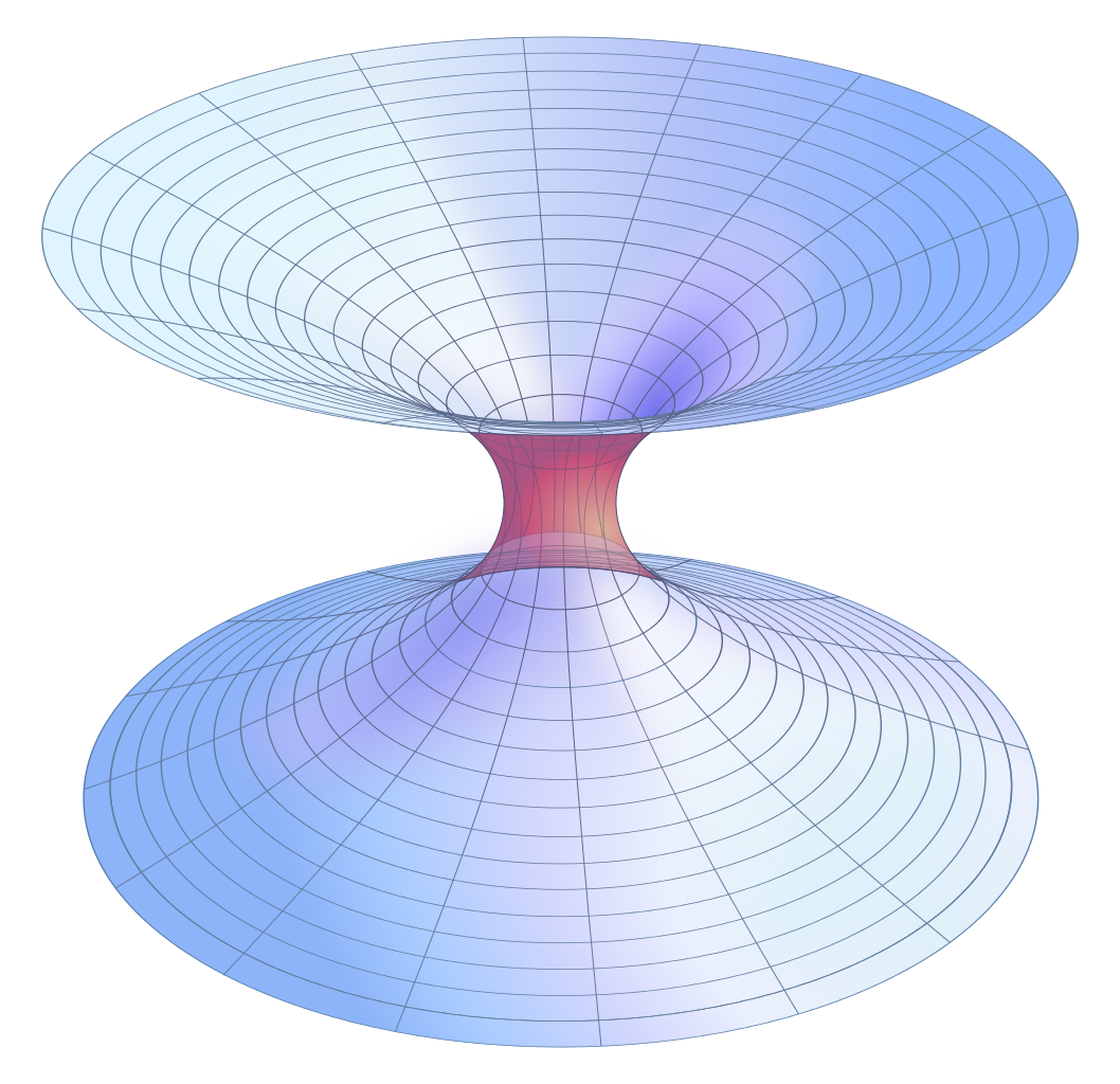
Fig. 3.8 “Embedding diagram” of a Schwarzschild wormhole. Image Credit:Wikipedia:Wormhole.#
The width of the throat is a minimum at the event horizon, and the “mouths” may be interpreted as opening onto two different locations in spacetime. It is tempting to imagine this as a tunnel, however it appears that any attempt to send a tiny amount of matter or energy through the throat would cause it to collapse. For a real nonrotating black hole, all worldlines end at the singularity, where spacetime is infinitely curved.
The story is somewhat different for a rotating black hole. Spacetime is still infinitely curved at the singularity, but all worldlines need not converge there. It is difficult for an infalling object to hit the singularity in a rotating black hole. There are vacuum solutions that miss the singularity and emerge in the spacetime elsewhere, but any attempt to pass the smallest amount of matter (or energy) along such a route would cause the passageway to collapse (i.e., pinching it off). For more realistic situations, any voyager attempting a trip through a black hole would end up being torn apart by the singularity.
Another possibility is a wormhole, which are similar to a Schwarzschild throat but are described by nonvacuum solutions to Einstein’s field equation. A wormhole must be threaded by some sort of exotic material whose tension prevents the collapse of the wormhole. There is no known mechanism that would allow a wormhole to arise naturally.
The problem with the exotic material required is that it must be capable of gravitationally defocusing light through an “antigravity” effect involving gravitational repulsion of the light. Exotic material meeting this requirement would have a negative energy density (\(\rho c^2 < 0\)), at least as experienced by the light rays. A negative energy density is allowed in certain quantum situations, it may (or may not) be allowed physically macroscopic scales.
3.3.7. Stellar-Mass Black Hole Candidates#
Extraordinary claims require extraordinary evidence (or the Sagan Standard) and proof of the mere existence of black holes has been difficult to obtain. The problem lies in detecting an object only a few tens of kilometers across that emits no radiation directly. The best hope for astronomers is to find a black hole in a close binary system. If the black hole in such a system is able to pull gas from the envelope of the normal companion (or red giant) star, then the angular momentum of their orbital motion would cause a gas disk to form around the black hole.
As the gas spirals down toward the event horizon, it is compressed and heated to millions of kelvins, thereby emitting X-rays. Only the gravity of a neutron star or black hole can produce X-rays in a close binary system. If an X-ray binary can be found in which the mass of the compact object exceeds \(3\ M_\odot\), then a strong case can be made that the compact object is a black hole.
Twenty-two X-ray binaries have been detected in our Milky Way galaxy and its nearest neighbor the Large Magellanic Cloud. The video below provides a visualization of these black hole systems, including the first suspected black hole system, Cynus X-1 (see NASA for more details).
The earliest black hole binary candidates were found using radial velocity measurements and Doppler-shifted spectral lines. A simple application of Kepler’s laws showed that the mass of the compact object in A0620-00 must be at least \(3.82 \pm 0.24\ M_\odot\), which is well above the \(3\ M_\odot\) upper limit for a neutron star.
V404 Cyngi was originally determined to be a recurrent nova, where V404 Cyg underwent an X-ray outburst in 1989. Examination with ground-based optical telescopes revealed a K0 IV companion star with a radial velocity amplitude of \(211 \pm 4\ \rm km/s\) and an orbital period of \(6.473 \pm 0.001\ \rm d\). It is also the first black hole with an accurate parallax measurement from the Solar System.
The Laser Interferometer Gravitational-Wave Observatory (LIGO) reported the detection (in 2016) of a pair of black holes using gravitational waves. However, these black holes were \({\sim}30\ M_\odot\) each and the merger took place about 1.3 billion light-years from Earth. Nearly 100 black hole mergers have been discovered since LIGO came back online in 2015. As a result, new theories have emerged about how black holes merge and grow into heavyweights (see this press release for more details).
3.3.8. Hawking Radiation#
The black holes of classical general relativity last forever, where a very general result by Stephen Hawking states that the surface area of a black hole’s event horizon can never decrease. If a black hole coalesces with any other object, the result is an even larger black hole.
In 1974, Hawking discovered that black holes can slowly evaporate when he combined quantum mechanics with the theory of black holes. The key to this process is pair production (i.e., formation of particle-antiparticle pairs) just outside the event horizon of a black hole. Ordinarily, the particles quickly recombine and disappear, but if one of the particles falls into the event horizon while its partner escapes, the disappearing act may be thwarted.
The black hole’s gravitational energy was used to produce the particles, and so the escaping particle carried away some of the black hole’s mass. The net effect (as seen by an observer at a great distance) is the emission of particles by the black hole, known as Hawking radiation, accompanied by a reduction in the black hole’s mass.
The rate at which energy is carried away by particles is inversely proportional to the square of the black hole’s mass (or \(1/M^2\)). For stellar-mass black holes, the emitted particles are photons and the emission rate is miniscule. As the black hole’s mass declines, the emission rate increases. The final stage of a black hole’s evaporation proceeds extremely rapidly, releasing a burst of all types of elementary particles.
The lifetime of a primordial black hole prior to its evaporation \(t_{\rm evap}\) is quite long,
Since the age of the universe is \(13.7 \times 10^9\ \rm yr\), this process is of no consequence for black holes formed by a collapsing star. A primordial black hole with a mass of roughly \(1.7 \times 10^{11}\ \rm kg\) (\({\sim}\) a small asteroid) would evaporate in about 13 billion years.
The final burst of Hawking radiation is thought to release high-energy (\(\approx 100\ \rm MeV\)) gamma rays at a rate of \(10^{13}\ \rm W\), together with electrons, positrons, and many other particles. The subsequent decay of these particles should produce additional gamma rays that would be observable by space-based gamma observatories. To date, the measurements of the cosmic gamma-ray background at this energy have not detected anything that can be identified with the demise of a nearby primordial black hole.
3.4. Homework#
Problem 1
A photon near the surface of Earth travels a horizontal distance of \(1\ \rm km\). How far does the photon “fall” in this time?
Problem 2
Estimate the radius of curvature of a horizontally traveling photon at the surface of a \(1.4\ M_\odot\) neutron star, and compare the result with the \(10\ \rm km\) radius of the star. Can general relativity be neglected when studying the neutron stars?
Problem 3
\(\tau\) Ceti is the closest single star that is Sun-like. At time \(t=0\), Alice leaves Earth in her starship and travels at a speed of \(0.95c\) to \(\tau\) Ceti. Her twin brother Bob, remains at home.
(a) According to Bob, what is the interval between Alice’s leaving Earth and arriving at \(\tau\) Ceti?
(b) According to Alice, what is the interval between her leaving Earth and arriving at \(\tau\) Ceti?
(c) Upon arriving at \(\tau\) Ceti, Alice immediately turns around and returns to Earth at the same speed (\(0.95c\)). What was the proper time for Alice during her round trip to \(\tau\) Ceti?
(d) When Alice and Bob are reunited on Earth, how much younger will Alice be than her brother?
Problem 4
Consider four black holes with masses of \(10^{12}\ \rm kg\), \(10\ M_\odot\), \(10^5\ M_\odot\), and \(10^9\ M_\odot\).
(a) Calculate the Schwarzschild radius for each.
(b) Calculate the average density, defined by \(\rho = M/(\frac{4}{3}\pi R_S^3)\), for each.
Problem 5
It can be shown that the orbit of a massive particle orbiting a nonrotating black hole is not stable unless \(r \geq 3 R_S\), where any disturbance will cause a particle in a smaller orbit to spiral down to the event horizon. For a \(10\ M_\odot\) black hole, and using
(a) Find the coordinate speed of a particle in the smallest stable orbit.
(b) Find the orbital period (in coordinate time \(t\)) for this smallest stable orbit.