The Milky Way Galaxy
Contents
5. The Milky Way Galaxy#
5.1. Counting the Stars in the Sky#
Humans have peered into the heavens and contemplated its vastness. Sometimes, we have proposed various models to explain its form. In some civilizations, the stars were believed to be on a celestial sphere that rotated majestically above a fixed, central Earth (i.e., geocentrism of Ptolemy). When Galileo made his first telescopic observations, we started down a long road that has dramatically expanded our view of the universe.
it is possible to get at least a general idea about the nature of other galaxies by studying our own Galaxy, but this is very challenging. We live in a disk of stars, dust, and gas that severely impacts our ability to “see” beyond our relative stellar neighborhood when we look along the plane of the disk. The problem is most severe when looking toward the center of the Galaxy in the constellation Sagittarius.
Much of what we know today about the formation and evolution of the Milky Way is encoded in the motions of the Galaxy’s constituents, especially when combined with information about the variations in composition. Unfortunately, measuring the motions of the stars and gas in the Galaxy is done from a moving observing platform (i.e., the Earth) that is undergoing another motion around the Sun, which is orbiting the Galactic center.
5.1.1. Historical Models#
From observations of a dark night sky, an almost continuous band of light appears to circle the Earth. It is inclined by about \(60^\circ\) with respect to the celestial equator. It was Galileo who first realized that this Milky Way is a vast collection of individual stars. In the mid-1700s, Kant and Wright proposed that the Galaxy must be a stellar disk and our Solar System is merely one component within that disk. In the 1780s, William Herschel produced a map of the Milky Way based crudely on counting the number of stars the he could observe in 683 regions of the sky. In his analysis, Herschel assumed that
all stars have approximately the same absolute magnitude,
the number density of stars in space is roughly constant,
there is nothing between the stars to obscure them, and
he could see the edges of the stellar distribution.
From his data, Herschel concluded that the Sun had to be very near the center of the distribution and that the dimensions measured along the plane of the disk were some \(5\times\) greater than the disk’s vertical thickness.
Fig. 5.1 William Herschel’s map of the Milky Way Galaxy based on star counts. Image Credit:Edward Wright @ UCLA.#
Jacobus Kapteyn confirmed Herschel’s model of the Galaxy, again using the technique of star counting. Through the use of more quantitative methods, Kapteyn was able specify a distance scale for his model of the Galaxy. The Kapteyn universe was a flattened spheroidal system with a steadily decreasing stellar density with increasing distance from the center.
In the plane of the Galaxy and at a distance of some \(800\ \rm pc\) from the center, the number density of stars had decreased from its central value by a factor of \(2\). On an axis passing through thecenter and perpendicular to the central plane, the number density decreased by \(50\%\) over a distance of only \(150\ \rm pc\). The number density diminished to \(1\%\) of its central value at distances of \(8500\ \rm pc\) (in the plane) and \(1700\ \rm pc\) (perpendicular to the plane). Kapteyn concluded that the Sun was located \(38\ \rm pc\) north of the Galactic midplane and \(650\ \rm pc\) from the center, measured along the Galactic midplane.
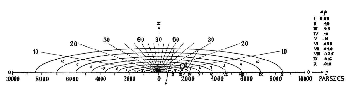
Fig. 5.2 The Kapteyn universe, where surfaces of constant stellar number density are indicated around the Galactic center. Image Credit: Carroll & Ostlie (2007); Figure from Kapteyn (1922).#
To follow Kapteyn’s logic for his nearly heliocentric model of the universe, recall the equation for the distance modulus:
Assuming a value for \(M\) (e.g., if the spectral class and luminosity class are known) and measuring \(m\) at a telescope, the distance modulus \(m-M\) and the distance \(d\) are readily obtained. Given the known coordinates of the star on the celestial sphere, its 3D position relative to the Earth is determined.
In actuality, it is impractical to estimate the distance to each individual star in the way described above because the number of stars in any given region is so great. Instead, a statistical approach is used that is based on counting the number of stars in specified region down to a predetermined limiting apparent magnitude. From this counting procedure, the number density of stars at a given distance can be estimated.
Shortly before Kapteyn’s model was published, Harlow Shapley estimated the distances to 93 globular clusters using RR Lyrae and W Virginis stars. These stars are easily identified in the clusters through their periodic variations in luminosity, and it is a matter of using the period-luminosity relation (to get their absolute magnitudes) to estimate their distances from the Sun. The distances to the variable stars correspond to the distances to the clusters in which they reside.
Shapley recognized that the globular clusters are not distributed uniformly throughout space, but are found preferentially in a region of the sky that is centered in the constellation of Sagittarius, at \(15\ \rm kpc\) from the Sun. He estimated that the most distant clusters are more than \(70 \rm kpc\) form the Sun, over \(55\ \rm kpc\) from the center. As a result, Shapley believed that the diameter of the Galaxy was on the order of \(100 \rm kpc\), which is close to \(10 \times\) the diameter estimated by Kapteyn.
Today, we known that Kapteyn’s universe was too small and the Sun was too near the center, and Shapley’s Galactic model was too large. Both models errored in part for the same reason:
the failure to include in their distance estimates the effects of interstellar extinction due to gas and dust.
Kapteyn’s selected regions were largely within the Galactic disk where extinction effects are most severe; as a result, he was unable to see the most distant portions of the Milky Way (causing him to underestimate its size). The problem is analogous to someone on Earth trying to see the surrounding land while standing in a dense fog with limited visibility.
Shapely chose to study objects that are generally found well above (and below) the plane of the Milky Way, and are inherently bright, which makes them visible from great distances. It is in directions perpendicular to the disk that interstellar extinction is least important, although it cannot be neglected entirely. Errors in the calibration of the period-luminosity relation used by Shapely let to overestimates of the distances to the clusters. The calibration errors were traced to the effects of interstellar extinction.
Kapteyn was aware of the errors that interstellar extinction could introduce but he was unable to find any quantitative evidence for the effect. Other researchers at the time suspected that dust might be responsible for the dark bands running across the Milky Way.
Further evidence for strong extinction could also be found in Shapely’s own data. No globular clusters were visible within a region between approximately \(\pm 10^\circ\) of the Galactic plane called the zone of avoidance. Shapely suggested that globular clusters were apparently absent in the zone of avoidance because strong gravitational tidal forces disrupted the objects in that region; this was a similar argument for the existence of the Asteroid Belt in the Solar System. In reality, interstellar extinction is so severe within the zone of avoidance that the very bright clusters are simply undetectable.
5.1.2. The Effects of Interstellar Extinction#
To see how interstellar extinction directly affects the estimates of stellar distances, we find
where \(d^\prime = 10^{(m_\lambda - M_\lambda + 5)/5}\) is the erroneous estimate of the distance when extinction is neglected, and \(A_\lambda\) is the amount of extinction in magnitudes. The extinction coefficient and magnitudes (\(M\) and \(m\)) are all a function of wavelength due to the wavelength dependent way that light is scattered (or blocked) by dust or absorbed by gas clouds. Since \(A_\lambda \geq 0\) in all cases (i.e., extinction can’t make a star appear brighter), \(d\leq d^\prime\); the true distance is always less than the apparent distance.
In the disk of the Milky Way, the typical extinction rate in visible wavelengths is \(1\ \rm mag/kpc\). The value can vary dramatically if the line of sight includes distinct nebulae (e.g., molecular clouds). Fortunately, it is often possible to estimate the amount of extinction by considering how dust affect the color of a star (i.e., interstellar reddening).
Exercise 5.1
Suppose that a B0 main-sequence star with an absolute visual magnitude of \(M_V = -4.0\) is observed to have an apparent visual magnitude of \(m_V = V = + 8.2\).
Neglecting interstellar extinction, what would be the estimated distance to the star?
Using the distance modulus equation, we find that the estimated distance \(d^\prime\) is
What would be the estimated distance including some effect of interstellar extinction?
If it is known by some independent means (e.g., reddening) that the amount of extinction along the line of sight is \(1\ \rm mag/kpc\), then \(A_V = kd\ \rm mag\), where \(k = 10^{-3}\ \rm mag/pc\) and \(d\) is measured in \(\rm pc\). This gives
which may be solved iteratively (or graphically) giving a true distance to the star of \(d = 1400\ \rm pc\).
In this case the distance to the star would have been overestimated by almost a factor of two if the effects of interstellar extinction were not properly accounted for.
5.1.3. Differential and Integrated Star Counts#
Kapteyn’s method of star counting was not based on directly determining \(d\) for individual stars. Rather, the number of stars visible in selected regions of the sky are counted over a specified apparent magnitude range. Alternatively, all stars in the regions brighter than a chose limit of apparent magnitude can be counted. These approaches are known as differential and integrated star counts, respectively.
The technique of star is still used today to determine the number density of stars in the sky. The distribution depends on a variety of parameters, including the direction, distance, chemical composition, and spectral classification. Such information is very helpful to astronomers in their efforts to understand the structure and evolution of the Milky Way.
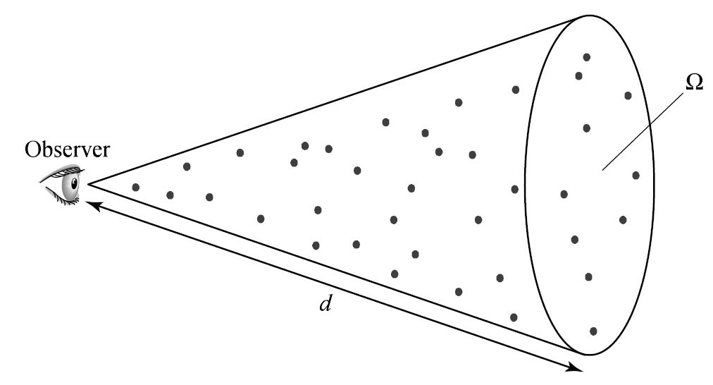
Fig. 5.3 An observer on Earth counting the number of stars within a specified range of spectral and luminosity types out to a distance \(d\) located within a cone of solid angle \(\Omega\). Image Credit: Carroll & Ostlie (2007).#
Let \(n_M(M,\ S,\ \Omega,\ r)dM\) be the number density of stars with absolute magnitudes between \(M\) and \(M+dM\) and attribute \(S\) (e.g., the Morgan-Keenan spectral class) that lie within a solid angle \(\Omega\) in a specific direction at a distance \(r\) from the observer. The number density \(n_M\) has units of \(1/\rm pc^3/mag\), and the actual number density of stars having attribute \(S\) is given by
In Kapteyn’s original study, he considered general star counts that tracked absolute magnitude, regardless of spectral class.
If the number density \(n_M\) is integrated over the volume of a cone defined by the solid angle \(\Omega\) and extending from the observer at \(r=0\) to some distance \(r=d\), the result is \(N_M(M,\ S,\ \Omega,\ d)dM\), which is the total number of stars with absolute magnitudes in the range \(M\) to \(M+dM\) that are found within the conical volume of space. Using \(dV = \Omega r^2 dr\) in spherical coordinates, this is
Equation (5.3) is the general expression for the integrated stars count, written in terms of the limiting distance \(d\). This means that \(n_M dM\) can be obtained from \(N_M dM\) (with limiting distance \(r\)) by differentiating:
Those stars sharing the same absolute magnitude will have different apparent magnitudes because they lie at different distances from us. We can use the distance modulus (corrected for interstellar extinction) to replace the limiting distance \(d\) with the apparent magnitude \(m\). This results in \(\overline{N}_M(M,\ S,\ \Omega,\ m)dM\), which is the integrated star count written in terms of the limiting magnitude or the number of stars that appear brighter than the limiting magnitude \(m\).
If the limiting magnitude is increased slightly, then the limiting distance becomes correspondingly greater and the conical volume is extended to include more stars. The increase in the number of included stars is
This defines the differential star count,
which is the number of stars with an absolute magnitude in the range \(M\) and \(M+dM\) that are found within a solid angle \(\Omega\) and have apparent magnitudes in therange between \(m\) and \(m+dm\).
A simple (and unrealistic) illustration of the use of integrated and differential star counts, consider the case of an infinite universe of uniform stellar density (i.e., \(n_M(M,\ S,\ \Omega,\ r) = n_M(M,S) = \text{constant}\)) and no interstellar extinction (\(A = 0\)). Then Eq. (5.3) becomes (after canceling \(dM\)),
Note
When the last expression is considered over all directions, \(\Omega = 4\pi\) and \(\Omega d^3/3\) is just the volume of sphere of radius \(d\).
Expressing \(d\) in units of parsec and writing it in terms of the apparent magnitude \(m\), we have
Using properties of logarithms, we get (NEED TO CHECK)
If either \(\overline{N}_M\) or \(A_M\) is known from observations, these equations can be used to determine the spatial number density \(n_M(M,\ S)\ dM\).
The constant-density model (described above) suffers from a flaw because the result diverges exponentially as \(m\) increases. This arises when it is used to calculate the amount of light received at Earth due to the stars contained in the solid angle \(\Omega\). This implies an infinite amount of light arriving from infinitely far away!
This dilemma is one expression of Olbers’ paradox, which is a problem known since the time of Kepler and brought to the attention of the general public by Heinrich Olbers about a century later. Restricting ourselves to the Milky Way, the solution rests in its finite size and nonconstant stellar number density. However, the resolution of Olbers’ paradox in not as simple when applied to the universe as a whole.
The modern process of gathering star counts involves the automated use of CCD detectors to determine \(\overline{N}_M\) or \(A_M\). Traditionally, these data are combined with stellar number densities in the Solar neighborhood to estimate the stellar number density for a given spectral type in other regions of the Galaxy.
An iterative computer model would use observations of other galaxies believed to be similar to the Milky Way would compare through successive iterations: the density function, amount of interstellar extinction, and variations in composition with position until a satisfactory match to the original data is obtained. Presumably, this type of model is ideal for applications for Artificial Intelligence (AI) algorithms due to its iterative approach.
5.2. Basic Morphology#
5.2.1. The Distance to the Galactic Center#
Herschel and Kapteyn believed that the Milky Way is possesses a disk of stars including the Sun as a member. Shapley suspected that the Sun does not reside at the center of the disk, but is actually located roughly 1/3 of the way out from the middle. From the Earth, the center of the disk lies in the constellation Sagittarius, corresponding to avery compact emission source known as Sgr \(A^\star\) (A-star) at the J2000 equatorial coordinates
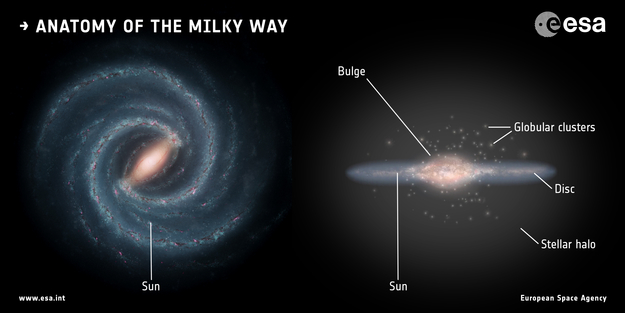
Fig. 5.4 An artist’s depiction of the Milky Way Galaxy seen face-on (left) and edge-on (right) produced by the ESA. Image Credit: Left: NASA/JPL-Caltech; right: ESA; layout: ESA/ATG medialab.#
The Sun’s distance from the center of the Galaxy is known as the solar Galactocentric distance \(R_o\). This value has been revised downward many times since Shapley’s first estimate of \(15\ \rm kpc\), where the modern estimate is \(R_o = 8.5\ \rm kpc\) and is standardized (i.e., uncertainty removed) for the purpose to allow direct comparisons among Galactic structure. However, a number of studies found that \(R_o \simeq 8\ \rm kpc\). In 2003, Eisenhauer et al. (2003) measured \(R_o = 7.94 \pm 0.42\ \rm kpc\) based on astrometric and spectroscopic measurements of \(S2\) (i.e., the closes star to the Galactic center). One of the recent measurements (Abuter et al. (2019)) finds \(R_o = 8.178 (\pm 0.013_{\rm stat} \pm 0.022_{\rm sys})\ \rm kpc\). Carroll & Ostlie (2007) adopted a value of \(R_o = 8\ \rm kpc\) for simplicity, which actually withstands the test of time.
The full diameter of the disk (including the dust, gas, and stars) is believed to be roughly \(50\ \rm kpc\), with estimates ranging from \(40-50\ \rm kpc\). It appears that the disk may not be completely cylindrically symmetric. Rather, the disk may be somewhat elliptical with a ratio of the lengths of the minor and major axes of about 0.9. The solar circle is defined to be a perfect circle of radius \(R_o\).
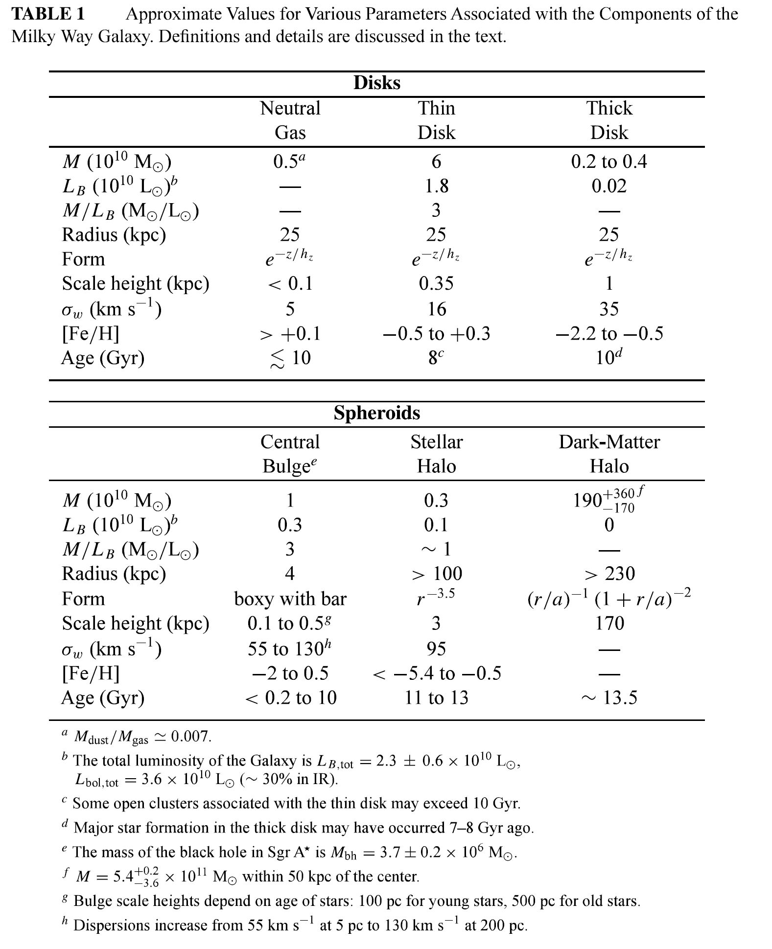
Fig. 5.5 Table of properties of the Milky Way, considering both the disks and spheroids. Image Credit: Carroll & Ostlie (2007).#
5.2.2. The Structure of the Thin and Thick Disks#
The disk is composed of two major components: the thin disk and thick disk.
The thin disk contains relatively young stars, dust, and gas with a vertical scale height of \(\z_{\rm thin} \simeq 350\ \rm pc\) and is region of current star formation. A portion of the thin disk (or sometimes young thin disk) also corresponds to the central plane of the Galactic dust and gas distribution, where it has a scale height of \({\sim}90\ \rm pc\); some have found a scale height as \(35\ \rm pc\).
Note
Recall that one scale height is the distance in which the number density decreases by \(1/e\).
The thick disk probably contains an older population of stars and has a scale height of \({\sim}1\ \rm kpc\). The number of stars per unit volume in the thick disk is only about \(8.5\%\) of that in the thin disk at the Galactic midplane.
When the thin and thick disks are combined, empirical fits to the stellar number density derived from star count data give
where \(z\) is the vertical height above the midplane of the Galaxy, \(R\) is the radial distance (in cylindrical coordinates) from the Galactic center, \(h_R > 2.25\ \rm kpc\) is the disk scale length, and \(n_o \sim 0.02\ {\rm stars/pc^3}\) for the absolute magnitude range \(4.5 \leq M_V \leq 9.5\). Relative to the density coefficient: the scale heights and the disk scale length are all somewhat uncertain. The Sun is a member of the thin disk and is currently located about \(30\ \rm pc\) above the midplane.
The luminosity density (i.e., luminosity per unit volume) of the thin disk is often modeled with the functional form
where \(\text{sech}\) is the hyperbolic secant function. For the thin disk: \(z_o = 2z_{\rm thin}\) and \(L_o \simeq 0.05\ {\rm L_\odot/pc^3}\).
5.2.3. The Age-Metallicity Relation#
The thin and thick disks are further distinguished by the chemical compositions and kinematic properties of their members. Stars are generally classified according to the relative abundance of heavier elements:
Population I stars are metal-rich, with \(Z\sim 0.02\),
Population II stars are metal-poor, with \(Z\sim 0.001\), and
Population III stars are essentially devoid of metals, with \(Z \sim 0\).
In reality, a wide range of metallicities exists in stars. At one end are the extreme Pop. I stars and on the other, the hypothetical Pop. III stars. Between Pop. I and Pop. II stars are intermediate (or disk) population stars.
The important parameter of composition is quantified by the ratio of iron to hydrogen and has become almost universally adopted because iron lines are generally identifiable in stellar spectra. During a supernova detonation (particularly of Type Ia), iron is ejected, which enriches the ISM. New stars can then be created with a greater abundance of iron in their atmospheres relative to their predecessors.
As a result, the iron content should correlate with stellar age, where the youngest (most recently formed) stars have the highest relative abundance of iron. The iron-to-hydrogen ratio in the atmosphere of a star is compared with the Sun’s value through
and is referred to as the metallicity.
Stars with abundances identical to the Sun have \([{\rm Fe}/{\rm H}] = 0.0\), where less metal-rich stars have negative values, and more metal-rich stars have positive values. Measurements of our Galaxy have found values ranging from \(-5.4\) for old, metal-poor* stars to \(0.6\) for young, metal-rich stars.
According to studies of the main-sequence turnoff points in clusters, metal-rich stars tend to be younger than metal-poor stars of a similar spectral type. The apparent correlation between age and composition is called the age-metallicity relation.
in many situations, the correlation between the age and \([{\rm Fe}/{\rm H}]\) may not be as reliable. For example, significant numbers of Type Ia supernovae do not appear until \({\sim}10^9\ \rm yr\) after star formation begins. Since Type Ia are responsible for most of the iron production, iron is not available in large quantities to enrich the ISM.
Mixing of the ISM may after a SN Ia event may not be complete. In other words, a local region of the ISM may become iron-enriched after \(10^9\ \rm yr\), while another region may not experience the same level of enrichment. According to the age-metallicity relation, the iron-rich regin would subsequently produce stars that appear younger, when in fact both regions are the same age.
A second measure of ISM enrichment (and age) is based on \([{\rm O}/{\rm H}]\). Since core-collapse supernova appear after only \(10^7\ \rm yr\) after the onset of star formation and they produce a higher abundance of oxygen to iron, \([{\rm O}/{\rm H}]\) may also be used to determine ages of Galactic components; some astronomers use \([{\rm O}/{\rm Fe}]\) for the same purpose.
5.2.4. Age Estimates of the Thin and Thick Disks#
Typical values for the iron-hydrogen metallicity ratio are:
\(-0.5 < [{\rm Fe}/{\rm H}] < +0.3\) for the thin disk,
\(-0.6 < [{\rm Fe}/{\rm H}] <-0.4\) for the thick disk,
although some thick disk members may have metallicities at least as low as \([{\rm Fe}/{\rm H}] \sim -1.6\).
According to various age determinations, the stellar members of the thin disk are probably significantly younger than their thick-disk counterparts. It appears that star formation began in the thin disk about \(8\ \rm Gyr\) ago and is ongoing today. This conclusion is supported by the observations of white-dwarf stars in the thin disk and theoretical estimates of their cooling times.
There is also evidence that star formation in the thin disk may not have been continuous over time, but actually come in bursts with intervening gaps of several billion years. On the other hand, star formation in the thick disk appears to have predated the onset of star formation in the thin disk by \(2-3\ \rm Gyr\). It is generally believed that the episode of thick-disk star formation spanned the time interval between \(10-11\ \rm Gyr\) ago.
5.2.5. Mass-to-Light Ratios#
From star counts and orbital motions, te estimated stellar mass of the thin disk is roughly \(6\times 10^{10}\ M_\odot\) with another \(0.5 \times 10^{10}\ M_\odot\) of gas and dust. The luminosity in the blue is \(L_B = 1.8 \times 10^{10}\ L_\odot\). When the first of these parameters is divided by the second, the result is the mass-to-light ratio, which is \(M/L_B \approx 3 M_\odot/L_\odot\). This quantity gives us information about the kinds of stars responsible for the generation of the light.
Along the main sequence, a star’s luminosity depends on its mass (i.e., mass-luminosity relation), with
where \(\alpha \simeq 4\) above about \(0.5\ M_\odot\) and \(\alpha \simeq 2.3\) for less massive stars. Assuming that most of the disk stars are on the main-sequence, an “average” stellar mass can be estimated. Substituting the observed mass-to-light ratio and solving for the mass, we have
Assuming that \(\alpha \simeq 4\), we find that \(\langle M \rangle \simeq 0.7\ M_\odot\). Apparently the total luminosity of the disk is dominated by stars somewhat less massive than the Sun. This should not be surprising since the initial mass function (IMF) indicates that many more low-mass than high-mass stars are created out of the interstellar medium. This is also consistent with M-dwarf stars being the most common class of stars in the Sun’s vicinity.
The \(B\)-band luminosity of the thick disk is \(2\times 10^8\ \rm L_\odot\), or \(1\%\) of the thin disk’s luminosity. This explains why the thick disk is so difficult to detect. The mass of the thick disk is probably about \(2-4 \times 10^9\ M_\odot\), or approximately \(3\%\) of the thin-disk mass.
5.3. The Structure of the Milky Way Galaxy#
5.3.1. Spiral Structure#
Significant structure exists within the disk. Neutral hydrogen clouds, relatively young objects (e.g., O and B stars), H II region, and galactic (open) clusters are used as tracers of Galactic structure. From these tracers, a spiral structure emerges, which gives the disk the appearance of a pinwheel. When other galaxies (with distinct disks) are observed in blue light, these galaxies often exhibit similarly beautiful spiral structure (e.g., the great spiral galaxy of Andromeda).

Fig. 5.6 The Andromeda Galaxy (aka M31 or NGC 224) is a spiral galaxy believed to be much like our own. Image Credit: Wikipedia:Andromeda Galaxy.#
However, when the galaxies are viewed in red light, which is characteristic of older, low-mass stars, the spiral structure is less pronounced. It appears that spirals are associated with ongoing star formation and that older stars have had ample time to drift out of the spiral pattern. The Sun seems to be located close to (but not actually in) one of the spiral arm features known as the Orion-Cygnus arm, or the Orion spur since it is probably not a full spiral arm structure. Spiral arms get their names from the constellations in which they are observed.
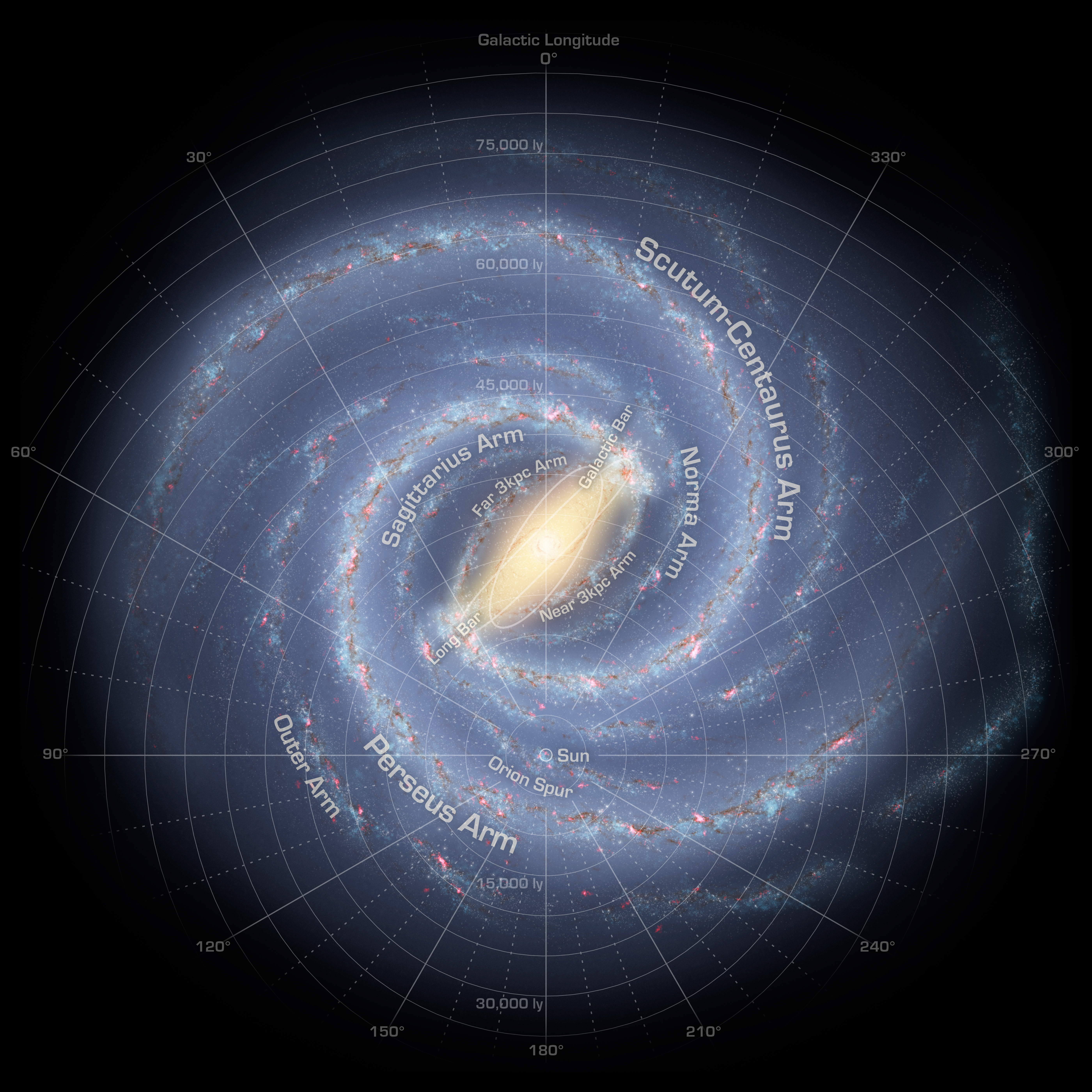
Fig. 5.7 Artist’s concept of the Milky Way, which illustrates the structure of the spiral arms. Image Credit: NASA/JPL-Caltech/R. Hurt (SSC/Caltech).#
The interstellar gas and dust clouds are clearly evident, located near the midplane, and found preferentially in the spiral arms. If it were possible to view our Galaxy from a exterior vantage point (outside the disk but along the plane), it would probably appear similar to NGC 891.

Fig. 5.8 NGC 891 seen edge-on, which clearly shows a thin dust band in the plane of the disk. Image Credit: Adam Block; Mt. Lemmon Sky Center; U. Arizona.#
5.3.2. Interstellar Gas and Dust#
Gas and dust clouds exist in the Milky Way with a range of masses, temperatures, and densities. From these clouds, new stars are ultimately formed. Astronomers have mapped out the overall distribution of dust and gas within the Milky Way by measuring the effects of obscuration by (and emissivity of) dust, as well as the location of the 21-cm H I emission, and the \(\rm CO\) molecule as a tracer of \(\rm H_2\).
Molecular hydrogen \(\rm H_2\) and cool dust are found predominantly between \(3-8\ \rm kpc\) and \(3-7\ \rm kpc\) from the Galactic center, respectively (i.e., inside the solar circle), while the atomic hydrogen \(\rm H\) can be found from \(3\ \rm kpc\) out to the edge of the Galactic disk (\(25\ \rm kpc\)). It appears that \(\rm H_2\) and the dust are more tightly confined to the Galactic plane, with vertical scale heights above or below the midplane of \(\lesssim 90\ \rm pc\). This is only about \(25\%\) of the value for stars in the thin disk and on the order of \(9\%\) of the scale height of thick-disk stars.
In the region near the Sun, the scale height for atomic hydrogen is approximately \(160\ \rm pc\). The total mass of H I is estimated to be \(3\times 10^9\ M_\odot\), and the mass of \(\rm H_2\) is \({\sim}10^9\ M_\odot\). In the solar neighborhood, the total mass density of gas is \(0.04\ M_\odot/{\rm pc^3}\), where hydrogen accounts for approximately \(77\%\) of it, molecules contribute \(17\%\), and ions add an additional \(6\%\).
At distances beyond \(12\ \rm kpc\) from the Galactic center, the scale heigh of H I increases dramatically, extending up to \(900\ \rm pc\). In addition, the distribution of H I in the outer reaches of the Galaxy is no longer strictly confined to the plane, but exhibits a well-defined warp that reaches a maximum deviation angle from the plane of \(15^\circ\).
Warped H I distributions (e.g., the one observed in our own Galaxy) appear to be common features in other spiral galaxies, including Andromeda, and in some spiral galaxies the warp angle can reach \(90^\circ\). Warps do not seem to the result of simple gravitational perturbations from one or more external galaxies, but they do seem to associated with the distribution of mass in the outer regions of the Galaxy (beyond where most of the luminosity is produced).
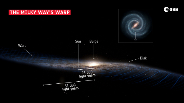
Fig. 5.9 The structure of our galaxy with its warped galactic disk produced by the ESA. Image Credit: Stefan Payne-Wardenaar; Inset: NASA/JPL-Caltech; Layout: ESA.#
Hydrogen clouds can be found at high latitudes. Although some of these clouds have positive radial velocities (implying that they are moving away from the disk), the majority possess large negative radial velocities (up to \(400\ \rm km/s\) or more), as measured by their 21-cm emission. There appear to be two types of sources responsible for these high-velocity clouds.
Galactic fountain model: Clouds of gas ejected from supernovae are driven to large values of \(z\), where they eventually cool and rain back down onto the Galactic plane.
It also appears that the Galaxy is accreting gas from intergalactic space and from its small satellite galaxies, which explains the predominance of negative radial velocity clouds.
Coronal gas: A very hot, tenuous gas exists at distances up to or exceeding \(70 \rm kpc\) from the Galactic center.
The Far Ultraviolet Spectroscopic Explorer (FUSE) has detected \(\rm O\ VI\) absorption lines in the spectra of distant extragalactic sources and halo stars produced when the light passes through the gas in the Galactic halo.
Using \(\rm O\ VI\) as a tracer of the hydrogen gas, the strengths of \(\rm O\ VI\) absorption lines imply a number density of hydrogen \(n_H \sim 10^{-11}\ \rm m^{-3}\).
Assuming that the distribution is approximately spherical with a radius of \(R\sim 70\ \rm kpc\) leads to an estimate for the mass of the gas \(M_{\rm gas} \simeq 4 \times 10^8\ M_\odot\).
To support the gas against gravitational collapse, the gas temperature must be very hot. It is estimated to be in excess of \(10^6\ \rm K\) (similar to the Sun’s corona), with the high gas temperature perhaps being due to collisions between infalling gas and existing gas in the Galaxy.
5.3.3. The Disruption of Satellite Galaxies#
The Magellanic Stream is a narrow band of H I emission stretching \(>180^\circ\) across the sky and trailing the Magellanic Clouds of the Souther Hemisphere. The Magellanic Stream appears to be the result of a tidal encounter of the Magellanic Clouds with the Milky Way some \(200\ \rm Myr\) ago.
Other satellite galaxies have also tidally interacted with the Milky Way. For example, Ibata et al. (1995) announced the discovery of a previously unknown dwarf spheroidal galaxy in Sagittarius. At a distance of only \(24\ \rm kpc\) from Earth and \(16\ \rm kpc\) from the center of the Milky Way, the Sagittarius dwarf spheroidal is the closest galaxy to Earth. It is elongated with the long axis directed toward the Galactic center and has underwent only a few orbital encounters (with a radial velocity of \(140\ \rm km/s\)) with the Milky Way. Evidently the Sagittarius dwarf spheroidal galaxy (along with its globular clusters) is being incorporated into the Milky Way.
Using the 2-Micron All Sky Survey (2MASS) catalog, researchers have identified an overdensity of stars in the Canis Major near the plane of the Milky Way. A group of globular and open clusters are associated with this overdensity in both position and radial velocity. This suggests that another dwarf satellite galaxy was integrated into the Milky Way in the past and may now be a part of the thick disk.
The unusual globular cluster, \(\omega\) Centuari, also seems to be the remnant of a dwarf galaxy that has been subsumed by the Milky Way. \(\omega\) Cen is the largest and brightest globular cluster visible from Earth and has an unusually high surface brightness. It appears that this globular cluster is the stripped core of another former satellite galaxy.
5.3.4. The Galactic Bulge#
Although the vertical scale height of the thin disk is near \(350\ \rm pc\) in the Sun’s vicinity, the scale height increases somewhat toward the inner regions of the Galaxy, where the disk meets the Galactic bulge. The bulge is not simply an extension of the disk but is an independent component of the Galaxy. The mass of the bulge is roughly \(10^{10}\ M_\odot\) and its \(B\)-band luminosity is near \(3\times 10^9\ L_\odot\). This gives a mass-to-light ratio of \(3\ M_\odot/L_\odot\), which is comparable to the mass-to-light ratio for the thin disk.
The boxy (or elongated) bulge is evident in the COsmic Background Explorer (COBE) satellite image of the Galaxy. The image was produced by combining observations at \(1.2,\ 2.2,\ \text{and } 3.4\ \rm \mu m\). Using the COBE data together with observations of RR Lyraes and cool (K and M) giants, we find that the variation in the number density of stars in the bulge corresponds to a vertical scale height from \(100-500\ \rm pc\), depending on the stellar ages used to make the determination (i.e., younger stars yield smaller scale heights).
The surface brightness \(I\) of the bulge (measured in units of \(L_\odot/{\rm pc}^2\)) exhibits an approximate radial dependence of the form
which is a \(r^{1/4}\) law (or de Vaucoulurs profile) described by the effective radius \(r_e\) and the surface brightness \(I_e\) measured at \(r_e\). Formally, \(r_e\) is the radius in which 1/2 of the bulge’s light is emitted. At the infrared wavelength of \(12\ \rm \mu m\), star count data from the InfraRed Astronomical Satellite (IRAS) suggests an effective radius of \({\sim}0.7\ \rm kpc\). Similar results were found by COBE.
A serious difficulty in observing the properties of the bulge rests in the large amount of extinction at visible wavelengths due to the dust between the Sun and the Galactic center. The total amount of extinction within several degrees of the center can be more than \(30\ \rm mag\). However, a number of lines of sight exist for which the amount of extinction is minimal.
The most well-known of these is Baade’s window, which Walter Baade discovered in 1944 while observing the globular cluster NGC 6522. Baade realized that by observing in that region of the sky, he was able to see RR Lyraes that were actually beyond the Galactic center. Baade’s window is \(3.9^\circ\) below the Galactic center, and the line of sight passes within \(550\ \rm pc\) of the center.
From the observational evidence, the chemical abundances of stars in the bulge vary significantly, ranging from quite metal-poor to very metal-rich (\(-2< \left[{\rm Fe}/{\rm H}\right] <0.5\)). Based on chemical abundances, it appears that three somewhat distinct age groupings in the central bulge.
very young, with ages less than \(200\ \rm Myr\),
ages between \(200\ {\rm Myr}\) and \(7\ \rm Gyr\), and
older than \(7\ \rm Gyr\) (perhaps up to \(10\ \rm Gyr\) or older).
In a trend that seems counterintuitive, the oldest stars in the bulge tend to have the highest metallicities across the range from \(-2\) to \(0.5\). This is probably due to a burst of massive star formation when the Galaxy was young. Apparently core-collapse supernovae enriched the ISM early in the life of the bulge, which implies that subsequent generations of stars contained an enhanced abundance of heavier elements. The more uniform distribution of metallicity in recent generations of stars could be the result of fresh, infalling material.
5.3.5. The Milky Way’s Central Bar#
Although it was originally thought to be essentially spheroidal in nature, a number of observing campaigns and database studies have determined that the bulge contains a distinct bar. The Milky Way’s central bar has a radius (i.e., half-length) from the Galactic center of \(4.4\pm 0.5\ \rm kpc\) and is oriented at an angle \(\phi = 44^\circ \pm 10^\circ\) with respect to the line-of-sight angle from Earth to the Galactic center. It seems tha the bar is somewhat thicker in the plane of the Galaxy than in the \(z\) direction.
5.3.6. The 3-kpc Expanding Arm#
In the inner regions of the Galaxy, a unique feature is most easily observed at the 21-cm wavelength of H I, which is the 3-kpc expanding arm. It is a gas cloud that is moving toward us at \({\sim}50\ \rm km/s\).
Once believed to be the product of a gigantic explosion in the center of the Galaxy, the rapidly moving structure is now thought to be a consequence of the presence of the stellar bar. Rather than being driven away from the center in an explosive event that would require and unrealistic \(10^{52}\ \rm J\) of energy, the gas cloud is merely in a very elliptical orbit about the Galactic center resulting from gravitational perturbations from the bar.
5.3.7. The Stellar Halo and Globular Cluster System#
The last luminous component of the Galaxy is the stellar halo, which is composed of the globular clusters and high velocity (perpendicular to the Galactic plane) field stars. These field stars are called high-velocity stars, since their velocity components differ significantly compared to the Sun. Most of the globular clusters and the high-velocity stars can reach positions that are far above or below the plane of the Galaxy.
It appeared to Shapley, that all of the known globular clusters were distributed nearly spherically about the Galactic center, but it has become apparent that two distinct spatial distributions exist (delineated by metallicity).
Older, metal-poor clusters whose members have \([{\rm Fe}/{\rm H}] < -0.8\) belong to an extended spherical halo of stars,
young clusters with \([{\rm Fe}/{\rm H}] > -0.8\) form a much flatter distribution and may even be associated with the thick disk.
The notable exception is the well-studied globular cluster 47 Tucana (47 Tuc or NGC 104), which is located \(3.2\ \rm kpc\) below the Galactic plane and has an unusually high metallicity of \([{\rm Fe}/{\rm H}] = -0.67\). Some astronomers have argued that 47 Tuc is a member of the halo population, while others consider 47 Tuc to be a member of the thick disk.
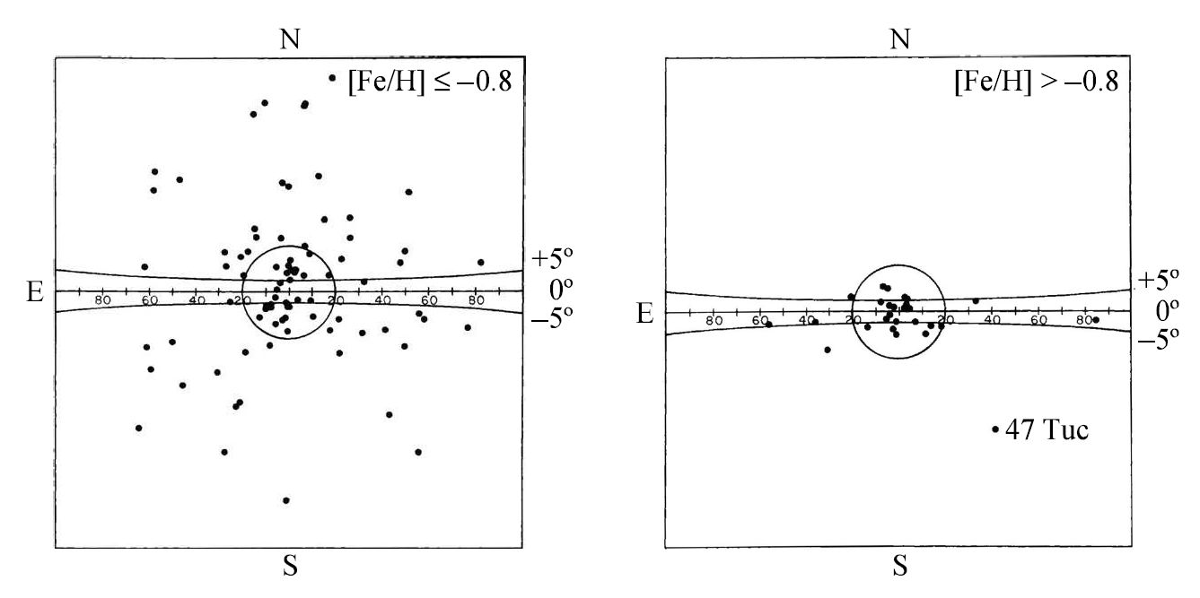
Fig. 5.10 Metal-poor globular clusters form a nearly spherical distribution about the Galactic center, while more metal-rich clusters are found near the Galactic plane. Image Credit: Carroll & Ostlie (2007). Figure adapted from Zinn (1985).#
Our Galaxy is known to contain at least 150 globular clusters with distances from the Milky Way ranging from \(0.5-120\ \rm kpc\). The youngest globular clusters appear to be about \(11\ \rm Gyr\) old, and the oldest are probably a little over \(13\ \rm Gyr\) old (nearly the age of the universe; see Krauss & Chaboyer (2003)). It now appears that a significant age spread of 2 billion years or so exists between the youngest and oldest members of the halo.
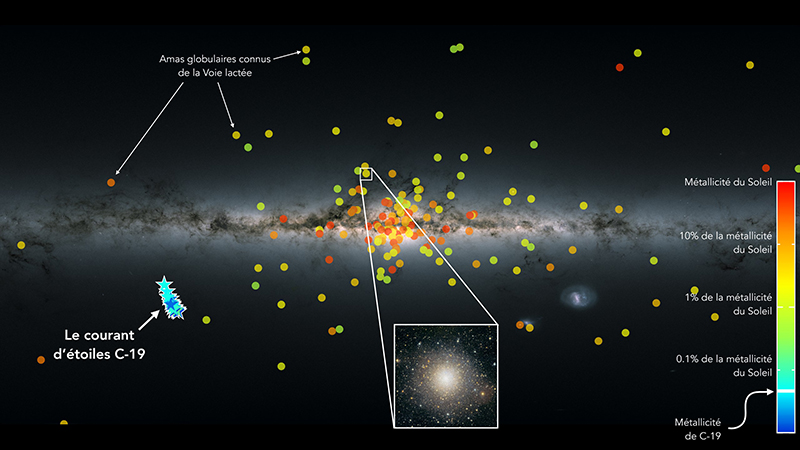
Fig. 5.11 Distribution of globular clusters in the Milky Way superimposed on a map of the Milky Way compiled from data obtained with the Gaia Space Observatory. Figure Credit: CNRS. Image Credit: N. Martin / Strasbourg Astronomical Observatory / CNRS; Canada-France-Hawaii Telescope / Coelum; ESA / Gaia / DPAC.#
Although 144 of the globular clusters are found within \(42\ \rm kpc\) of the Galactic center, 6 globular clusters have been found between \(69-123\ \rm kpc\) of the Galactic center. Some astronomers have suggested that those six most distant clusters may have been captured by the Milky Way or may be dwarf spheroidal galaxies, much as \(\omega\) Cen and the Sagittarius dwarf galaxy may have been. If we do not include these very remote objects, the metal-poor clusters seem to be confined to a halo with a radius of \({\sim}42\ \rm kpc\). The detection of extremely distant and luminous field stars suggests that a stellar halo radius of \(50\ \rm kpc\) could be more appropriate.
The number density profile of the metal-poor globular clusters and the field stars has the form
where \(n_{o,\rm halo} \simeq 4 \times 10^{-5}\ {\rm pc^{-3}}\) is roughly \(0.2\%\) of the thin disk’s midplane. The scale length \(a\) of the number density distribution is several thousand parsecs. At visible wavelengths, the effective radius of the halo \(r^{1/4}\) law is \(r_e = 2.7\ \rm kpc\).
5.3.8. The Dark Matter Halo#
When the masses of all the luminous components of the Galaxy are combined (e.g., thin and thick disks, ISM, Galactic bulge, stellar halo, and the bar), the total mass of luminous matter in the Galaxy is estimated to be \(9 \times 10^{10}\ M_\odot\). There is another crucial component to the overall structure of our Galaxy. There may also be an unseen element that is responsible for the generation of the warps in the H I distribution near the outer edges of the luminous disk.
This dark matter halo seems to be roughly spherically distributed, enveloping the stellar halo and extending out to \({\sim}230\ \rm kpc\). The dark matter halo has an apparent mass distribution of the form,
where \(\rho_o\) and \(a\) are fitted coefficients using the mass distribution in the dark matter halo.
This functional dependence behaves as \(1/r\) when \(r\ll a\) and as \(1/r^3\) when \(r\gg a\). The mass of the dark matter halo can be \(5.4 \times 10^{11}\ M_\odot\) and \(1.9 \times 10^{12}\ M_\odot\) within \(50\ \rm kpc\) or \(230\ \rm kpc\) of the Galactic center, respectively. It appears that the dark matter halo accounts for about \(95\%\) of the entire mass of the Galaxy.
The composition of the dark matter halo is still under investigation. Some sources of mass have been excluded, where it cannot be interstellar dust because the dust block starlight and allow us to detect its presence. The dark matter halo cannot be composed of gas, because absorption lines would be apparent when observing halo stars.
One possible set of candidates are weakly interacting massive particles (WIMPs). The WIMPs would not contribute to the overall luminosity of the Galaxy, but they would affect it through their gravitational interactions. In support of a WIMP-dominated Galaxy, theoretical calculations of the formation and evolution of the universe suggest that non-baryonic matter (i.e., constituents of matter that are not protons, neutrons and related massive particles) may constitute the majority of the mass for the dark matter halo.
A competing hypothesis suggests that massive compact halo objects (MACHOs) may be responsible. MACHOs that could supply the unseen mass could be white dwarfs, neutron stars, black holes, or less exotic red or brown dwarfs. Some searches for MACHOs are based on the general relativistic prediction that starlight is deflected as it passes near a massive object. If a MACHO is located between a distant star and Earth, the light from the star can be focused with the MACHO acting as a gravitational lens.
5.3.9. The Galactic Magnetic Field#
The Galaxy possess a magnetic field. The orientation and strength of the field can be measured using the Zeeman effect and the polarization of visible- and radio-wavelength electromagnetic radiation by reflection from interstellar grains aligned with the field. It appears that within the disk , the field tends to follow the Galaxy’s spiral arms and has a typical strength of \(0.4\ \rm nT\). The field strength near the Galactic center may reach \(1\ \mu T\).
The global Galactic magnetic field is quite weak relative the Earth’s magnetic field near the surface (\({\sim}50\ \mu T\)), but it likely plays a role in the structure and evolution of the Milky Way. The energy density within the Galaxy appears to be comparable to the thermal energy density of gas within the disk.
5.4. The Kinematics of the Milky Way#
5.4.1. The Galactic Coordinate System#
The Galactic midplane is not aligned with the plane of the celestial equator but is inclined at an angle of \(62.87^\circ\). As a result, rather than using the Earth-based equatorial coordinate system, it is more convenient to introduce a new coordinate system when discussing the structure and kinematics of the Galaxy. The Galactic coordinate system exploits the natural symmetry introduced by the existence of the Galactic disk.
The intersection of the midplane of the Galaxy with the celestial sphere forms what is very nearly a great circle (i.e., Galactic equator). The Galactic latitude (\(b\)) and longitude (\(\ell\)) are defined from a vantage point to be the Sun. Galactic latitude is measured in degrees north or south of the Galactic equator along a great circle that passed through the north Galactic pole. Galactic longitude (in degrees) is measured east along the Galactic equator (near the Galactic center) to the point of intersection with the great circle used to measure the Galactic latitude.
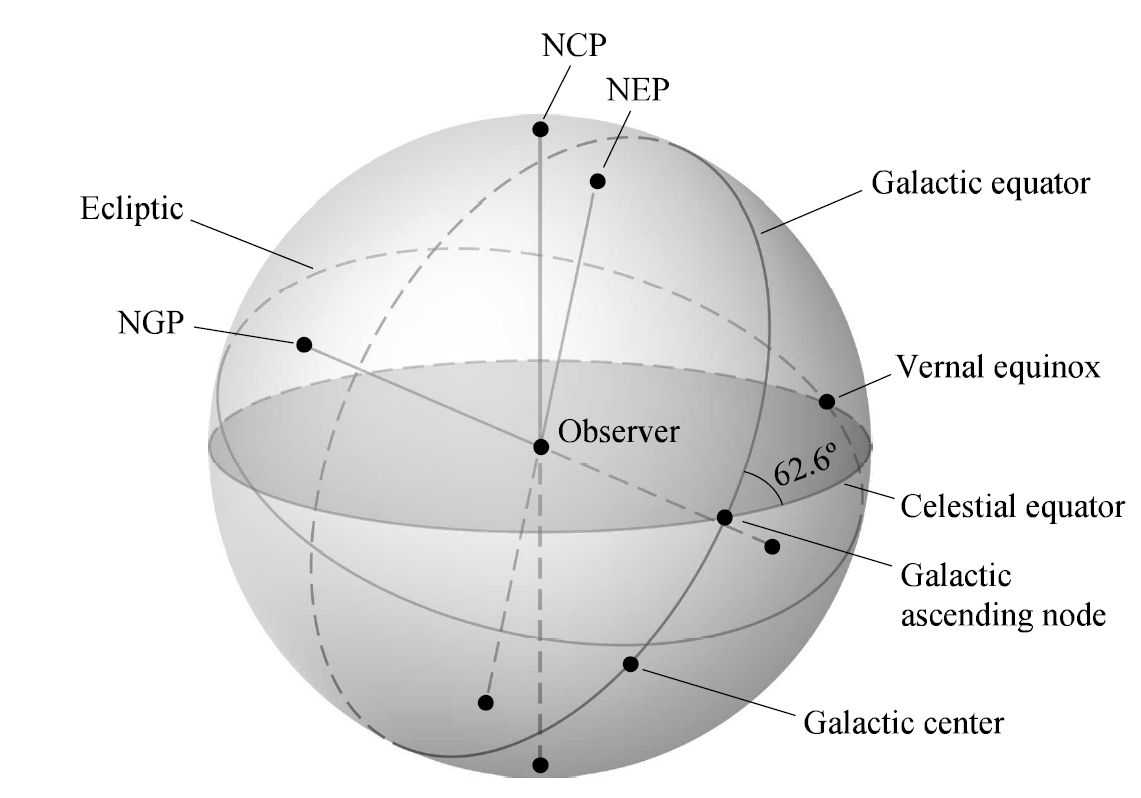
Fig. 5.12 The relative orientations of the celestial equator, ecliptic, and Galactic equator on the celestial sphere. Image Credit: Carroll & Ostlie (2007).#
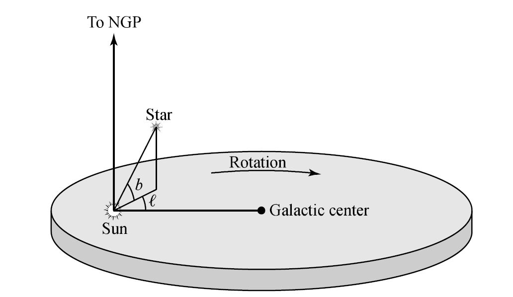
Fig. 5.13 The definition of the Galactic coordinates \(\ell\) and \(b\), where the Galactic rotation is clockwise about the Galactic center. Image Credit: Carroll & Ostlie (2007).#
By international convention, the J2000 equatorial coordinates of the north Galactic pole (\(b=90^\circ\)) and the origin of the Galactic coordinate system (\(\ell_o = 0^\circ,\) \(b_o = 0^\circ\)) are
Note
The center of the Galaxy \((\alpha_{\rm Sgr\ A^\star},\ \delta_{\rm Sgr\ A^\star})\) is very close to, but not exactly aligned with \((\ell_o = 0^\circ,\ b_o=0^\circ)\)
Two other useful positions on the sky are also worth specifying in both coordinate systems. The location of the north celestial pole (\(\delta_{\rm NCP}=90^\circ\)) is given in J2000 Galactic coordinates as
The intersection of the celestial equator with the Galactic equator moving eastward from negative to positive declination (i.e., the ascending node) is given in equatorial coordinates by
The transformation between equatorial to Galactic coordinates involves the following transformations:
or
Note
Calculators may return the wrong quadrant when the calculation of the inverse trigonometric function is performed. Therefore, the ratio between two equations are taken to produce a tangent function and then the arctan2 function is used to ensure that the proper quadrant is used.
The ascending node in equatorial coordinates can be converted into Galactic coordinates to get
import numpy as np

def ra2deg(hh,mm,ss):
    return (hh + mm/60. + ss/3600.)/24. * 360.
def dec2deg(deg,min,sec):
    return deg + min/60.+ sec/3600.

def eq2Gal(alpha,delta):
    sinb = np.sin(delta_NGP)*np.sin(delta) + np.cos(delta_NGP)*np.cos(delta)*np.cos(alpha-alpha_NGP)
    tan_y = np.cos(delta)*np.sin(alpha-alpha_NGP)
    tan_x = np.cos(delta_NGP)*np.sin(delta)-np.sin(delta_NGP)*np.cos(delta)*np.cos(alpha-alpha_NGP)
    return ell_NCP-np.arctan2(tan_y,tan_x), np.arcsin(sinb) #return ell, b


alpha_NGP = np.radians(ra2deg(12,51,26.28))
delta_NGP = np.radians(dec2deg(27,7,41.7))
ell_NCP = np.radians(dec2deg(123,0,0))

alpha = np.radians(ra2deg(18,51,24))
delta = 0.

ell_asc, b_asc = eq2Gal(alpha,delta)
print(np.degrees(ell_asc),np.degrees(b_asc))


from astropy.coordinates import SkyCoord
from astropy import units as u

c = SkyCoord('18h51m24s +00d00m00s', frame='icrs')
print(c.ra.hms, c.dec)
c = c.transform_to('galactic')
print(c.l.deg, c.b.deg)
32.9956681540949 0.008454886823038963
hms_tuple(h=18.0, m=51.0, s=24.000000000021657) 0d00m00s
32.927603488779674 0.0084352132549898
5.4.2. A Cylindrical Coordinate System for Galactic Motions#
The motions of stars in the solar neighborhood allow us to glean important clues regarding the large-scale structure of the Galaxy. The Galactic coordinate system is useful for representing the locations of objects within the Galaxy as seen from Earth, it is not the most convenient choice for studying kinematics and dynamics.
One reason is that the Sun, which is the origin of the Galactic system, is itself moving about the center of the Galaxy. In addition, a coordinate system centered on the Sun constitutes an noninertial reference frame with respect to Galactic motions.
To complement the Galactic coordinate system, a cylindrical coordinate system is used that places the center of the Galaxy at the origin. In this system,
the radial coordinate \(R\) increases outward,
the angular coordinate \(\theta\) is pointed in the direction of rotation of the Galaxy, and
the vertical coordinate \(z\) increases to the north.
The corresponding velocity components are traditionally labeled as
This set of directional choices results in a left-handed coordinate system instead of the more conventional right-handed one. This occurs because, when viewed from the NGP, the Galaxy rotates clockwise, rather than counter-clockwise.
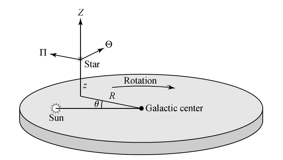
Fig. 5.14 The cylindrical coordinate system to analyze Galactic kinematics. Image Credit: Carroll & Ostlie (2007).#
5.4.3. Peculiar Motions and the Local Standard of Rest (LSR)#
All of our observations are made from Earth, where we can transform those observations to Sun-centered ones by removing any effects resulting from the rotational and orbital motions of Earth. As a result, we can consider the Sun as the site of all observations of the Galaxy. Since the Earth-Sun distance is very small when compared to any distances on a Galactic scale, we only need to deal with changes in velocity and can (mostly) ignore the changes in position.
The Sun does not follow a simple planar orbit (or even a closed non-planar orbit). Instead, it is moving slowly inward (i.e., in the \(-R\) direction) and farther north, away from the midplane (i.e., \(+z\) direction) as it moves about the Galactic center. To investigate the motion of the Sun, we will first define the dynamical local standard of rest (dynamical LSR) to be a point that is instantaneously centered on the Sun and moving in a perfectly circular orbit. along the solar circle about the Galactic center.
Note
An alternative definition for the LSR is known as the kinematic local standard of rest, which is based on the average motions of stars in the solar neighborhood. With the right choice of reference stars, the dynamical and kinematic LSRs agree quite well. But, it can be shown that the kinematic LSR systematically lags behind the dynamical LSR. Carroll & Ostlie (2007) use “the LSR” to refer to the dynamical LSR.
The velocity components of the LSR must be
where \(\Theta_o \equiv \Theta(R_o)\) and \(R_o\) is the solar Galactocentric distance.
Note that once the LSR is chosen, the Sun immediately begins to drift away from it, which implies that twe would effectively need to redefine the reference point constantly. In reality, this is not a significant problem because the \(230\ \rm Myr\) orbital period of the LSR is long compared to the time since modern telescopic observations began. Consequently there has not been sufficient time for the effect to become noticeable.
The velocity of the a star relative to the LSR is known as the star’s peculiar velocity and is given by,
The Sun’s peculiar velocity relative to the LSR is generally referred to as simply the solar motion.
The average of \(u\) and \(w\) for all stars in the solar neighborhood (excluding the Sun) should be nearly zero if we assume an axisymmetric Galaxy. There should be as many stars moving inward as outward, and there should be as many stars moving toward the NGP as toward the SGP due to symmetries about both the rotation axis and the midplane. In reality, this is not quite true because the Galaxy is not precisely axisymmetric, but the error is not that significant.
We assume that summing over a sample of \(N\) nearby stars,
The same assumption cannot be made for the \(v\) component. Consider the orbits of three hypothetical stars \((A,\ B,\ C)\) that intersect at the LSR. Stars with different average orbital radii (as with elliptical orbits) must follow paths that bring them very close to the LSR if they are members of the solar neighborhood and eligible for inclusion in the calculation of \(\langle v \rangle\).
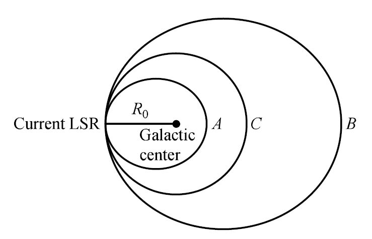
Fig. 5.15 The orbits of three hypothetical stars \((A,\ B\, C)\) intersecting at the LSR. The stars \(A\) and \(B\) have elliptical orbits with semimajor axes \(a_A < R_o\) and \(a_B > R_o\), respectively. The star \(C\) orbits on a circular path coinciding with the LSR. Image Credit: Carroll & Ostlie (2007).#
If we consider the special case that \(u = w = 0\) for all stars in our sample, then the stars must be at either their most distant point (apogacticon) or closest approach (perigalacticon) from the Galactic center when they coincide wth the LSR. Then, for two stars \((A,\ B)\) to follow their specified orbits, it is necessary that \(\Theta_A(R_o) < \Theta_o\) and \(\Theta_B(R_o) > \Theta_o\). This implies that \(v_A <0\) and \(v_b > 0\). Since more stars reside inside the Galactocentric distance than beyond it,
The velocity that is measured for a particular star relative to the Sun is just the difference between the star’s peculiar velocity and the solar motion with respect to the LSR, or
Using the average values of the stellar peculiar velocity components and solving for the solar motion, we have
The \(u\) and \(w\) components of the solar motion simply reflect the averaged relative velocities of the other stars with respect to the Sun in the \(R\) and \(z\) directions. Qualitatively, these stars appear to be “streaming” past the Sun as it moves through space.
To find the \(v\) component of the solar motion, we must first determine the average value of \(v\) for stars in the solar neighborhood. Qualitatively, the procedure involves deriving an analytical expression for \(\langle v \rangle\) in terms of the radial variation in the number density of stars in the solar neighborhood. The justification for this relationship lies in the argument made concerning the lag of stellar motions behind the LSR due to the increase in the number density with decreasing Galactocentric distance.
The result is an equation of the form,
where \(C\) is a constant and
measures the spread in the \(R\) components of the peculiar velocities of stars in the solar neighborhood (with respect to the LSR) and \(\sigma_u^2 = \langle \Pi \rangle\).
Note that \(\sigma_u\) is related to the standard deviation of the velocity distribution, or
In the special case that \(\langle u \rangle = 0\), then \(\sigma_u = \langle u^2 \rangle^{1/2}\) is identical to the standard deviation, where \(\sigma_u \) is known as the velocity dispersion in \(u\).
A stellar sample that produces a larger dispersion in \(u\) means that a wider range of elliptical orbits are included (see elliptical orbit). This results in a more negative average value of \(v\) for the sample because there is a larger fraction of the stellar population with \(R < R_o\). As \(\sigma_u^2\) decreases, fewer stars are appreciably noncircular and \(\langle v \rangle\) will approach zero. The average deviation in velocity can be written (using \(v_\odot\)) as
where \(-v_\odot\) is simply the \(y\) intercept on a graph of \(\langle \Delta v \rangle\) versus \(\sigma_u^2\) and \(C\) is the slope of the line.
The components of the Sun’s peculiar velocity are
so that the Sun is moving (relative to the LSR):
toward the Galactic center,
more rapidly in the direction of the Galactic rotation, and
north out of the Galactic plane.
Overall, the solar motion is \({\sim 13.4\ {\rm km/s}}\) toward a point in the constellation of Hercules. The solar apex is the point in which the Sun is moving toward, where the solar antapex is the point in which the Sun is retreating. The exact value for the solar motion and the location of the solar apex depend on the choice of the reference stars.
With the Sun’s motion known, the velocities of stars relative to the Sun can be transformed into peculiar motions relative to the LSR. This is similar to how the relative motions of the planets were known but not quantified until the actual distance for 1 AU was measured.
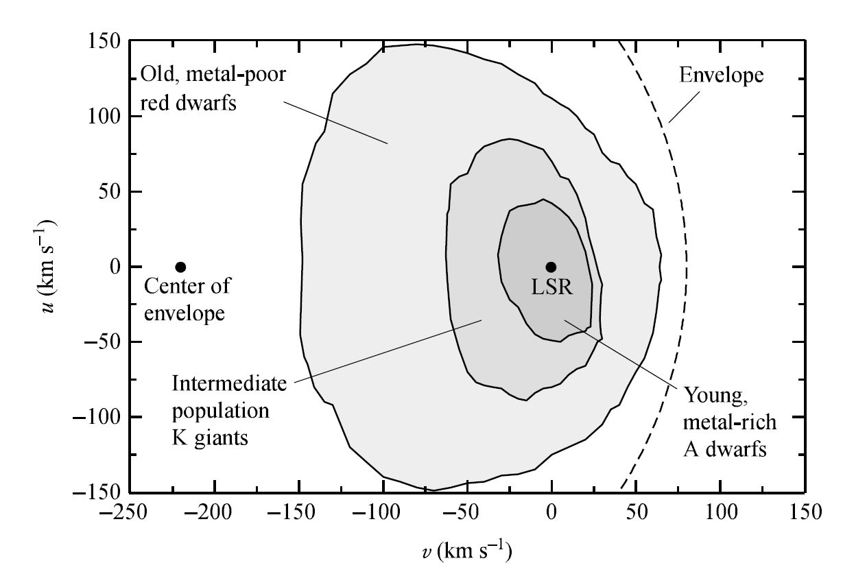
Fig. 5.16 A schematic diagram of the peculiar velocity components \(v\) and \(u\) for stars in the solar neighborhood. The contours represent the metal-rich main sequence A stars (inner), older K giants (middle), and very metal-poor red dwarfs (outer). The LSR lies at the origin \((v,\ u) = (0,\ 0)\), where an enveloping circular contour (\({\sim}300\ {\rm km/s}\) in radius) that is centered at \(v= -220\ \rm km/s\) reveals the orbital velocity of the LSR. Image Credit: Carroll & Ostlie (2007).#
It is then possible to plot the component peculiar motion against another component for a specified sample of stars in the solar neighborhood to obtain important information about their kinematics, where these plots are known as velocity ellipsoids.
Metal-rich main-sequence A stars are used, the range in velocities about the LSR has a small dispersion.
Older K giants show a wider variation in both \(u\) and \(v\).
Old metal-poor red dwarfs illustrate a larger dispersion (spread).
The same is seen in plots of \(w\) versus \(v\), whereas a more symmetric diagram results when \(w\) is plotted against \(u\). There is a noticeable relationship between the metallicity and velocity dispersion, which is called the velocity-metallicity relation. By combining the velocity-metallicity and age-metallicity relations, the velocity ellipsoids suggest that the oldest stars in the Galaxy have the wides range of peculiar velocities.
Because stars with the smallest peculiar velocities don’t drift away from the LSR as quickly, they must occupy orbits that are similar to the LSR and implies that these young stars are members of the thin disk. On the other hand, the stars with the largest peculiar velocities follow very different paths about the center of the Galaxy. In particular, stars with large \(|w|\) must be passing through the solar neighborhood on trajectories that will carry them to great distances above and below the disk. These old, metal-poor stars are the high-velocity stars that are a part of the stellar halo.
A second common feature of peculiar velocity diagrams is the clear asymmetries in the velocity ellipsoids along the \(v\) axis as a function of metallicity or age, where this is known as asymmetric drift. Few stars are observed with \(v > + 65\ \rm km/s\), but there are metal-poor RR Lyraes and subdwarfs with \(v< - 250\ \rm km/s\). A nearly circular “envelope” with a radius of \(300\ \rm km/s\) can be drawn around the high-velocity stars. The center of the velocity envelope appears to be near \(v=-220\ \rm km/s\) for both \(u-v\) and \(w-v\) diagrams.
If on average, the stellar halo is rotating very slowly (if at all), then the orbital velocity of the LSR should reveal itself as a point of symmetry along the \(v\) axis. This is because halo stars with \(\Theta \simeq 0\) (i.e., no motion along the direction of Galactic rotation) should exhibit peculiar velocities that simply reflect the motion of the LSR (i.e., \(v\simeq -\Theta_o\)). Stars that have orbital components that are in the opposite sense from the overall Galactic rotation direction have \(v< -\Theta_o\). Through this argument, the orbital speed of the LSR is given as
and is the presently accepted IAU standard.
Note
Kuijken and Tremaine (1994) suggested that the IAU value of \(\Theta_o\) may be too large. Based on a set of self-consistent solutions to various Galactic parameters, they argue for \(\Theta_o = 180\ \rm km/s\).
Exercise 5.2
An estimate of the Milky Way’s mass interior to the solar Galactocentric distance can be made using Kepler’s third law, together with \(R_o\) and \(\Theta_o\).
Estimate the mass of the Milky Way interior to \(R_o\).
Using \(R_o = 8\ \rm kpc\) and \(\Theta_o = 220\ \rm km/s\), the orbital period of the LSR is determined as
Assuming that the mass of the Galaxy within the solar circle is much greater than the mass of a test particle orbiting along the LSR, and that the bulk of the Galaxy’s mass is distributed spherically symmetrically, Kepler’s third law gives
This value compares well with the mass of luminous matter (\({\rm sim}6 \times 10^{10}\ M_\odot\)), but it is much less than the total mass estimate of the Galaxy when the dark matter halo is included.
from scipy.constants import parsec, au
import numpy as np

R_o = 8000*parsec #solar Galactocentric radius R_o
Theta_o = 220e3 #orbital velocity of the LSR Theta_o
solar_year = 3600*24*365.25 #seconds in a solar year

P_LSR = (2*np.pi*R_o)/Theta_o
print("The orbital period of a test particle in the LSR is %3i Myr." % (P_LSR/solar_year/1e6))
print("---------------------------")

M_LSR = (R_o/au)**3/(P_LSR/solar_year)**2
print("The estimate of mass interior to the LSR is %1.2e M_odot." % M_LSR)
The orbital period of a test particle in the LSR is 223 Myr.
---------------------------
The estimate of mass interior to the LSR is 9.00e+10 M_odot.
In 1927, Jan Oort proposed that since no stars had been observed with \(v>+ 65\ \rm km/s\), the escape velocity of the Galaxy must be \(\Theta_o + 65\ {\rm km/s} \sim 300 \rm km/s\) relative to the Galactic center. We know today that a small number of extremely high-velocity stars do exist in the solar neighborhood with speeds of \({\sim}500\ \rm km/s\) relative to the Galactic center. Since these stars have not escaped the Galaxy, it seems that the strong asymmetry near \(v \sim +65\ \rm km/s\) simply points to a deficiency in very high-velocity stars.
5.4.4. Differential Galactic Rotation and Oort’s Constants#
Oort derived a series of relations that have become the framework for astronomers to determine the differential rotation curve of the Galactic disk. To simplify the discussion, we will assume that all motions are circular about the Galactic center.
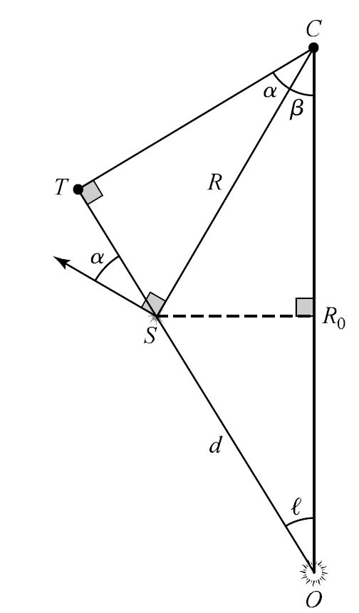
Fig. 5.17 The geometry of differential rotation in the Galactic plane, using relative locations for the Sun (point \(O\)), Galactic center (point \(C\)), and a star (point \(S\)) located a distance \(d\) from the Sun. Useful angles are the Galactic longitude \(\ell\) of the star, and \(\alpha\) and \(\beta\) as auxillary angles. The direction of motion reflect the clockwise rotation of the Galaxy as viewed from the NGP. Image Credit: Carroll & Ostlie (2007).#
Assume that the Sun is position at point \(O\) and a star is at point \(S\), where both are orbiting the Galactic center at point \(C\) in the Galactic midplane. The velocity vector between the Sun and the star is the relative velocity between the two objects. To compare the observed-velocity vector to the object’s true velocity with the Galactic center, it is necessary to consider the difference between the motions of the star and Sun. In practice, the radial and proper motion have to be measured so that the full space velocity can be determined. Note that the proper motion is converted into the transverse velocity only if the distance \(d\) to the star is known.
If the line of sight is in the direction of the Galactic longitude \(\ell\) and if \(\Theta(R)\) is the orbital velocity as a function of the distance from the Galactic center, then the relative and transverse velocities of the star are,
where \(\Theta_o\) is the orbital velocity of the Sun (or the LSR) in the idealized case of perfectly circular motion and $\alpha is an auxillary angle. Defining the angular-velocity curve to be
the relative radial and transverse velocities become
From Figure 5.17, consider the right triangle \(\Delta OTC\) and we find,
Substituting these relations into the velocity equations, we have
Although the Sun’s motion around the Galactic center is not perfectly circular, its peculiar velocity relative to the LSR is small compared to \(\Theta_o\). To a first approximation, the above equation provide a reasonable estimate of \(\Omega = \Omega(R)\) if the other parameters are known. However, the distance \(d\) can be hard to measure for many objects and will depend on which distance method (e.g., parallax, Cepheids, etc.) is the most reliable.
Another complication arises because of the effects of interstellar extinction. Our ability to observe Galactic structure to great distances is severely limited at visual wavelengths. Unless we have a special window of observations (e.g., Baade’s window), we are restricted to seeing stars out to a few \(1000\ \rm pc\) from the Sun. One important exception to this constraint is the 21-cm wavelength of H I. Virtually the entire Galaxy is optically thin to 21-cm radiation, which makes that wavelength band a valuable tool for studying Galactic structure.
Oort derived a set of approximate equations for \(v_r\) and \(v_t\) that are valid only in the region near the Sun. These alternative formulae are still able to provide a surprising amount of information about the large-scale structure of the Galaxy.
We make the assumption here that \(\Omega(R)\) is smoothly varying (i.e., differentiable) function of \(R\) so that the Taylor expansion of \(\Omega(R)\) about \(\Omega_o(R_o)\) is given by
To first order, the difference between \(\Omega\) and \(\Omega_o\) is
and the approximate value of \(\Omega \simeq \Omega_o\). If we use the identity \(\Omega = \Theta/R\), then the velocity equations become (with some rearrangement)
From Fig. 5.17, we see that
where the latter result is due to the small-angle approximation (i.e., \(\cos{\beta} \simeq 1\)), since \(d\ll R_o\) implies that \(\beta \ll 1\ \text{radian}\). Using the appropriate trigonometric identities and defining the Oort constants
Then, we have
For stars in the directions \(\ell = 0^\circ\) and \(\ell = 180^\circ\), the lines of sight are perpendicular to their motions relative to the LSR. AS a result, the radial velocity must be zero. For \(\ell = 90^\circ\) or \(270^\circ\), the stars begin observed are essentially the same circular orbit as the Sun and are moving with the same speed and \(v_r = 0\ \rm km/s\).
At intermediate angles, the situation is somewhat more complicated.
If we assume that in the solar neighborhood, \(\Omega(R)\) is monotonically decreasing outward, then at \(\ell = 45^\circ\), the observed star is closer to the Galactic center and is “outrunning” the Sun. Therefore, we measure a positive radial velocity as the star is moving away from the Sun (relatively speaking). The same is true at \(\ell = 225^\circ\) due to symmetry.
For \(\ell = 135^\circ\), The Sun is “overtaking” the star, which results in a negative radial velocity as the star appears to moving toward the Sun. The same is true at \(\ell = 315^\circ\) due to symmetry.
This results in a double sine curve, where a similar analysis of the transverse velocity also produces a double sine curve (with an additive constant). For a sample of stars (all with similar distances \(d\)), the amplitudes of the \(v_r\) and \(v_t\) give the Oort constants \(A\) and \(B\), respectively.
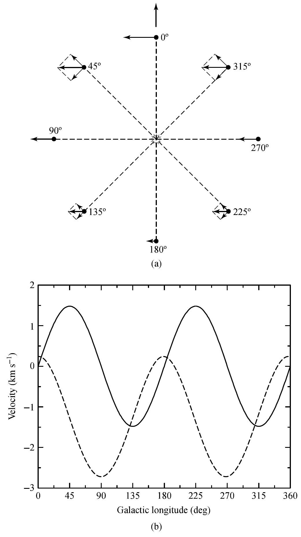
Fig. 5.18 (a) The differential rotation of stars near the Sun is revealed through the dependence of radial and transverse velocities on Galactic longitude. (b) Radial velocity is proportional to \(\sin{2\ell}\) (solid), and transverse velocity is a function of \(\cos{2\ell}\) (dashed). The curves depict stars located \(100\ \rm pc\) from the Sun with \(A = 14.8\ \rm km/s/kpc\) and \(B=-12.4\ \rm km/s/kpc\). Image Credit: Carroll & Ostlie (2007).#
It is now possible to derive several important relationships between the Oort constants \(A\) and \(B\), and the local parameters of Galactic rotation \((R_o,\ \Theta_o,\ \Omega_o,\ [d\Theta /dR]_{R_o})\). From the equations for the Oort constants, we immediately find that
Another useful relation can be found by considering the largest radial velocity seen along the line of sight at a constant Galactic longitude \(\ell\). Consider a star with the maximum observable radial velocity at point \(T\) (i.e. the position where \(\alpha = 0^\circ\)). It is at this tangent point that the distance to the Galactic center will be a minimum and \(\Theta(R)\) will be a maximum (under the assumption that \(\Theta(R)\) is monotonically decreasing from the center outward). The orbital velocity vector is directed along the line of sight at that position. This minimum distance from the Galactic center is given by
and the maximum radial velocity is
For Galactic longitudes near but less than \(90^\circ\) (or near but greater than \(270^\circ\); inside the solar circle), then \(d\ll R_o\) \(R\sim R_o\), and \(\Theta(R)\) can be expressed in terms of a Taylor expansion about \(\Theta_o\):
Substituting \(\Theta(R_{\rm min})\) into the expression for \(v_{\rm r,max}\), retaining the first-order terms, and making use of equation for the Oort constant \(A\), we find
One last relation associates \(A\) and \(B\) with the dispersions of peculiar velocities in the \(R\) and \(\theta\) directions:
Because \(A\) and \(B\) provide critical information about Galactic differential rotation in the solar neighborhood, considerable effort is spent into determining these constant. The Gaia spacecraft (launched in 2013) has allowed improved measurements of the Oort constants (Bovy 2017) as
5.4.5. Hydrogen 21-cm Line as a Probe of Galactic Structure#
To determine the large-scale velocity structure of the Galactic disk, we must find more general expression for \(v_r\) and \(v_t\) that do not rely on first-order Taylor series expansions. The 21-cm emission from H I is able to penetrate virtually the entire Galaxy, which makes it an indispensible tool in probing the structure of the Milky Way. By measuring \(v_r\) as a function of \(\ell\), the Galactic rotation curve can be determined provided that the distance (from the Sun) of the emitting region can be found.
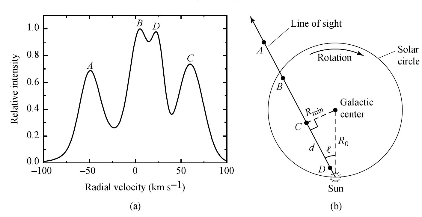
Fig. 5.19 (a) A typical 21-cm H I profile. (b) The line profile by observing several gas clouds along a particular line of sight. Because of differential Galactic rotation, each cloud has a different radial velocity (relative to the Sun). Image Credit: Carroll & Ostlie (2007).#
When a specific cloud is encountered along the line of sight, the wavelength of the radiation from that cloud is Doppler shifted because of the effects of differential Galactic rotation. The intensity of the radiation at a given wavelength (or velocity) is proportional to the number of hydrogen atoms along the line of sight in the cloud. The peaks in a typical 21-cm H I line profile correspond to the H I clouds along the line of sight (but at different distances) in the Galaxy.
The principle difficulty in using 21-cm radiation to determine \(\Omega(R)\) \((\text{and } \Theta(R))\) lies in measuring \(d\). This problem can be overcome by selecting the largest radial velocity measured along each line of sight, which must originate in the region \(R_{\rm min}\) from the Galactic center (i.e., \(d = R_o \cos{\ell}\)). By measuring \(v_{\rm r,max}\) for \(0^\circ < \ell < 90^\circ\) and \(270^\circ < \ell < 360^\circ\), we can determine the rotation curve within the solar Galactocentric radius.
The above technique does not work for the intermediate longitudes \(90^\circ < \ell < 270^\circ\) because there is no unique orbit for which a maximum radial velocity can be observed. The method also tends to break down near \(\ell =90^\circ\) and \(\ell = 270^\circ\) because v_r becomes rather insensitive to changes in distance from the Sun. For longitudes within approximately \(20^\circ\) from the Galactic center, the clouds that have markedly non-circular motions exist in that region, where this creates problems so that the assumptions underlying the preceding analysis are not valid.
5.4.6. The Flat Rotation Curve and Evidence of Dark Matter#
To measure \(\Theta(R)\) for \(R> R_o\), we must rely on objects available in the Galactic plane (e.g., Cepheids) for which we can directly obtain distances. These data suggests that the rotation curve of the Galaxy dose not decrease significantly with distance beyond \(R_o\) and may actually increase somewhat. This means that near \(R_o\) the Oort constants are related by \(A<-B\). Combining all the available data in 1985, a possible form for the rotation curve of the Galaxy is shown in Figure 5.20.
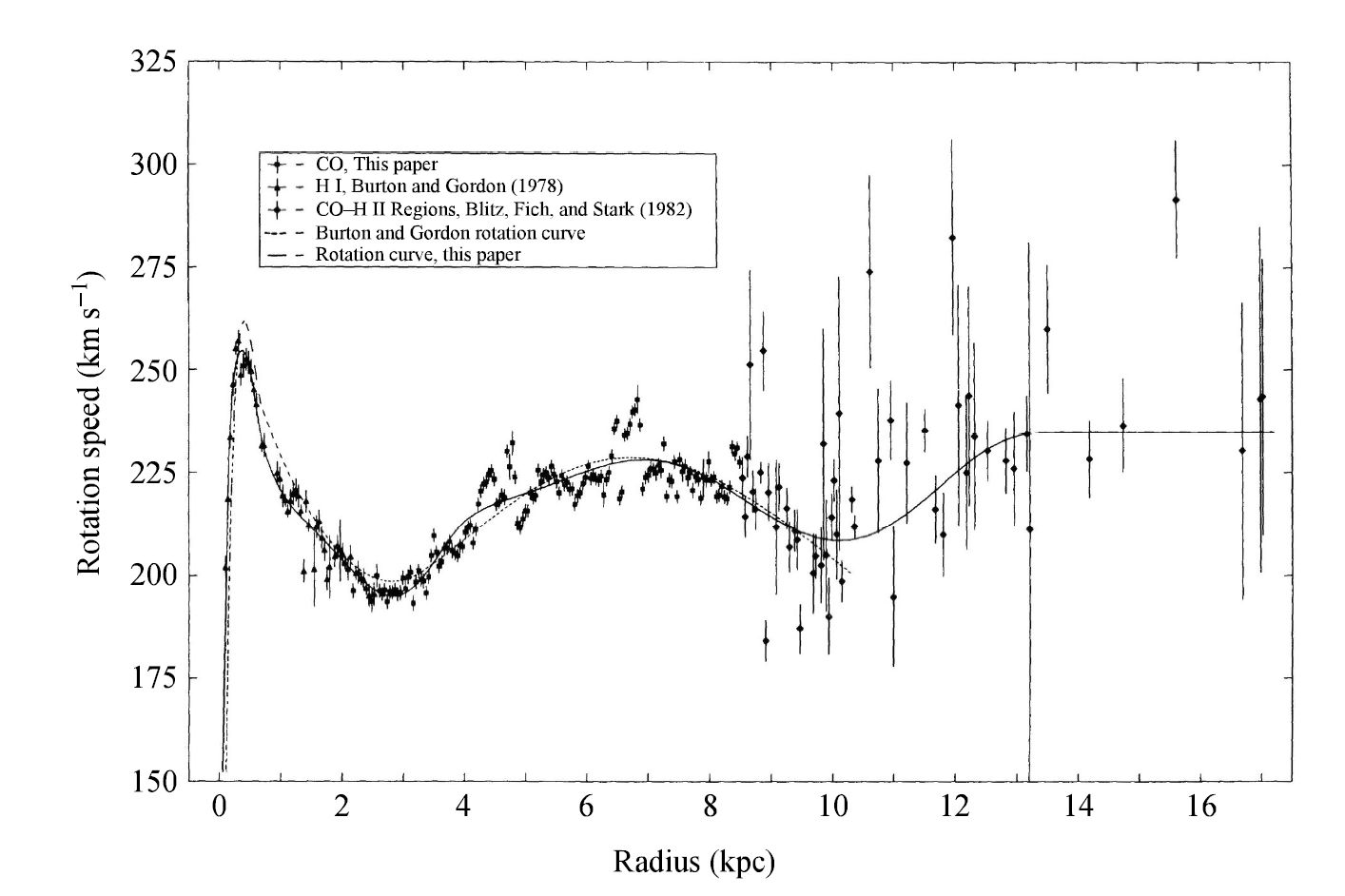
Fig. 5.20 The rotation curve of the Milky Way, where the 1985 IAU standard values of \(R_o = 8.5\ \rm kpc\) and \(\Theta_o = 220 \rm km/s\) were assumed. Image Credit: Carroll & Ostlie (2007). The figure was adapted from Clemens (1985).#
It came as a great surprise to astronomers to discover that the Galactic rotation curve is essentially constant beyond \(R_o\). According to Newtonian mechanics, if most of the mass where interior to the solar circle, the rotation curve should drop off as \(\Theta \propto 1/\sqrt{R}\) (i.e., Keplerian motion). The fact that it does not implies that as significant amount of mass exists beyond \(R_o\). This result was particularly unexpected since most of the luminosity of the Galaxy is produced by matter residing inside \(R_o\).
The data for the Milky way are supported by observations of other spiral galaxies (e.g., those obtained by Rubin et al. in the late 1970s). Figure 5.21 shows a spectrograph slit superimposed on NGC 2998 and a portion of the spectrum in the wavelength region near \(\rm H\alpha\). The left side of the slit recorded blueshifted light, while the light on the right side was redshifted. The Doppler shifts were translated in to radial velocities, and a corresponding rotation curve was determined.
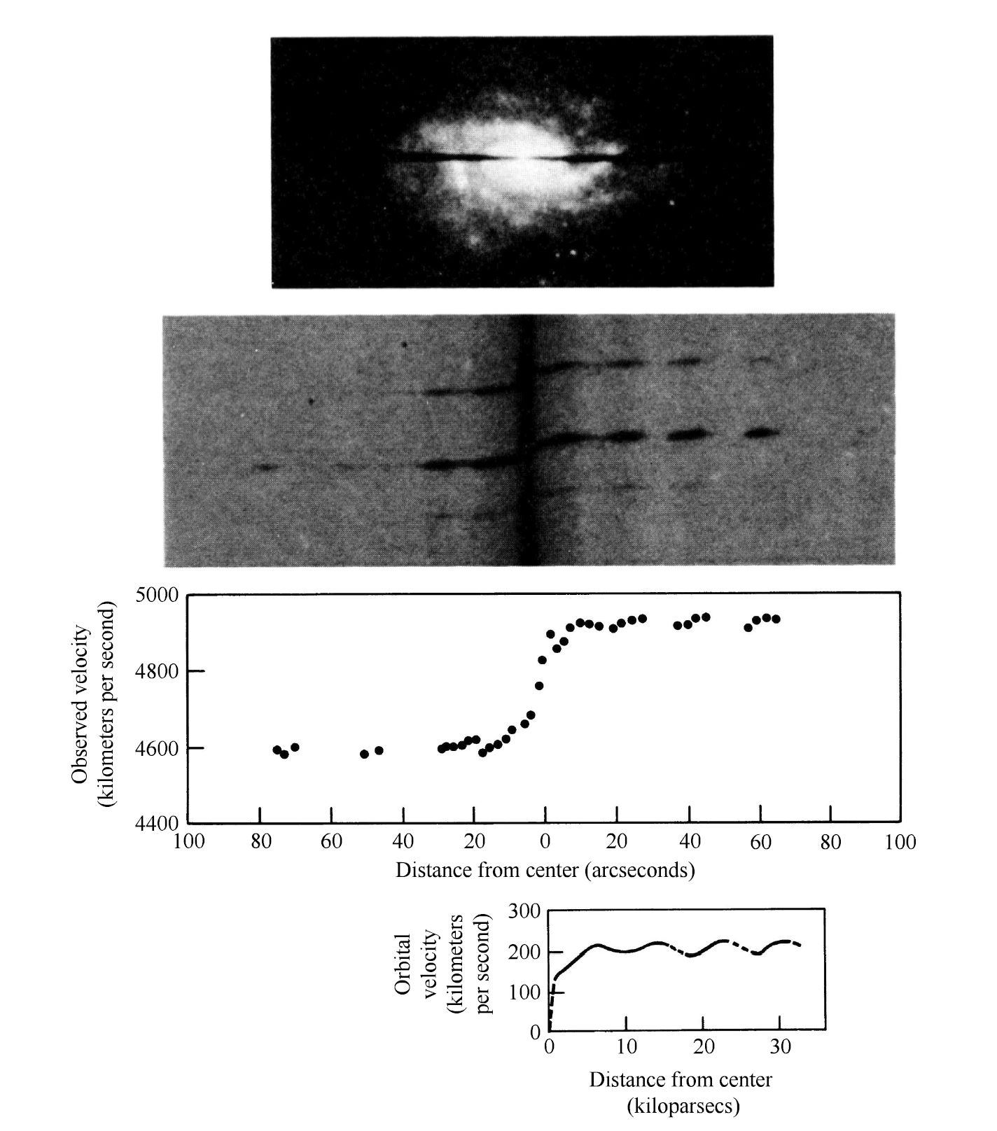
Fig. 5.21 The rotation curve of NGC 2998 measured using a slit spectrograph with the \(\rm H\alpha\) wavelength region. The entire galaxy is receding from us at a speed of \(4800\ \rm km/s\). Image Credit: Carroll & Ostlie (2007). The figure was adapted from Rubin (1983).#
Similar rotation curves have also been measured for a number of other spiral galaxies. With the exception of the innermost regions, there is a rapid rise in rotation speed with distance out to a few \(\rm kpc\) from the center. When \(\Theta \propto R\), the angular speed \(\Omega\ (= \Theta/R)\) is a constant and all stars have the same orbital period, which is referred to as rigid-body rotation, about the Galactic center. Beyond a few \(\rm kpc\), nearly flat rotation curves continue out the edge of the measurements.
The Galactic rotation depends on the mass distribution and thus, a great deal can be learned about the matter in galaxies by studying these curves. For example, rigid-body rotation near the Galactic center implies that the mass must be roughly spherically distributed and the density nearly constant. On the other hand, flat rotation curves suggest that the bulk of the mass in the outer portions of the Galaxy are spherically distributed with a density law that is proportional to \(1/r^2\).
If we assume that \(\Theta(r) = V = \text{const.}\), then we can use the equations for the centripetal force and Newton’s law of gravity to identify the mass as a function of radius \(M_r\). The force acting on a star of mass \(m\) due to the mass \(M_r\) of the Galaxy interior to the star’s position at \(r\) is
assuming spherical symmetry. Solving for \(M_r\), we find
and differentiating with respect to radius \(r\),
The equation for mass conservation in a spherically symmetric system is given as
where we see that the mass density in the outer regions of the Galaxy can be determined by
The \(1/r^2\) density dependence is very different from the form determined by star counts in the portion of the Galaxy beyond \(R_o\). The number density of stars in the luminous stellar halo is believed to vary as \(1/r^{3.5}\), which is a much more rapid drop-off than is evident from the flat rotation curve.
It was this discrepancy that surprised astronomers. It appears that the majority of the mass in the Galaxy is in the form of nonluminous (dark) matter. Only through its gravitational influence on the luminous component of our Galaxy, satellite galaxies (e.g., the LMC and SMC), and through gravitational lensing from background sources does the dark matter become apparent.
The mass density is modified by many astronomers to prevent it from diverging near the center and to instead approach a constant value. This model is consistent with the observational evidence of rigid-body rotation. As a result, one commonly used density profile for the Milky Way’s dark matter halos is of the form,
where \(\rho_o\) and \(a\) are fitted parameters to the overall rotation curve.
Note
For \(r \gg a\), the \(1/r^2\) dependence is obtained, while \(\rho \sim \text{constant}\) when \(r \ll a\). A similar profile is often used for modeling other galaxies as well, with different choices for \(\rho_o\) and \(a\).
This mass density profile cannot be correct to arbitrarily large values of \(r\) because the total amount of mass in the Galaxy would increase without bound since \(M_r \propto r\). As a result, the density function for the dark matter halo must eventually terminate, or at least decrease sufficiently rapidly that the mass integral \(\int_0^\infty \rho(r)\ 4\pi r^2\ dr\) remains finite.
An alternative form of the dark matter halo density distribution was proposed by Navarro et al. (1996). Using a commonly assumed form of dark matter dynamics known as cold dark matter (CDM), Navarro et al. ran numerical simulations of the formation of dark matter halos over a wide rang eof size and mass scales (ranging from dwarf galaxies to rich clusters of galaxies). Their simulations revealed a “universal” profile of the form,
which was applicable over an enormous range with appropriate choices of \(\rho_o\) and \(a\). The NFW density profile behaves approximately like a \(1/r^2\) profile over much of the halo, but is shallower \((\sim 1/r)\) near the center and steeper \((\sim 1/r^3)\) near the edge of the halo. Even though the NFW profile decreases more rapidly with increasing \(r\) (compared to the previous profile), it can be shown that the total mass contained within the profile is still not bound.
In reality, other galaxies exist in our universe besides the Milky Way, and their mass density functions may overlap our own. As a result, their dark matter halos may actually merge into intergalactic space.
5.4.7. Some Methods for Determining Distances#
There are motion-based methods of determining distances within the Milky Way, where the most important of which is the moving cluster method. Since the stars are gravitationally bound to one another in a stellar cluster, they move through space collectively. By recording the changing positions of the group members over time (due to the cluster’s bulk motion), it is possible to determine their direction of motion.
After removing the effects of the Sun’s peculiar motion, we can trace the directional vectors through space, which gives the appearance that each star is moving toward (or coming from) a convergent point. This is simply the illusion that parallel lines appear to converge at infinity, a phenomenon used to give the illusion of three dimensions in a drawing or painting (e.g., railroad tracks or a river emanating from a page).
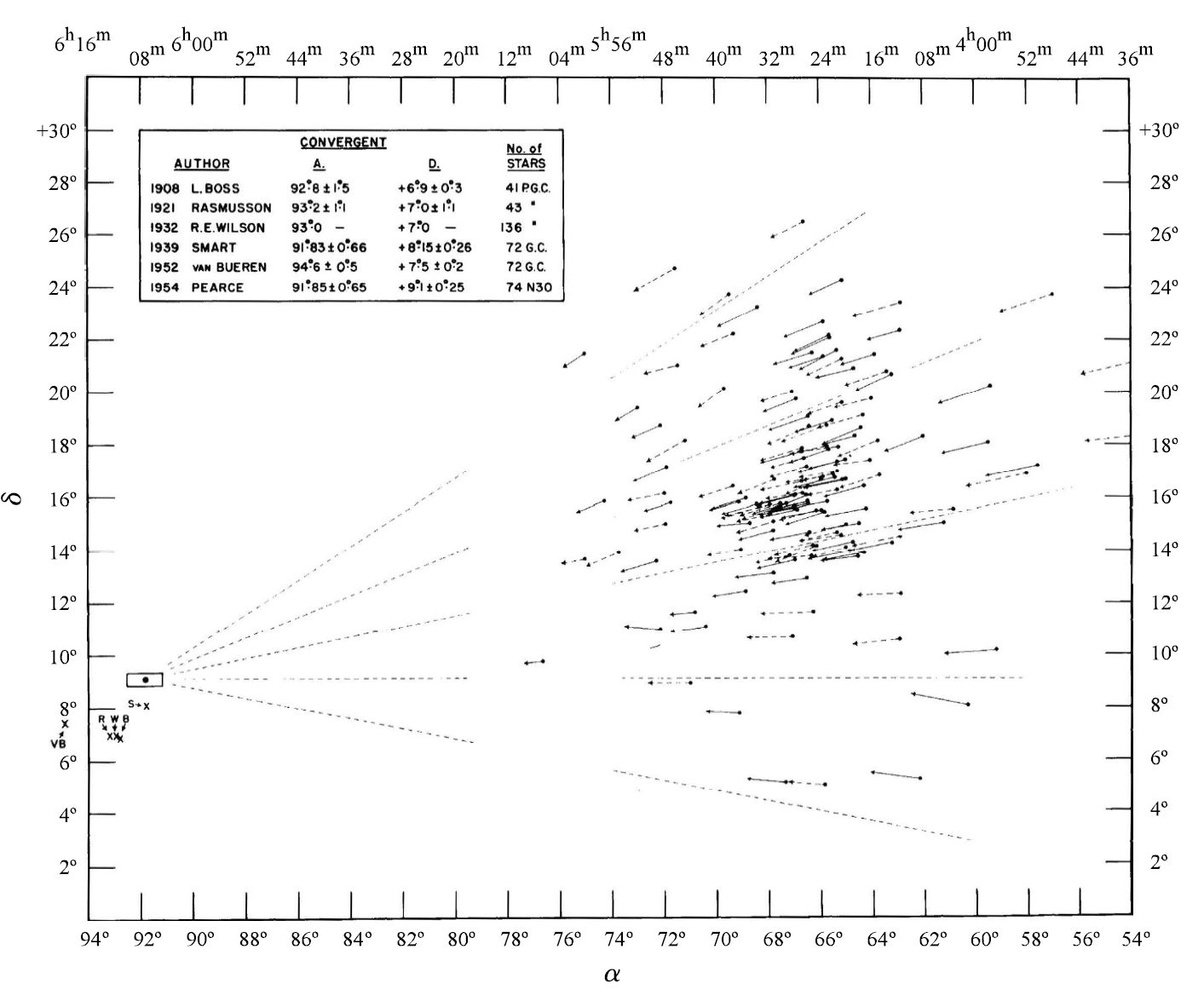
Fig. 5.22 The apparent motion of the Hyades cluster across the celestial sphere. Image Credit: Carroll & Ostlie (2007). The figure was adapted from Elementary Astronomy by Struve, Lynds, & Pillans (1959).#
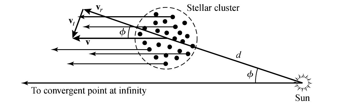
Fig. 5.23 The space motion of the cluster is directed toward the convergent point, where the velocity vector may be decoupled from its radial and tranverse components. Image Credit: Carroll & Ostlie (2007).#
Consider the cartoon in Figure 5.23, the angle between the cluster and the convergent point (as seen from the Sun) must be the same as the angle between the line-of-sight to the cluster and its space velocity vector \(\mathbf{v}\); this statement is valid only because the convergent point is taken to be at infinity. Decomposing the space velocity into its perpendicular components, the radial velocity is given by \(v_r = v\cos{\phi}\), and the transverse velocity is \(v_t = v\sin{\phi}\). Dividing these components yields the relation,
The transverse velocity is observed as the proper motion \(\mu\ (=v_t/d)\), and the distance to the cluster can be determined from using the direction to the convergent point \(\phi\), the average radial velocity \(\langle v_r \rangle\) of the cluster members, and the average of their proper motions \(\langle \mu \rangle\). Combining these elements gives,
Expressing \(d,\ v_r,\ \text{and } \mu\) in units of \(\rm pc,\ km/s,\ \text{and } \text{arcsec/yr}\), we get
The above technique has been used to determine the distances to several clusters, including the Hyades with its \({\sim}200\) members, the Ursa Major group (60 stars), and the Scorpio-Centaurus group (100 stars). The distance to the Hyades is found to be \(46\pm 2\ \rm pc\) using the above method, which is in excellent agreement with other distance determinations (e.g., trigonometric parallax). The Gaia space astrometry mission data yielded a value of \(47.50 \pm 0.15\ \rm pc\) (Röser, Schilibach, & Goldman (2018)).
Once the distance to the Hyades was determined, the absolute magnitudes of its members could be found and a calibration of its main sequence could be performed. By comparing the apparent magnitudes of other cluster H-R diagram main-sequences to the Hyades, it is then possible to find the distance moduli of the other clusters (see slideshow by Ellie Lincoln @ GSU for limitations).
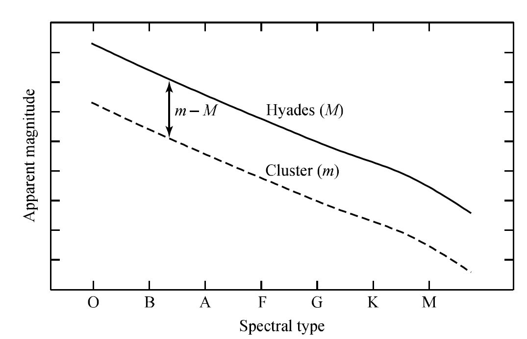
Fig. 5.24 The distance modulus of a cluster can be determined by shifting the cluster’s main sequence vertically in the H-R diagram until it conicides with the known absolute magnitude of the Hyades’ main sequence. This method is known as main sequence fitting. Image Credit: Carroll & Ostlie (2007).#
Assuming that the amount of interstellar extinction is known (e.g., from reddening data), the distances to other clusters can be measured, especially if the radial velocities of cluster members are hard to measure (i.e., due to crowding or faintness). This distance technique is known as main sequence fitting and is similar to spectroscopic parallax. However, main sequence fitting is a more precise procedure because it relies on a large number of stars along the main sequence rather than a single object.
Identifying variable stars (e.g., RR Lyraes or Cepheids) in clusters of known distances provides a means of determining the intrinsic luminosities of these stars more accurately. Once the luminosities of the variable stars have been calibrated, they can be used to determine other distances (e.g., distance to globular clusters). Historically, the Hyades provided the foundation for virtually all distance estimates (both Galactic and extragalactic) beyond about \(100\ \rm pc\) from Earth.
The ability to measure distances directly (via trigonometric parallax) relies on the diameter of Earth’s orbit. If the length of the baseline could be increased, it would be possible to extend the method to objects farther away. This is accomplished by using the peculiar motion of the Sun (or secular parallax) with respect to a stellar cluster, whose members have similar properties (e.g., similar spectral types, distances, and space motions). The overall solar motion of \(13.4\ \rm km/s\) is equivalent to \(2.8\ \rm AU/yr\), where the Sun’s motion over several years provides a significantly larger baseline compared to Earth’s orbit. This larger baseline can then be used to determine the average distance to the cluster.
5.5. The Galactic Center#
Observations of the Galactic center pose a challenge due to the abundance of gas and dust in the Galactic plane, which results in \(>30\) magnitudes of extinction at visible wavelengths. The line of sight from the Sun to the center (located only \(30\ \rm pc\) above the midplane and \(8\ \rm kpc\) from the center) traverses nearly the maximum possible amount of interstellar material.
Interestingly, the solar peculiar velocity has an appreciable component perpendicular to the Galactic plane \((w_\odot = 7.2\ \rm km/s)\), which means that the Sun will reach \({\sim}85\ \rm pc\) above the plane in \(15\ \rm My\). This will place it above most of the obscuring material. If humanity is still inhabiting the Earth at that time, our descendants will enjoy a spectacular view of a dense stellar cluster near the Galactic center.
5.5.1. The Mass Distribution Near the Galactic Center#
To view the Galactic center today, we are forced to make (most of) our observations in the infrared, microwave, and radio (i.e., \(\lambda > 1\ \mu \rm m\)). Despite our difficulty in seeing the Galactic center in visible wavelengths, we have been able to construct an image of the Galactic nucleus that depicts a history of violent events and exotic phenomena.
For investigations of the Galactic core, IR observations use wavelengths centered at \(2.2\ \rm \mu m\) (i.e., the \(K\) band). This wavelength band is used due to the large number of old (Pop. I) K and M giant stars \((T_e \sim 4000\ \rm K)\) that exist near the Galactic central region and are readily observable at \(2.2\ \rm \mu m\). Using the \(K\) band to study the brightness of the central cluster (and an appropriate mass-to-light ratio, \({\sim}1\ M_\odot/L_\odot\)), it appears that the mass density of stars rises toward the center as \(r^{-1.8}\) down to a radius of \(0.1-1\ \rm pc\). This is roughly the type of distribution that would be expected on dynamical grounds (i.e., a region of rigid-body rotation).
The stars in the central region are very close together, particularly when compared with the distance between stars in the solar neighborhood. As a result, close encounters are fairly frequent and occur on average once every \({\sim}10^6\) years. From these close encounters, the constant exchange of mechanical energy between stars has generated a nearly isothermal velocity distribution (i.e., the stars in the sample have a velocity distribution that is approximately Maxwellian). In a truly isothermal stellar gas, the mass density distribution is \(r^{-2},\) which is close to the \(r^{-1.8}\) variation that is observed.
The observed density distribution of an isothermal stellar gas is inconsistent with measurements of stellar velocity within \(2\ \rm pc\) from the center. Sellgren et al. (1990) observed using the \(2.3\ \rm \mu m\) molecular absorption band of \(\rm CO\) found in the spectra of cool K and M giants. They found that although the velocity distribution is fairly isothermal from several \(100\ \rm pc\) down to a couple of parsecs from the center, velocities begin to increase significantly as the distance to the center continues to decrease. This suggests that either
the stellar density must rise substantially faster than \(r^{-2}\) toward the center (at least as steeply as \(r^{-2.7}\)), or
there must be a great deal of mass occupying a very small volume near the middle of the cluster.
Schödel et al. (2002) followed the orbits of stars very close to the Galactic center. In particular, the star known as S2 has an orbital period of \(16.0518\ \rm yr\), an orbital eccentricity \(e=0.88466\), and a perigalacticon distance of \({\sim}120\ \rm AU\), or 17 light-hours, after including the effects of Schwarzschild precession (GRAVITY Collaboration (2018)). This size is only a few times the semimajor axis of Pluto’s orbit!
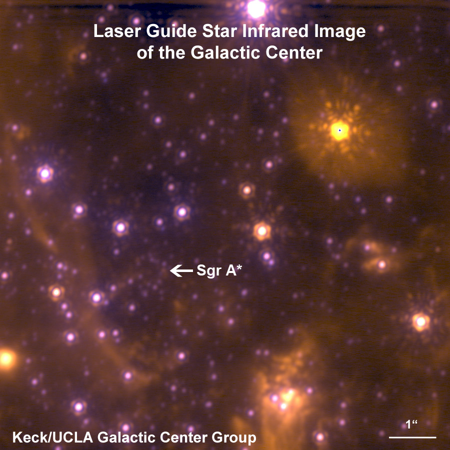
Fig. 5.25 Image of the Galactic center showing the position of Sgr \(A^\star\). Image Credit: UCLA Galactic Center Group.#
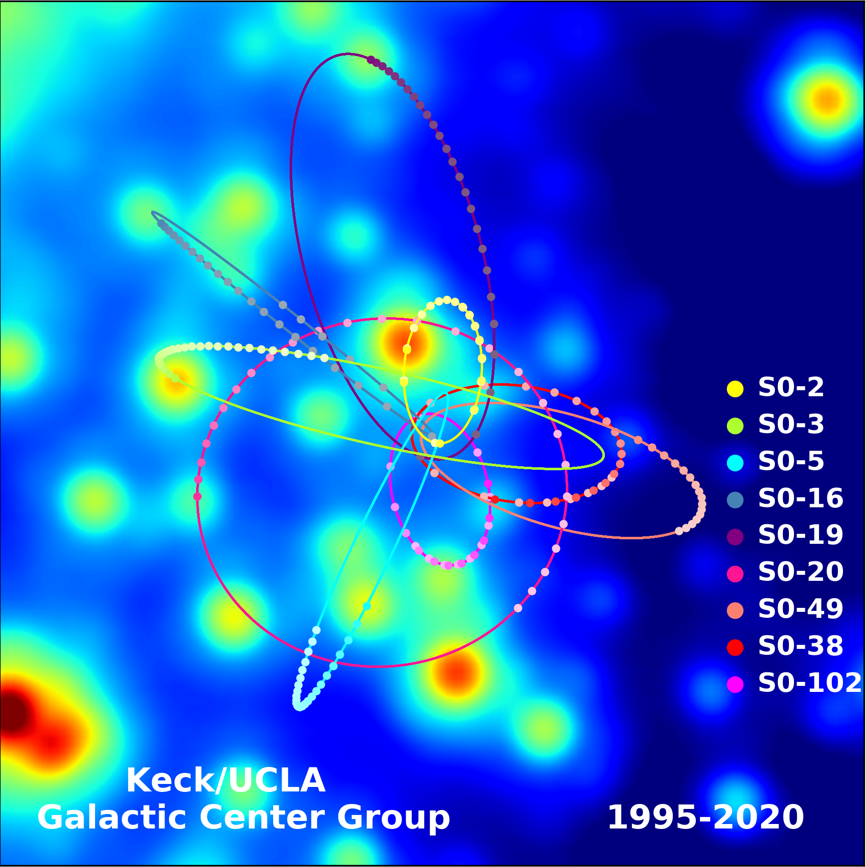
Fig. 5.26 Observations of the Galactic center showing the orbits of stars (including S2) around Sgr \(A^\star\). Image Credit: UCLA Galactic Center Group.#
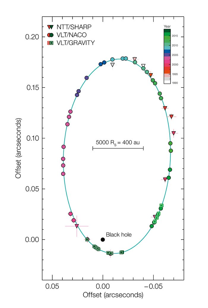
Fig. 5.27 Orbit of S2 around the Galactic center. Image Credit: ESO/MPE/GRAVITY Collaboration.#
Exercise 5.3
The mass interior to the orbit of S2 can be estimated using Newton’s version of Kepler’s 3rd law.
What is the approximate mass at the Galactic center?
From the known orbital parameters for S2, we can estimate its semimajor axis using its perigalacticon distance of \(120\ \rm AU\) and the measured eccentricity. As a result, we find
for the semimajor axis \(a_{\rm S2}\). The orbital period of S2 is \(16.0518\ \rm yr\), where we can determine the interior mass in solar units if we use a semimajor axis in AU, orbital period in \(\rm yr\), and let \(G=4\pi^2\). Then, we can find the interior mass by
A more precise calculation gives \(M = 4.1 \times 10^6\ M_\odot\) by GRAVITY Collaboration (2018). Note that this is consistent (within \(2\sigma\)) with other prior measurements made by Ghez et al. (2008), which found \(M = 4.5\ (\pm 0.4) \times 10^6\ M_\odot\).
The luminosity distribution of the stars near the Galactic center peaks within a few arcseconds \(({\sim}0.1\ \rm pc)\) of a infrared object known as IRS 16 (for infrared source). It was during a lunar occultation that IRS16 was resolved into at least 15 very luminous point-like sources that are most likely individual stars.
These sources appear to be hot stars with brightnesses in excess of \(10^6\ L_\odot\). They may be O and B stars, but with luminosities that are much greater than expected for normal stars. The UV fluxes of these stars are absorbed by the surrounding gas and dust, then reradiated in the IR. These stars might be Wolf-Rayet, which are extremely rare in other parts of the Galaxy. Wolf-Rayets are massive stars, where they must have evolved to their present states very rapidly in which a burst of star formation must have occurred within the past \(10\ \rm Myr\).
However, a burst of star formation seems to contradict observations that the gas and dust density is very low and there is no observed on-going star formation in that region today. On the other hand, the presence of high-velocity gas \(({\sim}700\ \rm km/s)\) near IRS 16 supports the Wolf-Rayet idea in which some researchers suggest that the gas may have been ejected as a stellar wind by one of the stars. As an alternative explanation, others point out that it is possible that the high-velocity gas could simply be falling in toward the Galactic center rather than being ejected from it. The velocity structure of the gas does not appear to be consistent with the acceleration expected of Wolf-Rayet winds with increasing distance from the star, where the gas velocity appears to decrease with distance.
Note
Determining whether the gas is falling in toward the Galactic center or being ejected from it requires information about the orientation of the gas trajectories relative to the line-of-sight. This is something that is often difficult to determine in practice.
IRS 16 does not appear to have sufficient mass to account for the rise in orbital velocities near the center. It seems that whatever the origin of this extremely localized mass distribution, it must have an overall luminosity that remains below our threshold of detectability. One possibility is that the mass is composed of a very dense cluster of brown dwarfs and/or more massive neutron stars. Even in the case of neutron stars, interactions with high-mass stars would eject the lower-mass neutron stars from the center in \(< 10^8\ \rm yr\). This would have the additional effect that the most massive members of the cluster would “sink” to the center of the Galaxy’s gravitational well, which is not observed.
5.5.2. Radio Sources in Sagittarius#
Karl Jansky (in the 1930s) first discovered that a radio source was located in the direction of Sagittarius, but extensive observations of the Galaxy in the radio were delayed until after World War II, where major advances in radio technology were also made over the course of WWII. Since that time, the Galactic center has been the site of numerous studies at radio wavelengths.
Radio observations of H I clouds reveal a nuclear disk of neutral gas occupying a region between a few hundred parsecs and about \(1\ \rm kpc\) from the center. The disk appears to be tilted slightly with respect to the Galactic plane and contains clouds with significant non-circular motions.
Galactic lobes of ionized gas have also been observed within the central few hundred parsecs. The lobes (dimensions of \(10\ \rm pc\) by \(200\ \rm pc\)) are elongated and oriented nearly perpendicular to the Galactic plane and may represent material begin ejected from the center. However, the data may also be consistent with infalling material.
One of the more unusual feature of the radio emission originating in the central region of the Galaxy is the set of filaments that stretch for \(20\ \rm pc\) in a direction perpendicular to the Galactic plane and then make an almost right-angle turn. An inspection of this 20-cm radio structure (located near \(\ell \sim 0.18^\circ\)) suggests that magnetic fields may be responsible for the unusual pattern. The radiation is linearly polarized and appears to be synchrotron emission. From the intensity of the radiation and the amount of polarization, the strength of the Galactic magnetic field in that region is probably between \(10^{-8}-10^{-6}\ \rm T\), which is \({\sim}2-4\) orders of magnitude weaker than Earth’s magnetic field. A similar feature has been discovered south of the Galactic plane, where these structures seem to be part of a “halo” of streamers and filaments that may correspond to mass outflow from the Galactic center.
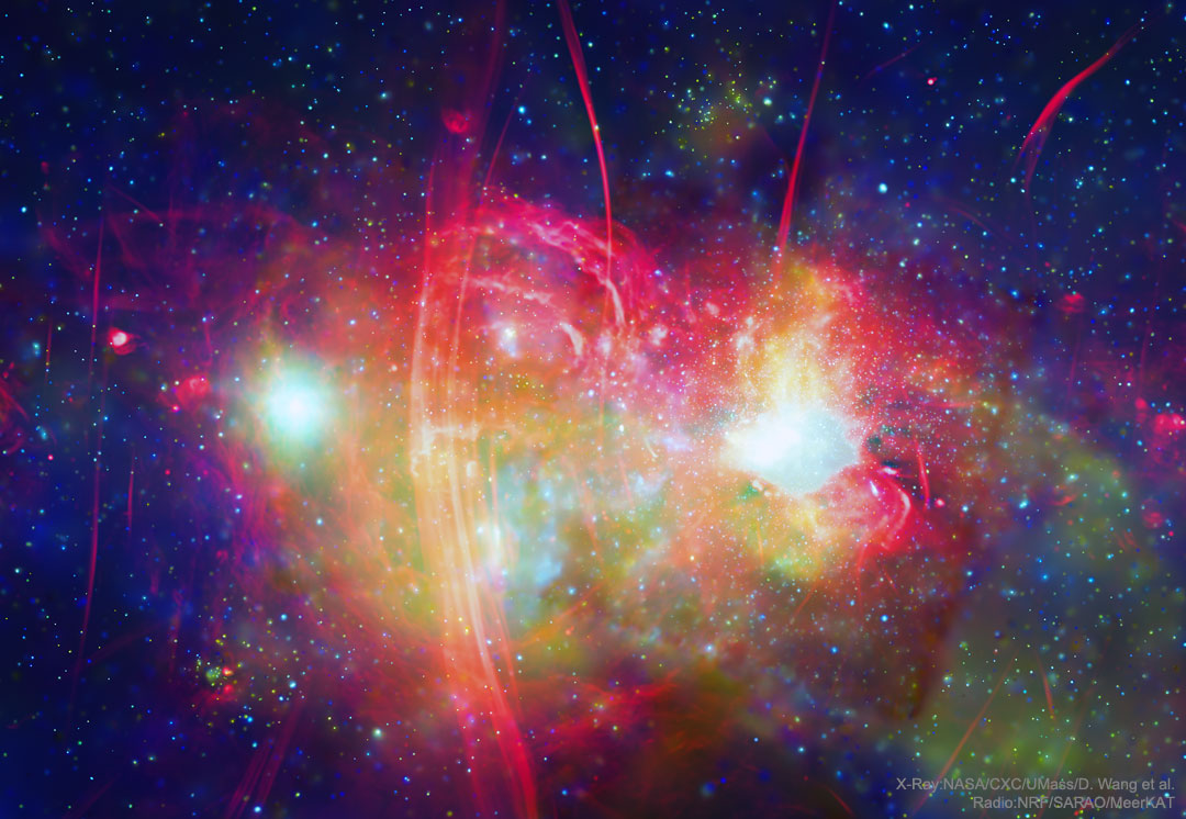
Fig. 5.28 Multi-wavelength image of the Galactic center. Parallel radio filaments known as the Arc mark the unusual pattern in radio emission. Image Credit: X-Ray: NASA, CXC, UMass, D. Wang et al.; Radio: NRF, SARAO, MeerKAT.#
The inner \(8\ \rm pc\) of the Galaxy contains the radio source designated as Sagittarius A (Sgr A). With the increase in resolving power provided by interferometry and radio arrays (e.g., VLA), it has become possible to study the structure of the Sgr A complex down to an angular resolution of \({\sim}0.2\ \rm mas\), corresponding to linear dimensions of \(<2\ \rm AU\).
The largest feature of the complex is the molecular circumnuclear ring, which is a toroidal structure with an inner radius of \(2\ \rm pc\) and an outer radius of \(8\ \rm pc\) that is inclines some \(20^\circ\) with respect ot the Galactic plane. The inner edge of the ring exhibits some warping and the ring thickness increases from \(0.5\ \rm pc\) at its inner edge to \(2\ \rm pc\) at a Galactocentric distance of \(7\ \rm pc\).
This molecular ring has been observed at various wavelengths associated with several atoms and molecules (e.g., \(\rm H\ I\), \(\rm H_2\), \(\rm C\ II\), \(\rm O\ I\), \(\rm OH\), \(\rm CO\), \(\rm HCN\), and \(\rm CS\)). The ring is rotating about the Galactic center at a speed of \({\sim}110\ \rm km/s\), which is a value that is nearly independent of radius. From the collisional excitation of molecules and the intensity of emission, the estimated mass of the ring portion located between \(2-5\ \rm pc\) is \(1-3 \times 10^4\ M_\odot\).
The circumnuclear ring also shows evidence that some violent event occurred near the Galactic center in the relatively recent past. The inner edge of the ring is very sharp, where the number density of particles inside the central cavity is \(10-100\) times less than in the ring itself. Such a strong density discontinuity cannot be an equilibrium feature of the ring because the ring’s internal turbulence would destroy the discontinuity in less than \(10^5\ \rm yr\). Furthermore, the gas withing the cavity is largely ionized while the gas in the ring is in the form of neutral atoms and molecules. The amount of energy required to clear out the ring is on the order of \(10^{44}\ \rm J\), which is characteristic of a supernova explosion.
The ring shows other evidence of some past violent episode. For instance, material in the ring is very clumpy, which is a situation that cannot be maintained indefinitely because of the relatively rapid smoothing effects of cloud-cloud collisions. A study of the hydroxyl molecule \(\rm OH\) in portions of the ring indicates that the temperature of nearly \(2000\ \rm K\) is consistent with strong shocks that rapidly heated the molecules to temperature well above the values elsewhere in the ring.
Besides the circumnuclear ring, several other components have also been discovered within the Sgr A complex. Sgr A East is a nonthermal source with a shell-like appearance. It is generally accepted that Sgr A East is a young supernova remnant (SNR) that may be between \(100-5000\ \rm yr\) old. Sgr A West is located \(1.5^\prime\) from the center of Sgr A East and is an unusual \(\rm H\ II\) region (i.e., a thermal source) that looks very much like a “mini-spiral.” Finally, Sgr \(A^\star\) is a strong, unresolved radio point source that is located near the center of Sgr A West.
Note
A “nonthermal” source is one that does not emit its EM radiation in the form of a blackbody spectrum. On type of nonthermal emission is synchrotron radiation.
The location the Sgr A complex corresponds very closely with the brightness peak of the central stellar cluster. One component of IRS 16 is only \({\sim}1^{\prime\prime}\) west of Sgr \(A^\star\). If the two objects are the same distance from Earth and not simply aligned along the line-of-sight, then their angular separation translates into a linear separation of only \(0.04\ \rm pc\).
Although Sgr A West appears superficially much like the large-scale spiral pattern seen in the Milky Way’s disk, it is fundamentally very different. The western arc is just the ionized inner edge of the circumnebular ring, which is rotating about the center at \(110\ \rm km/s\). The other components of Sgr A West appear to be ionized filaments of matter that may be both rotating and falling in toward the central “bar” and the vicinity near Sgr \(A^\star\). These features may also be associated with a central magnetic field.
Exercise 5.4
The motion of gas in the central regions of the Galaxy can be used to estimate the amount of mass interior to the location of the gas. Note that this can be another check on our estimate of mass using stellar motions.
What is the total mass interior to a gas cloud that is \(0.3\ \rm pc\) from the Galactic center and has a measured velocity of \(260\ \rm km/s\)?
Assuming that the cloud’s motion is approximately circular, we can use the following expression for the interior mass,
This estimate is consistent with the mass estimate of the Galactic center using S2.
from scipy.constants import G, parsec

v = 260*1e3 #velocity of gas cloud in m/s
r = 0.3*parsec #radius of gas cloud from center in m
M_sun = 1.989e30 #Mass of the Sun in kg

M_r = v**2*r/G
print("The mass interior to the gas cloud is %1.2e M_sun." % (M_r/M_sun))
The mass interior to the gas cloud is 4.71e+06 M_sun.
5.5.3. An X-Ray Source in Sgr A#
Within the positional error bars, the radio Sgr A West region also coincides with a small continuous X-ray source. Although the estimates are uncertain due to extensive absorption along the line-of-sight, the X-ray source appears to have a characteristic temperature of \(T \sim 10^8\ \rm K\) and luminosities of \(10^{28}\ \rm W\) in the \(2-6\ \rm keV\) energy band (i.e., soft X-rays) and \(2\times 10^{31}\ \rm W\) between \(10\ {\rm keV}\) and \(10\ \rm MeV\). (i.e., hard X-rays).
Because the X-ray source is highly variable, it must be composed of one or a few objects whose diameters are \(\lesssim 0.1\ \rm pc\). The upper limit on the linear size is derived from the minimum amount of time required for information to travel across the object, assuming that the information travels at the speed of light. If one side of the source begins changing brightness, the opposite side can learn about the change and begin contributing to it oly after a time \(\Delta t \geq d/c\), where \(d\) is the diameter. Measuring \(\Delta t\) places the upper limit of \(0.1\ \rm pc\) on \(d\).
5.5.4. The Supermassive Black Hole in Sgr A*#
Two groups (GRAVITY collaboration and UCLA) have followed the orbits of individual stars to within \({\sim}120\ \rm AU\) of Sgr \(A^\star\). These observations have provided us with the critical data for accurately calculating the mass in the innermost region of the Galactic Center and perform critical tests of General Relativity (Hees et al. (2017); Witze (2018)). It now appears that Sgr \(A^\star\) can only be a supermassive black hole with a mass of \({\sim}4.1 \times 10^6\ M_\odot\). This implies that the Schwarzschild radius of the black hole is
from scipy.constants import G, c, astronomical_unit

AU = astronomical_unit
M_sun = 1.989e30 #Mass of Sun in kg
R_sun = 0.00465047*AU # radius of the Sun in m


R_SgrA_star = 2*G*(4.1e6 * M_sun)/c**2
print("The Schwarzschild radius of Sgr A* is %1.3f AU or %1.1f R_sun." % (R_SgrA_star/AU,R_SgrA_star/R_sun))
The Schwarzschild radius of Sgr A* is 0.081 AU or 17.4 R_sun.
Despite this small size, a collaboration of astronomers combined observations to form the Event Horizon Telescope (EHT) that uses interferometry to increase the diffraction-limited resolution to \(25\ {\mu as}\) (microarcseconds). On May 12, 2022, the EHT team announce the successful imaging of the accretion disk surrounding Sgr \(A^\star\). EHT announced a similar detection for the center of M87 only a few years prior.

Fig. 5.29 This is the first image of Sgr A*, the supermassive black hole at the centre of our galaxy. It’s the first direct visual evidence of the presence of this black hole. It was captured by the Event Horizon Telescope (EHT), an array which linked together eight existing radio observatories across the planet to form a single “Earth-sized” virtual telescope. Image Credit: Wikipedia:Event_Horizon_Telescope.#

Fig. 5.30 In this image of M87* taken on 11 April 2017 (a representative example of the images collected in a global 2017 EHT campaign), the shadow of a black hole is the closest we can come to an image of the black hole itself, a completely dark object from which light cannot escape. Image Credit: Wikipedia:Event_Horizon_Telescope.#
Producing the IR radiation detected from the ring and maintaining the degree of ionization seen inside the cavity require a UV luminosity of \(10^7\ L_\odot\) with an effective blackbody temperature of \(35,000\ \rm K\). The temperature is deduced from the strengths of IR emission lines of \(\rm S\ IV\), \(\rm O\ III\), and \(\rm Ar\ III\). The gas absorbs some of the UV radiation, ionizing it and producing the unusual H II region, Sgr A West. The dust absorbs the remainder of the UV photons and reradiates the light at IR wavelengths.
Could a supermassive black hole be responsible for the luminosity? Observations of the number density of particles and the velocity structure inside the cavity of the circumnuclear ring suggest that matter is accreting onto the Galactic center at a rate of \(\dot{M} = 10^{-3}-10^{-2}\ M_\odot/{\rm yr}\). This matter must release gravitational potential energy as its distance from the center decreases.
It is possible to make a rough estimate of the luminosity that could be produced by an accreting supermassive black hole in Sgr \(A^\star\). If we consider a Newtonian view of energy released when a particle of mass \(M\) spirals in through and accretion disk from an initial radius \(r_i\) to a final radius \(r_f\). According to the virial theorem, the amount of energy radiated should be \(1/2\) the change in potential energy, or
where \(M_{\rm bh}\) is the black hole mass. Assuming that \(r_i \gg r_f\) and \(r_f = R_S\) (i.e., the Schwarzschild radius), then
Taking the luminosity as \(L= dE/dt\) and the mass accretion rate as \(\dot{M} = dm/dt\), and substituting the expression for the Schwarzschild radius, we have
which is independent of both the mass and the radius of the black hole. Now, the minimum mass-accretion rate required to generate \(10^7\ L_\odot\) is
The observed accretion rate is more than sufficient to produce the luminosity seen in Sgr A West and Sgr \(A^\star\). High-resolution observations of the Sgr \(A^\star\) region alone suggests an upper limit of luminosity from Sgr \(A^\star\) of \(< 3 \times 10^4\ L_\odot\).
Very high-resolution VLA maps at \(2\ \rm cm\) reveal apparent (large) clouds of ionized gas only \(0.06\ \rm pc\) from Sgr \(A^\star\). From the orientation of the clouds it appears that they were ejected from the center in opposite directions. There is also evidence of a trail of hot, ionized gas coming from IRS 7 (a red supergiant less than \(0.3\ \rm pc\) from the center). The direction of the stream points away from Sgr \(A^\star\), suggesting a strong wind (or intense UV radiation) from the center blowing the material away from the star.
The Galactic center appears relatively quiet today, but it must have experienced rather violent episodes in the recent past. One possible mechanism that could produce these periodic events would be the tidal disruption of a passing star and the subsequent infall of matter. As the matter falls toward the supermassive black hole, it collects onto an accretion disk, and releases a tremendous amount of gravitational potential energy that is accompanied by a dramatic increase in luminosity.
The entire episode may last for only a few years, but if such events occurred on the order of every \(10^4-10^5\ \rm yr\), enough energy would be released to keep the central cavity ionized and the circumnuclear disk turbulent. Sgr \(A^\star\) is not entirely inactive, where studies of the Galactic center using Chandra and XMM-Newton Observatories show that flares occur on average about once per day. These flares last for up to an hour or so, luminosities can reach peak values of \(3.6\times 10^{28}\ \rm W\) (or more than 160 times the quiescent X-ray level).
5.5.5. High-energy Emission Lines from near the Galactic Center#
One source of high-energy emission results from an electron colliding with a positron, which causes their mutual annihilation and corresponding production of two photons (each of energy \(511\ \rm keV\), or \(0.511\ \rm MeV\)). The presence of the \(511\ \rm keV\) line seemed to support the existence of a black hole in Sgr \(A^\star\). However, the efficient production of positrons in the numbers needed to explain the enormous flux of \(10^{44}\ \text{photons per second}\) \((L_{511} \sim 5 \times 10^4\ L_\odot\)) requires a black hole smaller than the one envisioned for the Galactic center (perhaps only a few \(100\ M_\odot\)). High accretion-disk temperatures are required for the production of the particles, and the disk temperature increases with decreasing radius.
Due to poor angular resolution of the original detections, it was unclear whether Sgr \(A^\star\) could properly be considered the source of the \(511\ \rm keV\) photons. In 1990, the Soviet spacecraft GRANAT discovered that the source of the \(511\ \rm keV\) photons was not Sgr \(A^\star\), but a previously known X-ray emitter (the galactic microquasar 1E1740-294) that was first detected by the Einstein satellite in 1979. This source is located some \(45^\prime\) from Sgr \(A^\circ\) and more than \(300\ \rm pc\) from the center. With its accretion disk plasma temperature of \(10^9\ \rm K\) and variable luminosity, the microquasar appears to be a very strong candidate for a stellar black hole.
Note
The naming convention for many sources utilize the right ascension and declination of the object. In the case of the source discovered by the Einstein satellite, 1E1740-294 derives its name because it lies at \(\alpha = 17h40m\) and \(\delta = 29.4^\circ\).
The second high-energy emission line detected in the region of the Galactic center is the \(1.8\ \rm MeV\) line produced by the decay of \(^{26}_{13}{\rm Al}\) to \(^{26}_{12}{\rm Mg}\) (\(e^+\) emission or electron capture). Since Aluminum-26 has a half-life of 717,000 years and is produced only in relatively small amounts in supernovae, novae, and possibly Wolf-Rayet stars, the presence of an estimated \({\sim}5\ M_\odot\) of the radioactive isotope suggests that a large number of supernovae have occurred in that region over the past \(10^5-10^6\ \rm yr\).
5.6. Homework#
Problem 1
The globular cluster IAU C0923-545 has an integrated apparent visual magnitude of \(m_V= V=+13.0\) and an integrated absolute visual magnitude of \(M_V = -4.15\). It is located \(9.0\ \rm kpc\) from Earth and is \(11.9\ \rm kpc\) from the Galactic Center, just \(0.5\ \rm kpc\) from the Galactic midplane.
(a) Estimate the amount of interstellar extinction between the cluster and Earth.
(b) What is the amount of interstellar extinction per kiloparsec?
Problem 2
Find the Galactic coordinates of the following objects: (a) the north celestial pole, (b) the vernal equinox, and (c) Deneb.
Problem 3
If \(5.4\times 10^{11}\ \rm M_\odot\) of dark matter is located within \(50\ \rm kpc\) of the Galactic center, determine \(\rho_o\) in units of \(M_\odot/{\rm kpc}\). Repeat your calculation if \(1.9\times 10^{12}\ M_\odot\) is located within \(230\ \rm kpc\) from the Galactic center. Assume that \(a=2.8\ \rm kpc\).
Problem 4
Assuming a spherically symmetric mass distribution and based on the data obtained from the orbit of S2, \(P = 16.0518\ \rm yr\), \(a = 1040\ \rm AU\), and \(e = 0.88466\):
(a) Compute the lowest possible density of Sgr \(A^\star\).
(b) Assuming a mass of \(3.7 \times 10^6\ M_\odot\) and radius of \(1\ \rm AU\), estimate the density of Sgr \(A^\star\). Compare your answer to the average density of the Sun.