The Nature of Galaxies
Contents
4. The Nature of Galaxies#
4.1. The Hubble Sequence#
In the mid-1700s, Immanuel Kant and Thomas Wright first suggested that the Milky Way represents a finite-sized disk-like system of stars. Since their proposal, we have come to learn that a major component of our Galaxy is well represented by a disk of stars that also contains a significant amount of gas and dust. Kant went on to suggest that if the Milky Way is limited in extent, perhaps the diffuse (and very faint) “elliptical nebulae” seen in the night sky might actually be extremely distant disk-like systems, similar to our own. He called these objects island universes.
4.1.1. Cataloging the Island Universes#
The true nature of the island universes became a matter of much investigation. Many of these objects are cataloged by Charles Messier, who was actually hunting for comets, but recorded 103 fuzzy objects that could otherwise be confused as comets (but probably not comets, maybe). Many members of the Messier catalog are truly gaseous nebulae contained within the Milky way (e.g., Crab supernova remnant, Orion Nebula, M1, and M42), and others are stellar clusters (e.g., Pleiades open cluster is M45 and globular cluster in Hercules is M13), the nature of other nebulae (e.g., M31 in Andromeda) was unknown. Figure 4.1 shows all 103 objects originally cataloged by Messier and 7 additional objects added to his catalog by other astronomers.

Fig. 4.1 Compilation of celestial objects Messier-1 up to Messier-110 made by an amateur astronomer, Michael Philips Image Credit:Wikipedia:Messier_object.#
Another catalog was produced by William Herschel and subsequently expanded by John Herschel (his son) to include the souther hemisphere. John Dreyer published the New General Catalog (NGC), which was based on the work by the Herschels and contained almost 8000 objects. Like Messier’s catalog, the NGC includes many entries that are either gaseous nebulae or stellar clusters located in the Milky Way. Also there is some overlap between Messier’s catalog and the NGC, where M31 is listed as NGC 224. However, the true nature of the other objects in the catalog remained in question.
In 1845, William Parsons built what was then the largest telescope in the world (72-in called the “Leviathan”). It was able to resolve the spiral structure in some nebulae. Their pinwheel appearance strongly suggested that these spiral nebulae were rotating.
4.1.2. The Great Shapley-Curtis Debate#
The argument over the nature of the nebulae centered on their distances from us and the relative size of the Galaxy. Many astronomers believed that the spiral nebulae resided within the confines of the Milky Way, and others favored Kant’s island universes. On April 26, 1920, Harlow Shapely and Heber Curtis met to argue the merits of each point of view, which is now known as the Great Debate in astronomy.
Shapley supported the idea that the nebulae are members of our Galaxy.
Curtis was a proponent of the extragalactic interpretation, believing that the nebulae were physically much like the Milky Way, but separated from it.
One of Shapely’s strongest points used the apparent magnitudes of novae observations in M31 and their relation to the angular size of M31. His other major point was based on proper-motion measurements of M101 (taken by Adrian van Maanen), which seemed to suggest an rotation rate of \(0.02\ \rm ^{\prime\prime}/yr\).
If the disk of Andromeda were as large as the Milky way (\({\sim}100\ \rm kpc\) by his own estimates), then its angular size in the sky (\({\sim}3^\circ \times 1^\circ\)) would imply a distance to the nebula that was so large as to make the luminosities of the novae much greater than those found in the Milky Way.
If M101 had a diameter similar to Shapley’s estimate for the Milky Way, then points near its outer edge would have rotational speed far in excess of those observed within the Milky Way.
Curtis made arguments concerning the distance to M31 given the brightness of the novae. Then he used measurements of the radial velocities, proper motions, and relative orientation of the spiral nebulae to make an inference on their distances.
The novae observed in the spiral novae must be at least \(150\ \rm kpc\) away, if the intrinsic brightness is comparable to the Milky Way. At that distance M31 would be smaller in diameter than Shapely’s estimate (more similar to Jacobus Kapteyn’s estimate).
The large radial velocities measured seemed to indicate that the nebulae could not remain gravitationally bound within a Kapteyn-model Milky Way.
Assuming that the transverse velocities are similar to the radial velocities of the nebulae, then if they were close enough to be located in the Milky Way, then it should be possible to measure their proper motions across the sky. However, no such motions had been detected.
For those spiral nebulae that are oriented edge-on, dark absorption regions can be seen. Curtis suggested that if the Milky Way had a similar dark layer, the zone of avoidance would be easily explained.
In the end, neither set of arguments proved to be definitive. Errors existed on both sides of the controversy (with the benefit of historical hindsight), but Shapley’s arguments where the more flawed. Shapely overestimated the size of the Milky Way’s disk and he relied on van Maanen’s data, which van Maanen later showed to be incorrect.
The debate was finally settled in 1923 when Edwin Hubble detected Cepheid variable stars in M31 using the 100-inch telescope at Mount Wilson. By measuring their apparent magnitudes and determining their absolute magnitudes via the period-luminosity relation, he was able to use the distance modulus \(m-M\) to calculate the distance to M31. Hubble’s original value of \(285\ \rm kpc\) is \({\sim}2.7\times\) smaller than the modern estimate of \(770\ \rm kpc\), but it was still good enough to show definitively that the spiral nebulae are indeed island universes.
4.1.3. The Classification of Galaxies#
With the establishment that other galaxies existed beyond our Milky Way, early 20th century astronomers turned to determining the physical properties of these objects. A first step in any new field is to classify objects in terms of their intrinsic characteristics, where cosmologists are limited (at least initially) to the outward appearance. This is akin to the zoological classification of species in biology.
Hubble played a key role with his 1926 paper (Hubble 1926) and later in a book. He proposed that galaxies be grouped into three primary categories based on their overall appearance:
ellipticals (E)
spirals (S or SB)
irregulars (Irr)
This morphological classification scheme is known as the Hubble sequence. The spirals are subdivided into two parallel sequences the normal spirals (S) and the barred spirals (SB). A transitional class of galaxies between ellipticals and spirals, known as lenticulars, can be either normal (S0) or barred (SB0). Hubble arranged his morphological sequence in the form of a tuning-fork diagram, which explicitly shows the two types of spirals.

Fig. 4.2 Hubble’s tuning fork diagram of galaxy types. Image Credit:ESA/NASA.#
Hubble originally thought (incorrectly) that the tuning-fork diagram represented an evolutionary sequence for galaxies (i.e., galaxies start as E0 and transition through stages into Sc/SBC). As a result, he referred to galaxies toward the left or right as early types or late types, respectively.
Within the category of ellipticals, Hubble made divisions based on the observed ellipticity of the galaxy by
which depends on the apparent major (\(\alpha\)) and minor (\(\beta\)) axes of the ellipse, projected onto the plane of the sky. The Hubble type is then quoted in terms of \(10\epsilon\). Ellipticals range from a spherical distribution of stars (E0) to a highly flattened distribution (E7). Galaxies with high ellipticities \((\epsilon > 0.7)\) have not been observed. While the limit in the literature is about E7, it has been known since 1966 (Liller 1966) that the E4 to E7 galaxies are misclassified lenticular galaxies with disks inclined at different angles to our line of sight.
The apparent ellipticity may not correspond well to an actual ellipticity since the orientation of the spheroid (or ellipsoid) relative to our line of sight plays a crucial role in the observations, when an observers view oblate and prolate galaxies. An spheroid can be described by its three axes: \(a\), \(b\), and \(c\). If all three axes are equal (\(a=b=c\)), the resultant shape is a normal sphere. An oblate spheroid has axis lengths \(a=b\) and \(c<a\). In contrast, a prolate spheroid has axis lengths \(b=c\) and \(a>b\), as shown in Fig. 4.3.

Fig. 4.3 The assignment of semi-axes on a spheroid. It is oblate if \(c < a\) (left) and prolate if \(c > a\) (right). Image Credit:Wikipedia:spheroid.#
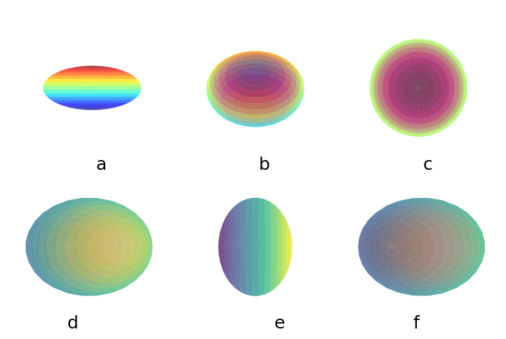
Fig. 4.4 An oblate spheroidal galaxy with \(a=b;\ c/a=0.6\) can be seen looking down the \(x\)-axis as the \(y-z\) plane (panel a), inclined by \(45^\circ\) (panel b), or inclined by \(90^\circ\) (panel c). The galaxy appears as an E0 (\(\beta/\alpha=1\)) when from the perspective in panel c, and resembles an E4 galaxy (\(\beta/\alpha=0.6\)) in panel b. A prolate spheroidal galaxy resembles an E0 galaxy in panel b, and an E4 in panel c. The python code below demonstrates how to create such a figure in python.#
import matplotlib.pyplot as plt
import numpy as np
from myst_nb import glue

def get_spheroid(a,b,c):
    u,v = np.mgrid[0:2*np.pi:30j, 0:np.pi:20j]
    x = a*np.cos(u)*np.sin(v)
    y = b*np.sin(u)*np.sin(v)
    z = c*np.cos(v)
    return x, y, z

fig = plt.figure(figsize=(12,4),dpi=150)
ax11 = fig.add_subplot(231, projection='3d')
ax12 = fig.add_subplot(232, projection='3d')
ax13 = fig.add_subplot(233, projection='3d')
ax21 = fig.add_subplot(234, projection='3d')
ax22 = fig.add_subplot(235, projection='3d')
ax23 = fig.add_subplot(236, projection='3d')
ax_list = [ax11,ax12,ax13,ax21,ax22,ax23]
ax_label = ['a','b','c','d','e','f']
fs = 'large'

for i in range(0,6):
    ax = ax_list[i]
    if i <3:
        x,y,z = get_spheroid(1,1,0.6)
        cmap=plt.cm.jet
        ax.view_init(45*i,0,0)
        ax.text(0,10,0,ax_label[i],color='k',fontsize=fs,horizontalalignment='center',transform=ax.transAxes)
    else:
        x,y,z = get_spheroid(1/0.6,1,1)
        cmap=plt.cm.viridis
        ax.view_init(45*i,0,90)
        ax.text(-i,0,8+i,ax_label[i],color='k',fontsize=fs,horizontalalignment='center',transform=ax.transAxes)
    ax.plot_surface(x,y,z,cmap=cmap,alpha=0.5)
    ax.set_aspect('equal')
    ax.set_axis_off()
    ax.set_xlim(-1,1)
    ax.set_ylim(-1,1)
    ax.set_zlim(-1,1)


fig.subplots_adjust(wspace=-0.75,hspace=0)
glue("spheroid_fig", fig, display=False);
The physical properties of elliptical galaxies span a wide range:
absolute \(B\) magnitudes range from \(-8\) (faintest) to \(-23\) (brightest)
masses (including both luminous and dark matter) vary from \(10^7\ M_\odot\) to more than \(10^{13}\ M_\odot\)
diameters can be \(0.1\ \rm kpc\) or as large as 100s of \(\rm kpc\).
The giant elliptical galaxies are some of the largest objects in the universe, while dwarf galaxies can be as small as a globular cluster. The lenticular galaxies have masses and luminosities comparable to the larger ellipticals. The dwarfs are the most numerous, even though the giant ellipticals and lenticulars are easier to observe. Typical examples of elliptical galaxies are shown in Fig. 4.5, along with an S0 and SB0.
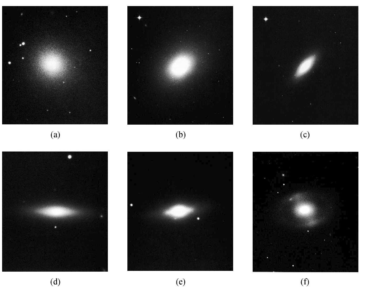
Fig. 4.5 Typical early-type galaxies (a) IC 4296 (E0), (b) NGC 4365 (E3), (c) NGC 4564 (E6), (d) NGC 4263 (E7), (e) NGC 4251 (S0), (f) NGC 4350 (RSB0). Image Credit: Sandage and Bedke (1994) from The Carnegie Atlas of Galaxies.#
Hubble subdivided the spiral sequences into Sa, Sab, Sb, Sbc, Sc, and SBa, SBab, SBb, SBbc, SBc. The galaxies with the
most prominent bulges (i.e., the largest bulge-to-disk luminosity ratios, \(L_{\rm bulge}/L_{\rm disk} \sim 0.3\)),
most tightly wound wound spiral arms (with pitch angles) of approximately \(6^\circ\)), and
the smoothest distribution of stars in the arms
are classified as Sa (or SBa), while Sc (or SBc) have
smaller bulge-to-disk ratios (\(L_{\rm bulge}/L_{\rm disk} \sim 0.05\)),
more loosely wound spiral arms (\(18^\circ\)), and
spiral arms that resolve into clumps of stars and H II regions. Examples of normal and barred spiral galaxies are shown in Figs. 4.6 and 4.7, respectively. M31 and NGC 891 are type Sb, whereas the Milky Way is probably a type SBbc.
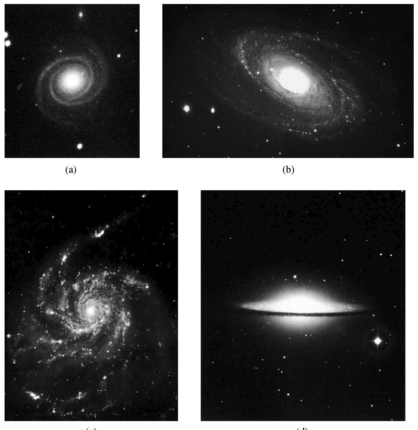
Fig. 4.6 Typical normal spiral galaxies. (a) NGC 7096 (Sa(r)I), (b) M81/NGC 3031 (Sb(r)I-II), (c) M101/NGC 5457/Pinwheel (Sc(s)I), (d) M104/NGC 4594/Sombrero (Sa/Sb) seen nearly edge on. Image Credit: Sandage and Bedke (1994) The Carnegie Atlas of Galaxies.#
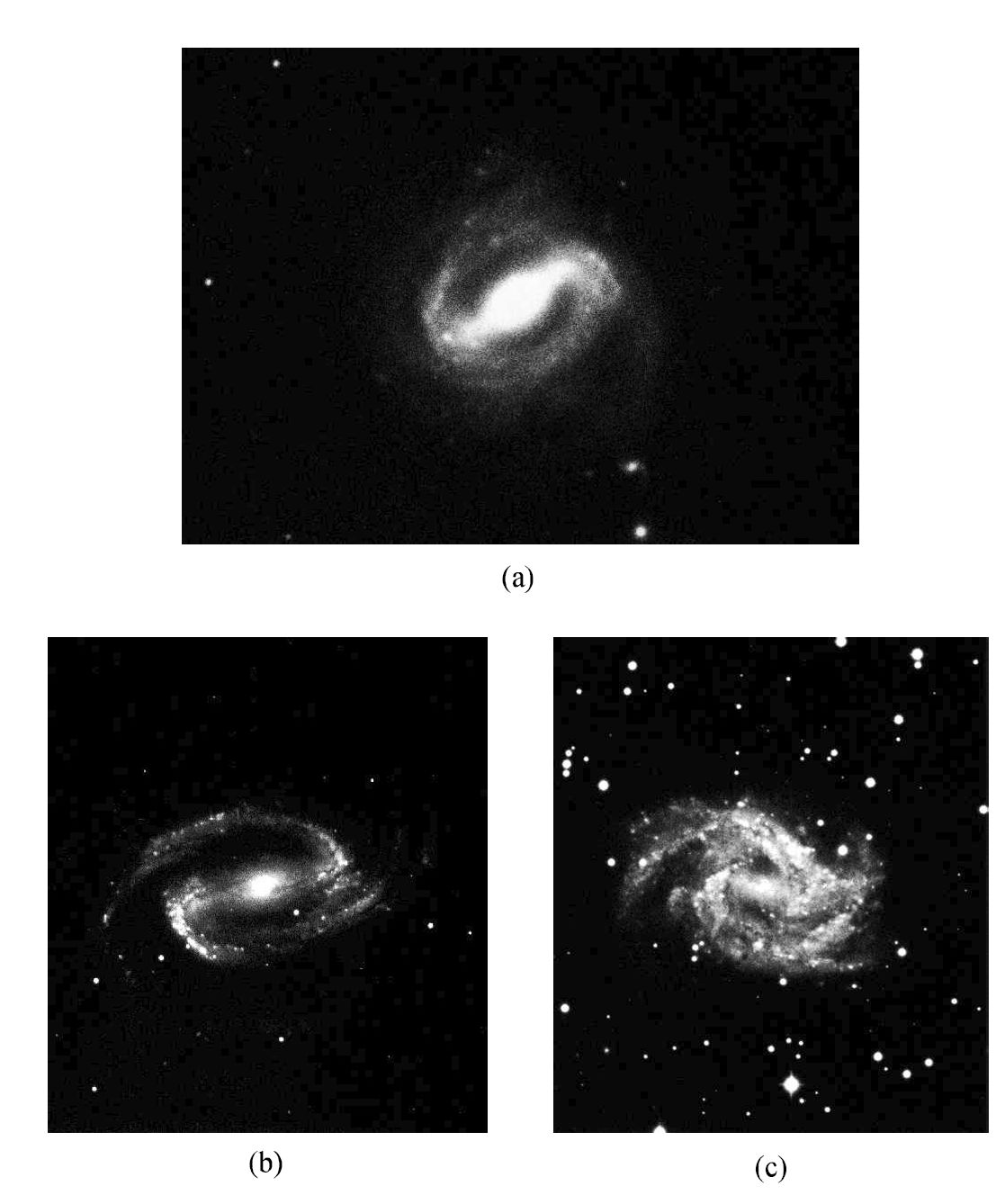
Fig. 4.7 Typical barred spiral galaxies. (a) NGC 175 (SBab(s)I-II), (b) NGC 1300 (SBb(r)I), (c) NGC 2525 (SBc(s)I). Image Credit: Sandage and Bedke (1994) from The Carnegie Atlas of Galaxies.#
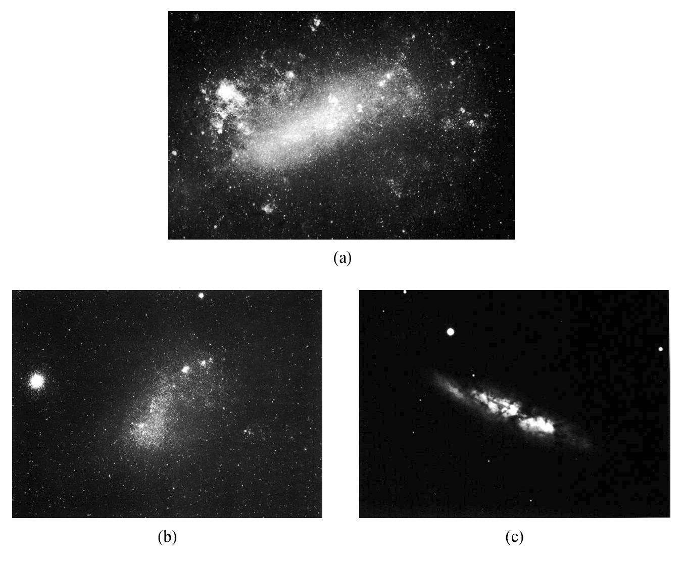
Fig. 4.8 Examples of irregular galaxies. (a) Large Magellanic Cloud (Irr I/SBmIII), (b) Small Magellanic Cloud (Irr I/ImIV-V), (c) M82/NGC 3034 (Irr II/Ir/Amorphous). Image Credit: Sandage and Bedke (1994) The Carnegie Atlas of Galaxies.#
Sa-Sc (SBa-SBc) galaxies tend to have much smaller variations in their physical parameters than do ellipticals. On average, spirals tend to be the largest galaxies in the universe, with
absolute \(B\) magnitudes from \(-16\) to less than \(-23\),
masses between \(10^9-10^{12}\ \rm M_\odot\), and
disk diameters of \(5-100\ \rm kpc\).
Hubble split the remaining category of irregulars into Irr I if there was at least some hint of an organized structure (e.g., spiral arms) and Irr II for the most extremely disorganized structures. The Large and Small Magellanic Clouds are examples of Irr I galaxies, while M82 (NGC 3034) is an example of an Irr II (see Fig. 4.8).
Irregular galaxies have a wide range of characteristics, although they tend not to be particularly large. They have
absolute \(B\) magnitudes from \(-13\) to \(-20\),
masses between \(10^8-10^{10}\ M_\odot\), and
diameters that range from \(1-10\ \rm kpc\).
Most irregulars also tend to have noticeable bars that are off-center.
Since Hubble’s publication of his tuning-fork diagram, astronomers have made modifications to his original classification scheme. Gerard de Vaucoulers suggested the elimination of the irregular classifications, Irr I and Irr II, in favor of the addition of other morphological classes later than Sc (or SBc). Those galaxies that were binned into Irr I have been designated Sd (SBd), Sm (SBm), or Im (where m stands for Magellanic type). The truly irregular galaxies are simply designated Ir (e.g., M82).
Sandage and Brucato further suggested that the Ir class should more appropriately be termed amorphous to indicate the lack of any organized structure. Spirals of Hubble-type Sd and later tend to be significantly smaller than earlier-type spirals, where they are sometimes referred to as dwarf spirals.
To make finer distinctions between normal and barred spirals, de Vaucouleurs had also suggested referring to normal spirals as SA rather than simply S. Intermediate types with weak bars are then characterized as SAB, and strongly barred galaxies are SB.
A further refinement to the system, the lenticular galaxies are also sometimes subdivided according to the amount of dust absorption in their disks. S03 galaxies have no discernable dust in their disks, while S03 galaxies have significant amounts of dust, and similarly for SB01 through SB03. The modern sequence from early ellipticals through normal late-type galaxies is
E0, E1, \(\ldots\), E7, S01, S02, S03, Sa, Sb, Sbc, Sc, Scd, Sd, Sm, Im, Ir.
A similar sequence exists for barred spirals.
Sydney van den Bergh introduced the luminosity class for spirals. The class ranges from I through IV, with I representing spirals with well-defined arms; galaxies with the least distinct arms are classified as V.
M31 is classified as SbI-II (intermediate between I and II),
the Milky Way is an SBbcI-II,
M101 is an ScI,
the Large Magellanic Cloud (LMC) is an SBmIII, and
the Small Magellanic Cloud (SMC) is an ImIV-V.
Except for the largest elliptical galaxies, the Milky Way and M31 are mong some of the largest and brightest galaxies in the universe.
Note
Despite its name, luminosity class does not necessarily correlate well with absolute magnitude.
Besides their striking arms, spirals also show an amazing array of more complex and subtle features. While some galaxies have spiral arms that can be followed nearly all the way into the center, others have arms that appear to terminate at the location of an inner ring. Special designations help further classify these systems.
M101 is a galaxy of the former type and is a labeled as an Sc(s)I, where (s) designates that the spiral can be traced to the center of the galaxy.
On the other hand, NGC 7096 and M81 are galaxies of the later type and are classified as Sa(r)I and Sb(r)I-II, respectively, where (r) indicates an inner ring.
Galaxies may also have outer rings (e.g., NGC 4340), which is designated as an RSB0, and the R prefix stands for outer ring.
4.2. Spiral and Irregular Galaxies#
Hubble’s classification scheme for late-type galaxies is very successful in organizing our study of these objects. The tightness of the spiral arms, the ability to resolve the arms into stars, the bulge-to-disk ratios, and the H II regions all correlate well with Hubble type. But so do a host of other physical parameters.
Tables 4.1 and 4.2 summarize the characteristics of early and late type spiral galaxies, also irregular galaxies. The spread in parameters can be quite large, but trends in the Hubble type are evident. If we compare an Sa galaxy with an Sc galaxy of comparable luminosity, the Sa will
be more massive (i.e., a larger \(M/L_B\)),
have a higher peak in its rotation curve (\(v_{\rm max}\)),
have a smaller mass fraction of gas and dust, and
contain a higher proportion of older, red stars.
Sa |
Sb |
Sc |
|
|---|---|---|---|
\(M_B\) |
\(-17\) to \(-23\) |
\(-17\) to \(-23\) |
\(-16\) to \(-22\) |
\(M\ (M_\odot)\) |
\(10^9-10^{12}\) |
\(10^9-10^{12}\) |
\(10^9-10^{12}\) |
\(\langle L_{\rm bulge}/L_{\rm total} \rangle_B\) |
\(0.3\) |
\(0.13\) |
\(0.05\) |
Diameter (\(D_{25}\ \rm kpc\)) |
\(5-100\) |
\(5-100\) |
\(5-100\) |
\(M/L_B\) (\(M_\odot/L_\odot\)) |
\(6.2 \pm 0.6\) |
\(4.5 \pm 0.4\) |
\(2.6 \pm 0.2\) |
\(\langle v_{\rm max} \rangle\ \rm (km/s)\) |
\(299\) |
\(222\) |
\(175\) |
\(v_{\rm max}\) range \(\rm (km/s)\) |
\(163-367\) |
\(144-330\) |
\(99-304\) |
pitch angle |
\({\sim}6^\circ\) |
\({\sim}12^\circ\) |
\({\sim}18^\circ\) |
\(\langle B-V \rangle\) color |
\(0.75\) |
\(0.64\) |
\(0.52\) |
\(\langle M_{\rm gas}/M_{\rm total} \rangle\) |
\(0.04\) |
\(0.08\) |
\(0.16\) |
\(\langle M_{\rm H_2}/M_{\rm H\ I} \rangle\) |
\(2.2\pm 0.6\) (Sab) |
\(1.8\pm 0.3\) |
\(0.73 \pm 0.13\) |
\(\langle S_N \rangle\) |
\(1.2\pm 0.2\) |
\(1.2\pm 0.2\) |
\(0.5 \pm 0.2\) |
Sd/Sm |
Im/Ir |
|
|---|---|---|
\(M_B\) |
\(-15\) to \(-20\) |
\(-13\) to \(-18\) |
\(M\ (M_\odot)\) |
\(10^8-10^{10}\) |
\(10^8-10^{10}\) |
Diameter (\(D_{25}\ \rm kpc\)) |
\(0.5-50\) |
\(0.5-50\) |
\(M/L_B\) (\(M_\odot/L_\odot\)) |
\({\sim}1\) |
\({\sim}1\) |
\(v_{\rm max}\) range \(\rm (km/s)\) |
\(80-120\) |
\(50-70\) |
\(\langle B-V \rangle\) color |
\(0.47\) |
\(0.37\) |
\(\langle M_{\rm gas}/M_{\rm total} \rangle\) |
\(0.25\) (Scd) |
\(0.5-0.9\) |
\(\langle M_{\rm H_2}/M_{\rm H\ I} \rangle\) |
\(0.03-0.3\) |
\({\sim}0\) |
\(\langle S_N \rangle\) |
\(0.5\pm 0.2\) |
\(0.5\pm 0.2\) |
4.2.1. The \(K\)-Correction#
There are problems with determining the brightness of a galaxy. As is the case with determining the absolute magnitudes for stars, calculating the absolute magnitudes of galaxies requires making corrections to their observed apparent magnitudes. These corrections must take properly account for the effects of extinction, both within the Milky Way and within the target galaxy.
Most galaxies are observed to have measurable redshifts. Some (or even most) of the light would normally fall within the wavelength band of interest (e.g., the B band) would be redshifted to longer wavelength regions. Accounting for this effect is known as the K-correction. The K-correction is most severe for very distant galaxies, where if this effect is ignored then the possible conclusions about the evolution of galaxies would be likely in error.
4.2.2. The Brightness of the Background Sky#
Another problem arises when making observations of faint galaxies (or when measuring their outermost regions) is the competition with the brightness of the background sky. The dimly glowing night sky has an average brightness of \(\mu_{\rm sky} = 22\ ({B\ \rm mag})/{\rm arcsec^2}\). Sources of this background light include
light pollution from nearby cities,
photochemical reactions in Earth’s upper atmosphere,
the zodiacal light,
unresolved stars in the Milky Way, and
unresolved galaxies.
In modern photometric studies using CCDs, the surface brightnesses of galaxies can be measured down to levels of \(29\ ({B\ \rm mag})/{\rm arcsec^2}\) or fainter. To accurately determine the light distribution of a galaxy at these extremely faint levels, it is necessary to subtract the contribution from the background sky.
4.2.3. Isophotes and the de Vaucouleurs Profile#
After a sky subtraction, it is possible to map contours of constant brightness, known as isophotes (i.e., lines of constant photon number). In specifying the “radius” of a galaxy, it is necessary to define the surface brightness of the isophote begin used to determine that radius.
No definite cutoff is known to exist in either the exponential distribution of the disk or the \(r^{1/4}\) distribution of the spheroid. One commonly used radius is the Holmberg radius \(r_H\), which is defined to be the projected length of the semimajor axis of an ellipsoid having an isophotal surface brightness of \(\mu_H = 26.5\ ({B\ \rm mag})/{\rm arcsec^2}\). A second standard radius in frequent use is the effective radius \(r_e\), which is the projected radius within which one-half of the galaxy’s light is emitted. The surface brightness level at \(r_e\) (designated as \(\mu_e\)) depends on the distribution of the surface brightness variations with radius.
For the bulges of spiral galaxies (and for large ellipticals), the surface brightness distribution follows an \(r^{1/4}\) law given by:
This is the \(r^{1/4}\) de Vaucouleurs profile written in units of \({\rm mag}/{\rm arcsec^2}\), rather than \(L_\odot/pc^2\).
Disks are frequently modeled with an exponential decay. However, the disk luminosity per unit area can be written in units of \({\rm mag}/{\rm arcsec^2}\) as
where \(h_r\) is the characteristic scale length of the disk along its midplane.
A generalized version of the \(r^{1/4}\) law is frequently used in which \(1/4\) is replaced by \(1/n\), which results in the generalized de Vaucouleurs profile and also known as the Sérsic profile. This has the form:
where \(\mu_e\), \(r_e\), and \(n\) are all free parameters used to obtain the best possible fit to the actual surface brightness profile.
4.2.4. The Rotation Curves of Galaxies#
While surface brightness profiles sample the distribution of luminous matter in a galaxy, they do not reveal the distribution of the galaxy’s dark matter. A galaxy’s rotation curve provides a direct means to determine the distribution of all matter (luminous and dark).
When rotation curves are compared with either luminosity (or Hubble type), a number of correlations are found.
With increasing luminosity in the \(B\) band \(L_B\), the rotation curves tend to rise more rapidly with distance from the center and peak at higher maximum velocities \(v_{\rm max}\).
For galaxies of equal \(B\)-band luminosities, spirals of an earlier type have larger maximum velocities.
Within a given Hubble type, galaxies that are more luminous have larger maximum velocities.
For a given maximum velocity \(v_{\rm max}\), the rotation curves tend to rise more rapidly with radius for galaxies of progressively earlier type.
The fact that galaxies of different Hubble types (and therefore different bulge-to-disk luminosity ratios) exhibit rotation curves that are very similar in form suggests that the shapes of their gravitational potential do not necessarily follow the distribution of luminous matter. This behavior is believed to be a signature of the existence of dark matter in these galaxies.
Although the maximum rotation velocity within the disk increases for earlier-type galaxies, a wide range in \(v_{\rm max}\) exists for each type. For typical samples of spirals of type Sc and earlier, the mean maximum rotation velocities \(v_{\rm max}\) are
\(299\ \rm km/s\) for Sa,
\(222\ \rm km/s\) for Sb, and
\(175\ \rm km/s\) for Sc,
while the ranges in values are given in Table 4.1. The maximum velocity for the Milky Way (believed to be an SBbc) is \(\simeq 250\ \rm km/s\), which is only slightly grater than the mean value of \(v_{\rm max}\) for Sb-type galaxies.
The corresponding maximum rotation velocities for irregular galaxies is significantly lower than it is for earlier-type spirals (typically ranging from \(50-70\ \rm km/s\)). This suggests that a minimum rotation speed of \({\sim}50-100\ \rm km/s\) may be necessary for the development of a well-organized spiral pattern. The slower velocities of Im-type galaxies imply that their values of the rotational angular momentum per unit mass are only about \(10\%\) of the solar neighborhood within the Milky Way.
4.2.5. The Tully-Fisher Relation#
A relationship exists between the luminosity of a spiral galaxy and its maximum rotation velocity. This correlation is now known as the Tully-Fisher relation, which uses the Doppler-broadening of emission lines of neutral hydrogen H I (i.e., the 21-cm line). When the 21-cm line is sampled across the entire galaxy at one time, it displays a double peak.
So much of the H I participates in the rotation at the maximum velocity, the flux density is greatest at this value. The double peak arises because
of the flat rotation curve of the galaxy, which generally has the highest rotational velocity in the flat part of the curve.
a portion of the disk is rotating toward or away from the observer, causing the line to be blueshifted or redshifted.
The average radial velocity of the galaxy relative to the observer is the midpoint value between the two peaks. The shift \(\Delta \lambda\) of a peak from its wavelength is given by,
The radial velocity \(v_r\) and inclination angle \(i\) between the observer’s line of sight and the direction perpendicular to the galactic plane affects our measurement of the shift. Note that \(i=90^\circ\) corresponds to viewing the galaxy edge-on.
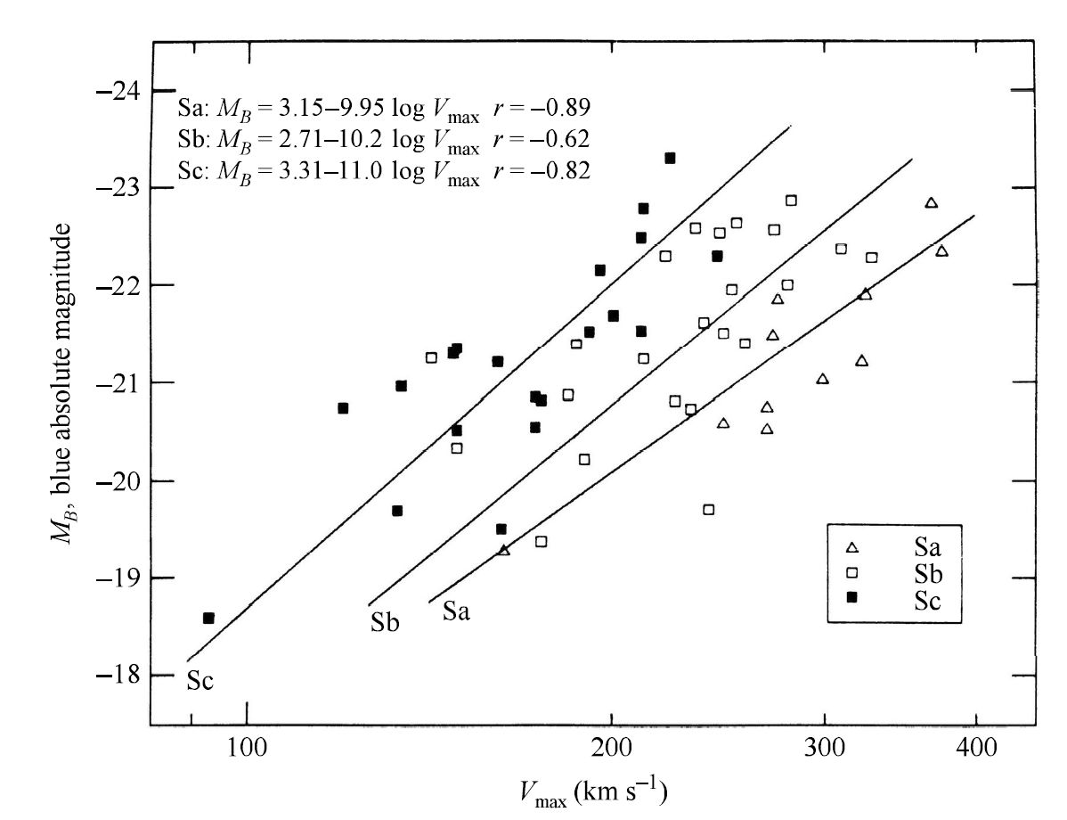
Fig. 4.9 The Tully-Fisher relation for early spiral galaxies. Image credit: Carroll & Ostlie (2007); Figure adapted from Rubin et al. (1985).#
Figure 4.9 shows the Tully-Fisher relation as \(M_B\) vs. \(v_{\rm max}\) for a sample of Sa, Sb, and Sc galaxies. There is a shift to lower values of \(v_{\rm max}\) for galaxies of later Hubble type but with a similar magnitude \(M_B\). When the data are fitted with linear relations that depend on Hubble type, we find that
The Tully-Fisher relation can be further refined and tightened if observations are made at infrared wavelengths. This offers two advantages:
Observing at dust-penetrating IR reduces extinction by a factor of 10.
The IR light come from primarily late-type giant stars that are good tracers of the galaxy’s overall luminous matter distribution; the \(B\) band tends to emphasize you, hot stars in regions of recent star formation.
One expression of the Tully Fisher relation in the IR \(H\) wavelength band (\(1.66\ \mu \rm m\); Pierce and Tully (1992) is:
where the measure of the rotation of the galaxy \(W_R^i\) is defined as
The parameter \(W_{20}\) depends on the velocity difference between the blueshifted and redshifted emission in the \(H\) band when the intensity of the emission is \(20\%\) of its blue and red peak values. The other parameter \(W_{\rm rand}\) is a measure of the random velocities superimposed on the observed velocities due to noncircular orbital motions of the galaxy. The inclination angle \(i\) is between the plane of the galaxy and the observer’s line-of-sight. An example of the \(H\)-band Tully-Fisher relation for galaxies in three clusters is shown in Figure 4.10.
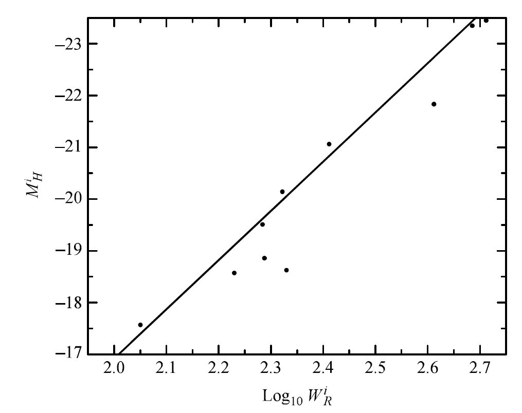
Fig. 4.10 The Tully-Fisher relation in the IR \(H\)-band. The data are for galaxies in the Local, Scupltor, and M81 groups of galaxies. Image credit: Carroll & Ostlie (2007); Data from Pierce and Tully (1992).#
Although the exact form of the Tully-Fisher relation depends on the distribution of mass within galaxies (as well as variations in their mass-to-light ratios), we can still gain some insight into its origin. Spiral galaxies have nearly flat rotation curves beyond a few \(\rm kpc\). Evaluating this for the entire galaxy (\(r\rightarrow R\) and \(M_r\rightarrow M\)) results in
where the maximum rotation speed \(v_{\rm max}\) is equated with the flat portion of the rotation curve.
If the mass-to-light ratio has the same value for all spirals (\(M/L \equiv 1/C_{\rm ML}\), where \(C_{\rm ML}\) is a constant), then
Through a crude assumption that all spirals have the same surface brightness at their centers, then \(L/R^2 \equiv C_{\rm SB}\) (\(C_{\rm SB}\) is another constant). Eliminating \(R\) from the expression for the luminosity, we obtain
where \(C\) incorporates the other constants. The absolute magnitude comes from,
Although the additive (zero-point) constant remains unevaluated, this simple argument nearly reproduces the leading coefficients, the slopes of the \(B\)-band Tully-Fisher relation for early spirals (Sa, Sb, and Sc), and the slope of the collective relationship in the \(H\) band.
4.2.6. Radius-Luminosity Relation#
Another important pattern also emerges in the data of early-type spiral galaxies: Radius increases with increasing luminosity, independent of Hubble type. At the disk radius \(R_{25}\) corresponding to a surface-brightness level of \(25\ B\ \text{mag/arcsec}^2\), the data are well represented by the linear relationship
where \(R_{25}\) is measured in \(\rm kpc\).
4.2.7. Colors and the Abundance of Gas and Dust#
The trend in \(M/L_B\) suggests that Sc galaxies tend to have a greater fraction of massive main sequence stars relative to earlier spirals. If this is the case, we should also expect Sc galaxies to be bluer than Sa and Sb galaxies, which is just what is observed. The mean values of \(B-V\) (color index) decrease with later Hubble types:
0.75 for Sa,
0.64 for Sb, and
0.52 for Sc.
For successively later-type galaxies, progressively greater portions of the overall light from spirals is emitted in bluer wavelength regions, implying an increasingly greater fraction of younger, more massive, main-sequence stars.
Irregulars tend to be the bluest of all galaxies represented by the Hubble sequence, with characteristic \(B-V \sim 0.4\). Furthermore, Ir galaxies often get bluer toward their centers, rather than redder as is the case for early-type spirals. This suggests that irregulars are still actively manufacturing stars in their central regions. For instance, the LMC and SMC still appear to be making blue globular clusters in their disks.
Blue main-sequence stars are short-lived, they must have formed relatively recently. Presumably an abundant supply of gas and dust exists in Sc galaxies from which these stars can be produced. Based on the analysis of 21-cm radiation, \(\rm H\alpha\) emission, and \(\rm CO\) emission, we find that the mass fraction of gas relative to the total mass interior to \(R_{25}\) increases steadily from Sa to Sc and later.
The relative amounts of atomic and molecular hydrogen also change with Hubble type. This observation has been interpreted as implying that Sa galaxies are somewhat more centrally condensed, containing correspondingly deeper gravitational wells in which gas can collect and combine to form molecules. Overall the amount of molecular hydrogen in spirals can range from \(5 \times 10^{10}\ M_\odot\) for the most massive galaxies to as little as \(10^6\ M_\odot\) for dwarf spirals. The mass of dust is characteristically \(150-600\) times lower than the mass of gas in the ISM.
4.2.8. Metallicity and Color Gradients of Spirals#
Not only is there a dependence of color on Hubble type, but individual spiral galaxies also exhibit color gradients with their bulges generally being redder than their disks. This arises for two reasons: metallicity gradients and star formation activity.
The average number of electrons per atom is larger for metal-rich stars than for metal-poor stars. Since ionization and the orbital transitions of electrons contribute to the opacity in stellar photospheres, the opacity in metal rich stars is greater. Because it is more difficult light generated in the interior to escape from a star with a higher opacity photosphere, the star will tend to “puff up” (increase in radius), with a corresponding decrease in effective temperature. A high-opacity star will be redder than a lower opacity star, all else being equal.
The redness of bulges argues for those regions begin more metal-rich than are the portions of disk farther from the center, as is the case in our own Galaxy. Within the Milky Way, metallicity gradients have been measured at Galactocentric radii between \(4-14\ \rm kpc\) with values of \(d[He/H]/dr = -0.01 \pm 0.008\ \rm dex/kpc\), \(d[O/H]/dr = -0.07 \pm 0.015\ \rm dex/kpc\), and \(d[Fe/H]/dr = -0.01\ \text{to } -0.05\ \rm dex/kpc\).
Note
The unit \(\rm dex\) refers to the logarithmic nature of the metallicity term in the gradient.
Star formation (the second major cause of color gradients) implies that the disks of spiral galaxies are more actively involved in star-making than are their bulges. This is consistent with the distribution of gas and dust in the galaxies. The spheroidal components usually contain much less gas and have correspondingly lower star formation rates than their disks. Since disks are able to produce young, hot, blue stars at a greater rate, the spheroids appear relatively redder and a color gradient is established.
Color gradients have been observed within the spheroids of spiral galaxies as well (e.g., NGC 7814). The galaxies’ spheroidal components become bluer with increasing radius. This is also the case for the Milky Way, with more metal-rich, redder globular clusters orbiting closer to the Galactic center.
Observations indicate that metallicity correlates with the absolute magnitude of galaxies; [Fe/H] and [O/H] both increase with \(M_B\). Apparently chemical enrichment was somehow more efficient in luminous, massive galaxies. Composition enrichment histories and gradients have significant implications for galaxy formation theories.
4.2.9. X-ray Luminosity#
The X-ray luminosities of galaxies also provide some information concerning their evolution. In spirals, luminosities in the wavelength region sampled by the Einstein observatory (with photon energies of \(0.2-3.5\ \rm keV\)) typically range from \(L_X = 10^{31}-10^{34}\ \rm W\). A surprisingly tight correlation exists between X-ray and \(B\)-band luminosities (\(L_x/L_B \simeq 10^{-7}\)), which has been interpreted as implying that the X-rays are due to a class of objects that constitutes an approximately constant fraction of the population of all objects in spirals. The suspected sources are X-ray binaries. It is probable that supernova remnants also contribute to the X-ray emission.
4.2.10. Supermassive Black Holes#
Observations of stellar and gas motions near the centers of some spirals suggest the presence of supermassive black holes. For instance, near the center of M31, the \(M/L\) exceeds \(35\ M_\odot/L_\odot\), which indicates a large amount of nonluminous matter confined to a small region. Rotational-velocity measurements can be used to estimate the dynamical mass of the central black hole of M31 in the same way it was done for Sgr \(\rm A^*\) in the Galactic center.
A precise determination on kinematic studies of the triple nucleus of M31 gives a mass of \(1.4^{+0.9}_{-0.3} \times 10^8\ M_\odot\) for the supermassive black hole. Another (less precise) method of determining the mass of a central supermassive black hole uses the velocity dispersion to obtain a mass estimate via the virial theorem. The time-averaged kinetic and potential energies of stars in the galaxy’s central region are related by
where \(I\) is the region’s moment of inertia. If the galaxy is in equilibrium, then \(\langle d^2 I/ dt^2 \rangle = 0\), resulting in the usual statement of the virial theorem,
For a large number of stars, the central bulge will look the same (in a statistical sense) at any time, and the time-averaging can be dropped. So for \(N\) stars,
For simplicity, we restrict our attention to a spherical cluster of radius \(R\) with \(N\) stars, each of mass \(m\), so the total mass of the bulge is \(M = Nm\). Dividing the above expression by \(N\) produces
Astronomers actually measure the radial component of the velocity vector (i.e., a galaxy is too far away to allow for detection of proper motions). Also, an astronomer is just as likely to see a star moving in the radial direction as in either of the transverse directions. With the brackets denoting an average value,
so
where \(\sigma_r\) is the dispersion in the radial velocity. Inserting into our result from the virial theorem (Eq. (4.10)), and using the approximate potential energy of a spherical distribution of total mass \(M\) and radius \(R\), leads to
Using \(M = Nm\) and solving for the mass gives
where the mass obtained is called the virial mass.
To determine an accurate value for the mass, an appropriate choice of \(R\) must be made. As the observations move farther from the black hole, contributions to the total mass increase from surrounding stars and gas. The radius \(R\) must be chosen to be within the black hole’s “sphere of influence.”
Exercise 4.1
The central radial-velocity dispersion of M32 (a companion galaxy to M31) is approximately \(162\ \rm km/s\).
Estimate a virial mass for the central black hole of M32.
The virial mass can be computed using Eq. (4.11) assuming a radius \(R \sim 0.1^{\prime\prime}\) (or approximately \(0.4\ \rm pc\) of the center). There is a total mass of roughly
A more accurate estimate (based on the rotation curve) gives a value between \(1.5 \times 10^6\ \rm M_\odot\) and \(5\times 10^6\ M_\odot\)
from scipy.constants import G, parsec

sigma_r = 162e3 #velocity dispersion in m/s
R_influence = 0.4*parsec #radius of influence in m
M_sun = 1.99e30

M_virial = 5*R_influence*sigma_r**2/G/M_sun #virial mass in M_sun
print("The virial mass is approximately %1.0e M_odot." % M_virial)
The virial mass is approximately 1e+07 M_odot.
Central supermassive black holes are not restricted to late-type galaxies. Observations made with the Hubble Space Telescope (HST) show that the giant elliptical galaxy M87 (NGC 4476) also contains a \(3.2 \pm 0.9 \times 10^9\ M_\odot\) black hole. HST was able to resolve a disk of material within M87 that has rotational speeds reaching \(550\ \rm km/s\), where the disk itself is orbiting an central region no larger than our Solar System.
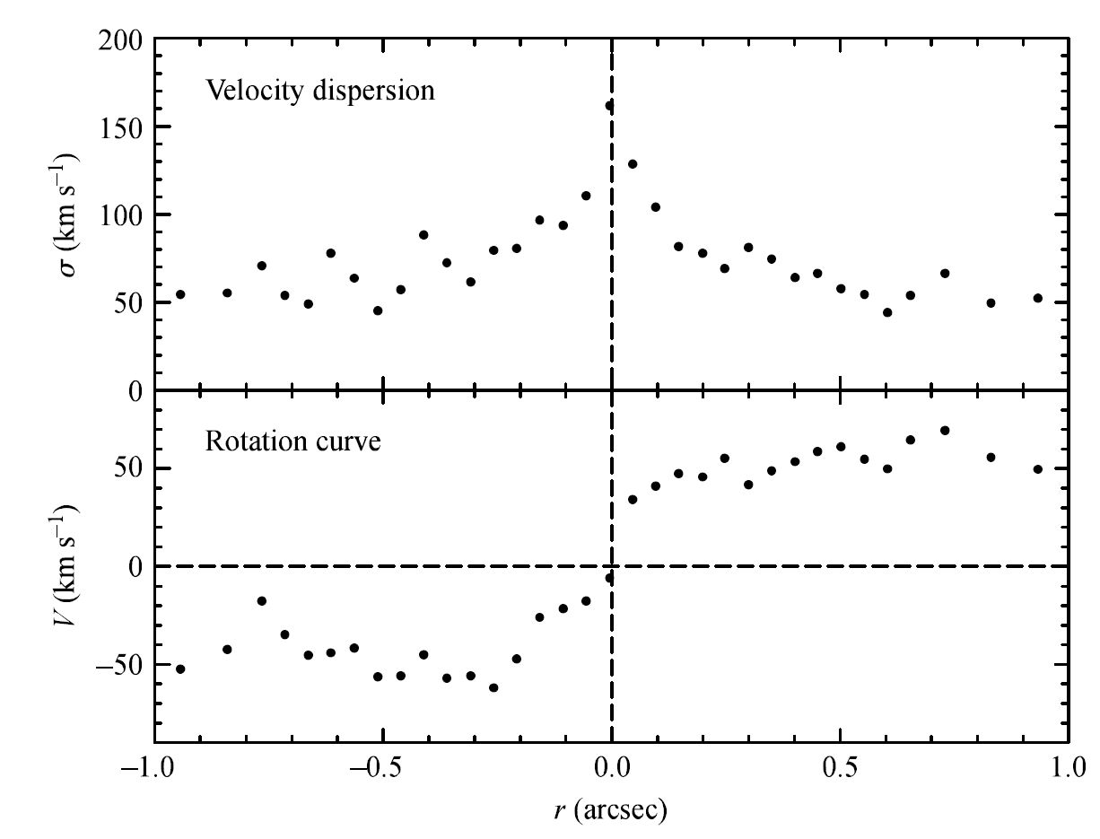
Fig. 4.11 The stellar velocity dispersion and rotational velocities of stars near the center of M32. Given the distance to M32 of \(770\ \rm kpc\), \(1^{\prime\prime}\) corresponds to a linear distance from the center of \(3.7\ \rm pc\). Image Credit: Carroll & Ostlie (2007); Data taken from Joseph et al. (2001).#
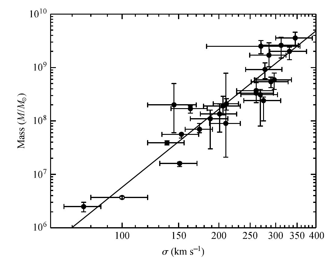
Fig. 4.12 The relationship between the mass of a galaxy’s supermassive black hole and the velocity dispersion \(\sigma\) of the galaxy’s spheroid. The dataset includes elliptical, lenticular, and spiral galaxies. Image Credit: Carroll & Ostlie (2007); data taken from Ferrarese and Ford (2005). The open symbol represents the Milky Way with mass data from Ghez et al. (2005).#
As the number of known supermassive black holes increased, it became possible to look for relationships between the black holes and their host galaxies. A useful correlation exist between the mass of the supermassive black hole in a galaxy’s center and the velocity dispersion of the stars within the galaxy. The relationship is given by the best fit power law (see Fig. 4.12),
where \(\sigma\) is the velocity dispersion (in \(\rm km/s\)). The fitted coefficients are \(\alpha = (1.66 \pm 0.24) \times 10^8\ M_\odot\), \(\beta = 4.86 \pm 0.43\), and \(\sigma_o = 200\ \rm km/s\).
The velocity dispersion is measured for the stellar population near the black hole. Correlations between the mass of the supermassive black holes and other bulk galaxy parameters (e.g., luminosity of the bulge) have been uncovered. A fundamental link may exist between the formation of the central supermassive black hole in a galaxy and the overall formation of the galaxy itself, but the precise details are still to be determined.
4.2.11. Specific Frequency of Globular Clusters#
The abundance of globular clusters in late-type galaxies has important implications for theories of galactic formation and evolution. Galaxies that are more spheroidally dominant (i.e., earlier Hubble types) were more efficient at forming globular clusters during their histories. Virtually all galaxies appear to contain some globular clusters, but the number of clusters within a galaxy seems to increase with total galaxy luminosity and with progressively earlier Hubble type.
The globular cluster counts are usually normalized to a standard absolute magnitude for the parent galaxy of \(M_V = -15\ \rm mag\) to compare cluster systems among Hubble types more directly. If \(N_t\) is the total number of globular clusters in a galaxy, then the specific frequency of globular clusters are
where \(L_V\) is the galaxy’s luminosity and \(L_{15}\) is the reference luminosity corresponding to an absolute value of \(M_V = -15\ \rm mag\).
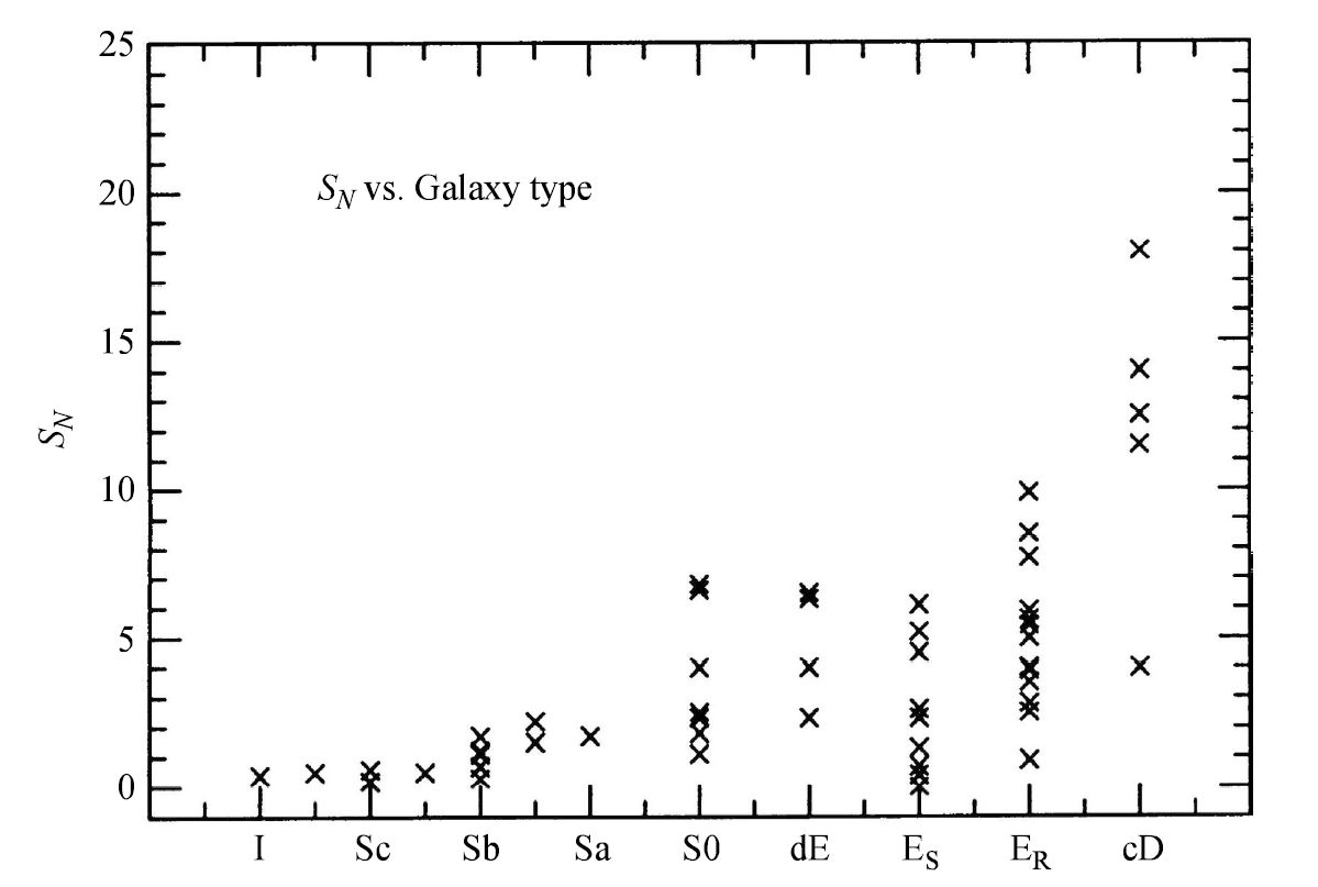
Fig. 4.13 The association of the specific frequency of globular clusters with Hubble type. \(\rm cD\) galaxies are the large elliptical galaxies in the universe; \(\rm dE\) refers to dwarf ellipticals. Image Credit: Carroll & Ostlie (2007); figure adapted from Harris (1991).#
Figure 4.13 shows for \(\rm Sc\) galaxies and later, the average value of \(S_N\) is in the range of \(0.5 \pm 0.2\), while for \(\rm Sa\) and \(\rm Sb\) galaxies, \(\langle S_N \rangle\) increases to \(1.2 \pm 0.2\). \(\langle S_N \rangle\) is even larger for elliptical galaxies, which means that they have more clusters per unit luminosity than do spirals.
4.3. Spiral Structure#
Galaxies exhibit a rich variety of spiral structure, which vary in
the number of arms and how tightly wound they are,
degree of smoothness in the distribution of stars and gas
surface brightness, and
the existence (or lack) of bars.
The most majestic spiral galaxies (known as grand-design spirals) usually have two very symmetric and well-defined arms.
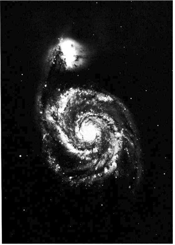
Fig. 4.14 The Whirlpool galaxy M51 (NGC 5194) is an Sbc(s)I-II grand-design spiral located in the constellation Canes Venatici. Also visible is its companion NGC 5195. Image Credit: Carroll & Ostlie (2007); Image from Sandage and Bedke (1994) The Carnegie Atlas of Galaxies.#
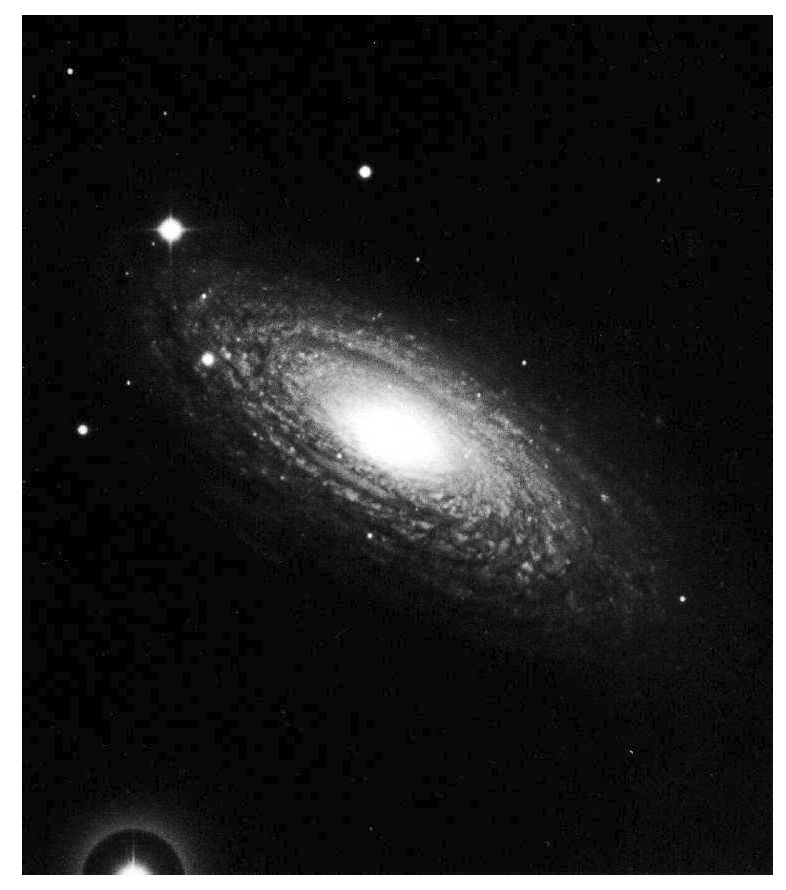
Fig. 4.15 The Sb galaxy NGC 2841 is an example of a flocculent spiral. Image Credit: Carroll & Ostlie (2007); Image from Sandage and Bedke (1994) The Carnegie Atlas of Galaxies.#
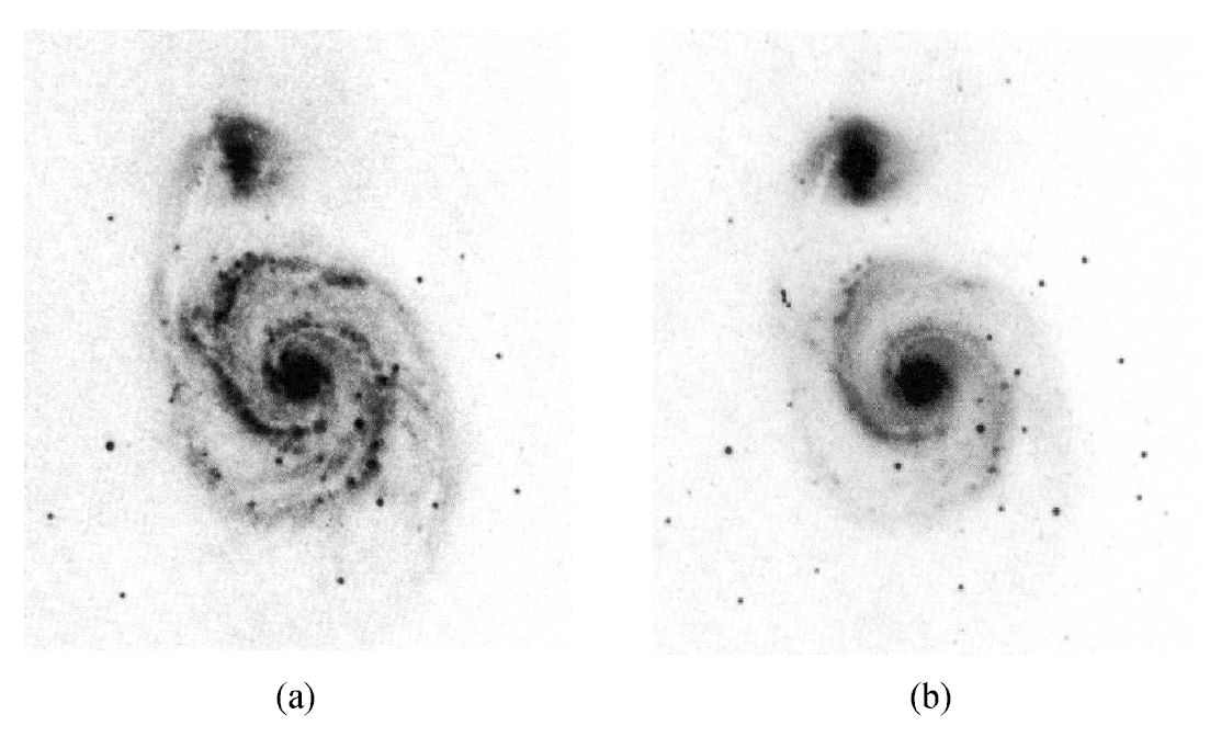
Fig. 4.16 M51 seen in (a) blue light and (b) red light. Image Credit: Carroll & Ostlie (2007); Figure from Elmegreen (1981).#
However, not all spirals are grand designs with two distinct arms. For instance, M101 has four arms, and NGC 2841 has a series of partial arm fragments. Galaxies like NGC 2841, which do not possess well-defined spiral arms that are traceable over a significant angular distance are called flocculent spirals. Only \({\sim}10\%\) of all spirals are considered grand-design galaxies, another \(60\%\) are multiple-arm galaxies, and the remaining \(30\%\) are flocculent galaxies.
The optical images of spiral galaxies are dominated by their arms because very luminous O and B main-sequence stars and H II regions are found preferentially in the arms. Massive OB stars are short-lived objects relative to the characteristic rotation period of a galaxy, where spiral structure corresponds to regions of active star formation.
Careful inspection of the spiral galaxies reveals that dust bands are also evident in the spiral arms. Notice that the dust bands tend to reside on the inner (concave) edges of the arms. Observation of 21-cm H I emission indicates that gas clouds are also more prevalent near the inner edges of the arms.
When spiral galaxies are observed in red light, the arms become much broader and less pronounced. Although they still remain detectable. Observations at red wavelengths emphasize the emission of long-lived, lower-mass main-sequence stars and red giants, which implies that the bulk of the disk is dominated by older stars. Despite the dominance of lower-mass stars between the spiral arms, observations show that there is still an increase in the number density of older stars within the spiral arms.
4.3.1. Trailing and Leading Spiral Arms#
The general appearance of spiral galaxies suggests that their arms are trailing, where the tips of the arms point in the opposite direction relative to the direction of rotation. Distinguishing between trailing and leading arms (along the direction of rotation) requires determination of the orientation of the plane of the galaxy relative to our line-of-sight so that radial velocity measurements can be unambiguously interpreted in terms of the direction of the galaxy rotation.
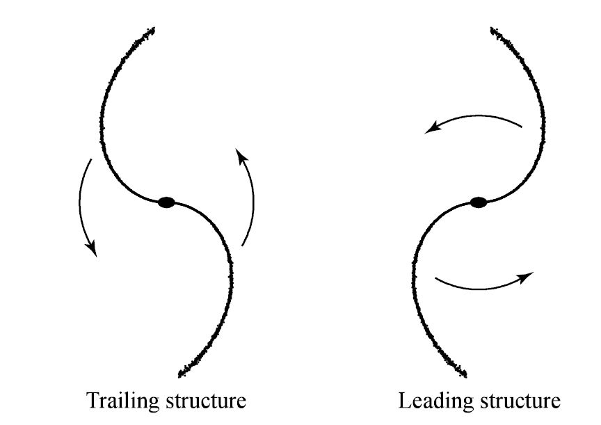
Fig. 4.17 Trailing and leading spiral arm structures. Image Credit: Carroll & Ostlie (2007).#
In almost all cases, where such a clear determination can be made, it does appear that spiral arms are trailing. In NGC 4622, two arms are going one way and another arm is winding in the opposite direction; at least one of these arms must be leading. M31 (Andromeda) also has one tightly wound leading arm. In each case, it is likely that the leading spiral arm is produced through a tidal encounter with a retrograde-moving object, where M32 is the likely culprit in the case of M31.
4.3.2. The Winding Problem#
Spiral galaxies are common within the universe, so it is natural to ask what causes spiral structure, and whether spiral arms are long-lived (i.e., lifetimes comparable to the age of the galaxy) or transient.
One problem arises when the nature of the spiral structure is considered: material arms composed of a fixed set of identifiable stars and gas clouds would necessarily “wind up” on a timescale that is short compared to the age of the galaxy.
The winding problem can be understood by considering a set of stars that are originally along a straight line, but at varying distances from the center of the galaxy. Since the disk of a spiral galaxy rotates differentially (except very near the center), the outer stars will require more time to complete one orbit that will stars with smaller orbital radii (recall Kepler’s 3rd law). This effect will lead to a natural generation of trailing spiral arms. However, after a few orbits, the spirals will become too tightly wound to be observed. Another mechanism is needed to explain persistent spiral structure.
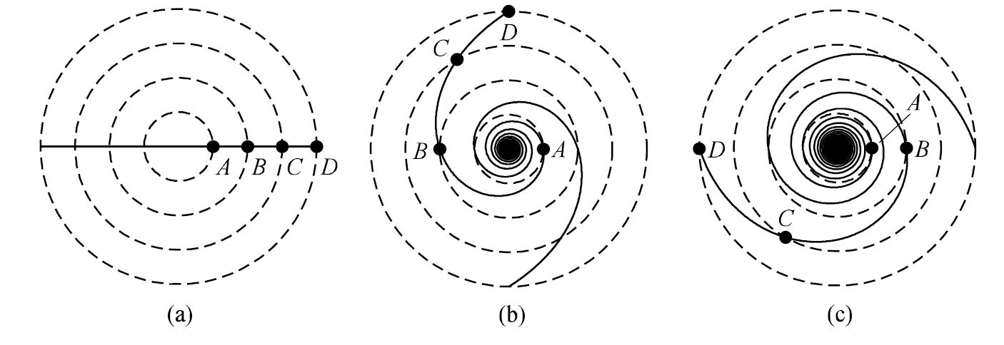
Fig. 4.18 The winding problem for material arms. The arms become progressively more tightly wound as time goes on. A flat rotation curve is assumed with \(R_B = 2R_A\), \(R_C = 3R_A\), and \(R_D= 4R_A\). (a) The star start out in a line at time \(t=0\). (b) After star A has completed one orbit. (c) After star A has completed two orbits. Image Credit: Carroll & Ostlie (2007).#
4.3.3. The Lin-Shu Density Wave Theory#
In the mid-1960s, C.C. Lin and Frank Shu proposed that spiral structure arises because of the presence of long-lived quasistatic density waves. Density waves consist of regions in the galactic disk where the mass density is greater than average, perhaps by \(10-20\%\). Stars, dust, and gas clouds move through the density waves during their orbits around the galactic center, much like cars slowly working their way through a traffic jam on a highway.
Lin and Shu suggested that when the galaxy is viewed in a noninertial reference frame that is rotating with a specific angular speed \(\Omega_{gp}\) known as the global pattern speed, the spiral wave pattern appears to be stationary. This is simply an effect of the reference frame (e.g., the stroboscopic effect) and does not imply that the motions of the stars are also stationary.
Stars near the center of the galaxy can have orbital periods that are shorter than the density wave pattern (i.e., \(\Omega > \Omega_{gp}\)) and so they will overtake the spiral arm, move through it, and continue on until they encounter the next arm. Stars sufficiently far from the center of the galaxy will be moving more slowly than the density wave pattern and will be over taken by it (\(\Omega < \Omega_{gp}\)).
The corotation radius \(R_c\) is a specific distance from the center, where the density wave pattern is static. The stars with \(R<R_c\) will appear to pass through the arms moving in one direction, while stars with \(R>R_c\) will appear to moving in an opposite sense.
The Lin-Shu hypothesis helps explain many of the observations concerning spiral structure. For instance,
the ordering of H I clouds and dust bands on the inner (trailing) edges of spiral arms),
the existence of young, massive stars and H II regions throughout the arms, and
an abundance of old, red stars in the remainder of the disk.
As dust and gas clouds within the corotation radius overtake a density wave, they are compressed by the effects of the increase in local mass density. This causes some of the clouds to satisfy the Jeans criterion and begin to collapse, resulting in the formation of new stars. This process takes some time (\({\sim}10^5\ \rm yr\) for a \(15\ M_\odot\) star), the appearance of new stars will occur within the arm slightly “downstream” from dust and gas clouds at the edge of the wave.
The birth of the brightest and bluest new stars (e.g., massive O and B stars) will result in the creation of H II regions as the UV ionizing radiation moves through the interstellar medium (ISM). Massive stars have relatively short lifetimes, which means they will die before they can move entirely out of the density wave in which they were born.
Less massive, redder stars will be able to live much longer (some much longer than the current age of the galaxy) and so will continue through the density wave and become distributed throughout the disk. Local maxima in the number density of red dwarfs within spiral arms are due to the presence of the density wave during a subsequent passage, which causes the stars to collect a the bottom of the wave’s gravitational potential well. The same scenario could also occur on the outer (leading) edges of spiral arms outside the corotation radius. However, it is likely that less dust and gas will be found in these outer regions of the galaxy.
In principle, the density wave theory suggests a solution to the winding problem. The problem arose because we considered material arms. If the stars are allowed to pass through a quasistatic density wave (i.e., a buoy on the ocean), then the problem has been changed to one of establishing and maintaining the wave of enhanced density. There has been a lot of research into density waves since the Lin-Shu hypothesis was proposed, even within the context of planet or satellite formation in the Solar System.
4.3.4. Small-amplitude Orbital Perturbations#
Let’s explore how the orbital motions of individual stars about the galactic center can result in spiral-shaped regions of enhanced density according to the Lin-Shu hypothesis. Consider the general motion of a star (or gas cloud) in an axially symmetric gravitational field that is also symmetric about the galactic midplane (i.e., a pancake or disk). We are assuming that density waves make an insignificant contribution to the gravitational field, which may not be valid in all spiral galaxies. However, this assumption does simplify the analysis considerably.
The position of a star at some general point above the galactic plane can be written using the unit vectors of a cylindrical coordinate system, or
where cylindrical coordinates has three unit vectors: \(\hat{\mathbf{e}}_R\), \(\hat{\mathbf{e}}_\phi\), and \(\hat{\mathbf{e}}_z\). To convert between rectangular and cylindrical coordinates, we have
For a star of mass \(M\), Newton’s second law of motion in cylindrical coordinates is
where \(\mathbf{F}_g\) is the gravitational force on the star, and the \(\phi\)-dependence is neglected due to the assumption of axial symmetry. Replacing the force with the negative of the gradient of the gravitationa potential energy, yields
Dividing both sides by the star’s mass, writing the result in terms of the gravitational potential \(\Phi \equiv U/M\), and noting that \(U = -GMm/R\) is independent of \(\phi\) gives
Since we are producing a model using cylindrical coordinates, let’s compare our acceleration to the general solution of an acceleration in cylindrical coordinates (see the video below for a derivation).
The general solution is as follows
where the dots represent time derivatives (\(d/dt\)). Comparing the general solution to our model (Eq. (4.15)), we see that
Because we have assumed axial symmetry, there is no component of the force vector in the \(\hat{\mathbf{e}}_\phi\) direction and no component of torque along the \(z\)-axis. Therefore the \(z\) component of the star’s orbital angular momentum \(L_z\) must be constant since \(\tau_z = dL_z/dt = 0\) (i.e., conservation of angular momentum). We can define
The constant \(J_z\) represents the \(z\) component of the orbital angular momentum per unit mass of the star. This allows us to define the following relations:
Inserting into the radial equation in Eq. (4.17) gives
To simplify the expression, we define an effective gravitational potential that incorporates a term representing the star’s kinetic energy per unit mass associated with the azimuthal motion (\(v_\phi = R\dot{\phi} = J_z/R\)):
Now the radial and vertical equations of motion can be written as
using the \(z\) acceleration from Eq. (4.17).
To solve these equations for the motion of the star through the galaxy, we must first determine the behavior of the effective potential \(\Phi_{\rm eff}\). It would be helpful to know where the minima are located, since the star should attempt to settle into an orbit of minimum possible energy. In other words, we want to solve
Given our assumption that the gravitational potential is symmetric about the midplane, the second condition is satisfied at \(z = 0\) because \(\Phi\) (and \(\Phi_{\rm eff}\)) must be either a local maximum or minimum there. Since \(\Phi <0\) and is assumed to be identically zero at infinity, it is necessary that \(\Phi_{\rm eff}\) be a minimum at \(z=0\)
The physical significance of the minimum in \(\Phi_{\rm eff}\) with respect to \(R\) is realized using \(J_z\) as a constant of the star’s motion,
for some radius \(R_m\) in the galaxy’s midplane (\(z=0\)). This gives
Since \(J_z = Rv_\phi\), the right-hand side is just
which is the centripetal acceleration for perfectly circular motion. The left-hand side of (4.22) is the radial component of the gradient of the true gravitational potential. The last expression is the familiar equation for perfectly circular motion,
and the minimum value for the \(\Phi_{\rm eff}\) occurs when the star is executing perfectly circular orbital motion in the midplane of the spiral galaxy.
To understand the first-order effects of deviations from the minimum value of \(\Phi_{\rm eff}\), we will expand \(\Phi_{\rm eff}\) about its minimum position \((R_m,0)\) by means of a 2D Taylor series (see this video by 3Blue1Brown).
Letting \(\rho \equiv R - R_m\) and using the subscript \(m\) to indicate that the leading constant and partial derivatives are begin evaluated at the minimum position, we obtain
The first term on the right-hand side is the constant minimum value in \(\Phi_{\rm eff}\), and the two first-derivative terms are identically zero (recall we used them to identify the extrema). The mixed-partial derivative is also identically zero because of the symmetry of \(\Phi_{\rm eff}\) about the \(z=0\) plane.
Let’s define the constants
and neglect the remaining higher-order terms. Then the effective gravitational potential becomes
Notice that the non-constant terms resemble the potential energy of a classical harmonic oscillator (i.e., \(kx^2/2\)). Since \(\ddot{\rho} = \ddot{R}\), we arrive at two of the three first-order expansions for the equations of motion about a perfectly circular orbit in the galaxy’s midplane:
which are the familiar differential equations of simple harmonic motion. Therefore we can use the known solution to the harmonic oscillator to give
where \(\kappa\) is called the epicycle frequency, \(R_m\) is the radius of the energy-minimum circular orbit, and \(A_R\) is the amplitude of the radial oscillation.
Similarly, we can describe the motion of a star above and below the Galactic midplane with \(\nu\) being the vertical oscillation frequency. The star’s position along the \(z\)-axis is given by
where \(A_z\) is the amplitude of the oscillation in the \(z\) direction and \(\zeta\) is a general phase shift between \(\rho(t)\) and \(z(t)\).
We now have two expressions that describe the motion of a star about an equilibrium position (\(R=R_m;\ z=0\)) that is moving in a circular orbit. To complete our description of the approximate motion of the star, consider its azimuthal angular speed, which is given by
But \(R(t) = R_m + \rho(t) = R_m\left( 1+ \frac{\rho(t)}{R_m} \right)\). Assuming \(\rho(t) \ll R_m\) and using the binomial expansion theorem to first order,
Substituting the expression for \(\rho(t)\) from the epicycle frequency (Eq. (4.27)) into the approximation above and integrating with respect to time, we find that
where \(\Omega \equiv J_z/R_m^2\). The first two terms in this expression correspond to the perfectly circular orbit traced out by the equilibrium point, moving at a constant angular speed \(\Omega\). The last term represents the oscillation of the star about the equilibrium point in the \(\phi\) direction.
Defining \(\chi(t) = \left[ \phi(t) - (\phi_o + \Omega t) \right]R_m\) to be the difference in azimuthal position between the star and the equilibrium point. Then, we have
The three equations (Eqs. (4.27), (4.28), and (4.29)) we derived represent the motions of the star in the \(R\), \(z\), and \(\phi\) coordinates, respectively, about an equilibrium position that is moving in a perfect circle around the center of the galaxy and the galactic midplane.
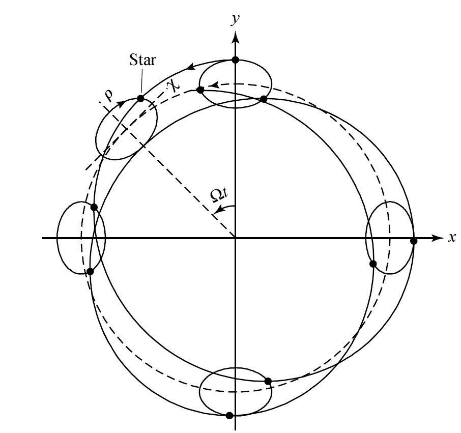
Fig. 4.19 In an inertial reference frame a star’s orbital motion in the galactic midplane (solid line) forms a nonclosing rosette pattern. In the first-order approximation, the motion can be imagined as being the combination of a retrograde orbit about an epicycle and the prograde orbit of the center of the epicycle about a perfect circle (dashed line). The dimensions of the epicycle have been exaggerated by a factor of 5 to illustrate the effect. Image Credit: Carroll & Ostlie (2007).#
The star’s orbit is not closed in an inertial reference frame, but produces a rosette pattern. However, the star can be imagined as being located on an epicycle, with the center of the epicycle corresponding to the equilibrium position. As the star moves in a retrograde direction about the epicycle, it is carried alternately closer to and farther from the galactic center. The epicycle is also oval in shape and has an axial ratio that is given by the ratios of the amplitudes of the oscillations in \(\chi\) and \(\rho\), or \(2\Omega/\kappa\). The \((\chi,\ \rho)\) coordinate system of the epicycle rotates about the galaxy’s center with the angular speed \(\Omega\) (i.e. the angular speed of the equilibrium point).
Note
This model bears a strong resemblance to the epicycle-deferent models of planetary motion devised by Hipparchus and Ptolemy. In those ancient planetary models, the epicycles were assumed to be perfectly circular.
Exercise 4.2
Our Sun is moving relative to a perfectly circular motion called the Local Standard of Rest (LSR), as reflected in the Sun’s peculiar solar motion. The Sun must have a nonzero epicycle frequency. Information about the radial component of the Sun’s peculiar motion is also contained in the Oort constants (\(A\) and \(B\)), since they involve derivatives of the Sun’s orbital speed \(\Theta_o\) with respect to the Galactocentric radius \(R_o\).
Values of the Oort constants for the Sun: \(A = 14.8\ \rm km/s/kpc\) and \(B = -12.4\ \rm km/s/kpc\).
Determine the epicycle frequency \(\kappa_o\) in terms of the Oort constants and identify how it compares with the orbital angular frequency \(\Omega_o\).
For the condition for perfectly circular motion, we have
which arises because the angular momentum per unit mass is \(J_z = R_o \Theta_o\) at the solar Galactocentric distance. Substituting into the expression for the square of the epicycle frequency (Eq. (4.27)) and making use of effective potential \(\Phi_{\rm eff}\), we find that the solar epicycle frequency is
Rewriting this in terms of the Oort constants (see link above)
Using the values for the Oort constants, the epicycle frequency for our Sun is \(\kappa_o = 36.7\ \rm km/s/kpc = 1.2 \times 10^{-15}\ rad/s\). This value for the epicycle frequency corresponds to an oscillation period of \(P = 2\pi/\kappa_o = 170\ \rm Myr\).
The ratio of the Sun’s epicycle frequency to its orbital angular speed (or orbital frequency) \(\Omega_o = \Theta_o/R_o = A-B\) is
which indicates that the Sun executes 1.35 epicycle oscillations for every orbit around the Galactic center.
The axial ratio of the Sun’s epicycle is given by
4.3.5. Closed Orbits in Noninertial Frames#
The number of oscillation per orbit about the galaxy’s center is equal to the ratio of the star’s epicycle frequency to its orbital angular speed. If the ratio \(\kappa/\Omega\) is a ratio of integers, the orbit is closed.
However, most stellar orbits are not closed and a rosette pattern results. But in a noninertial reference frame that is rotating with a local angular pattern speed \(\Omega_{lp} = \Omega\) relative to the inertial frame, the star’s path would appear to be very simple tracing out a closed orbit that is retrograde and centered at a distance \(R_m\) from the galaxy’s center (see Fig. 3 of Quarles et al. (2020) for an example using the circular restricted three body problem (CRTBP)). Such a reference frame corresponds to that epicycle’s own coordinate system in which the equilibrium point is stationary and the closed path simply traces the epicycle itself.
To obtain a closed orbit in a noninertial frame, we need no necessarily choose an angular pattern speed that equals the unperturbed orbital angular speed \(\Omega\). Instead, we could choose to have the star complete \(n\) orbits as seen in the rotating frame while executing \(m\) epicycle oscillations (where \(n\) and \(m\) are non-zero integers), after which time the star would be back at its starting point. We could choose \(m(\Omega -\Omega_{lp}) = n\kappa\), or
Note that this is a local pattern speed, so \(\Omega_{lp}\) is a function of \(R\). In principle, there are an infinite number of local pattern speeds at each \(R\), only a small number of value of \(n\) and \(m\) produce substantial enhancements in mass density.
Note
This problem is analogous to situations encountered within the Solar System. For example, the orbital resonances of Saturn’s moons (primarily Mimas) with particles in the planet’s ring system produce gaps in the rings. In addition, small integer ratios between Jupiter’s orbital period and the orbital periods of asteroids result in either increases or decreases in the number of asteroids having certain orbital radii.
Now imagine a large number of stars at various distances R from the center of a spiral galaxy, all observed in a reference frame rotating with the global angular pattern speed \(\Omega_{gp}\). If we consider the case \((n,\ m) = (1,\ 2)\) and if the local pattern speed \(\Omega_{lp} = \Omega(R) - \kappa(R)/2\) is a constant for all values of \(R\), then we can set \(\Omega_{gp} = \Omega_{lp}\).
Seen from the noninertial frame, the resulting orbital patterns could be nested with their major axes aligned. The structure that results bears a significant resemblance to the bars present in roughly two-thirds of all spiral galaxies. We could also orient each successive oval-shaped orbit so that its major axis is rotated slightly relative to the one immediately interior to it. in this example, the result is a trailing two-armed grand-design spiral wave pattern. Twisting the ovals in the opposite sense would result in a leading two-armed spiral. The two-armed spiral M51 is an example of a trailing-arm (\(n=1,\ m=2)\) pattern structure, while the four-armed spiral M101 is an (\(n=1,\ m=4)\) system. Patterns with \(m=2\) are the most common type of density wave structure.
It is important to remember that the individual stars are following their own orbits in an inertial reference frame and that these orbits appear only as simplified oval shapes in a reference frame that is rotating with the local angular pattern speed. Even in the rotating frame, the stars themselves are still moving along the oval orbits. Only the spiral pattern appears to be static in that frame. In the nonrotating inertial frame the spiral pattern will appear to move with an angular speed of \(\Omega_{gp}\). It is the “traffic jam” of stars becoming packed together where their oval orbits approach one another that leads to the density waves.
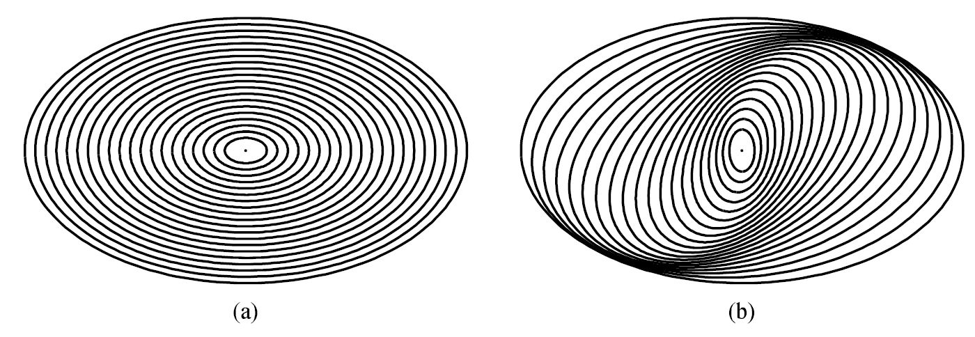
Fig. 4.20 (a) Nested oval orbits with aligned major axes, as seen in a reference frame rotation with the global angular pattern speed \((n=1,\ m=2)\), or \(\Omega_{gp} = \Omega-\kappa/2\). The result is a bar-like structure. (b) Each oval is rotated relative to the orbit immediately interior to it. The result is a two-armed grand-design spiral density wave. Image Credit: Carroll & Ostlie (2007).#
The stability of the structures shown in Fig. 4.20 depends crucially on whether \(\Omega_{lp} = \Omega(R) - \kappa(R)/2\) is actually independent of \(R\) (i.e., whether there is an appropriate global value of \(\Omega_{gp}\)). Figure 4.21 shows curves of \(\Omega(R) - n\kappa(R)/m\) with several ratios of \(n/m\) for one model of our Galaxy. Notice that \(\Omega -\kappa/2\) is nearly flat over a wide range of values for \(R\).
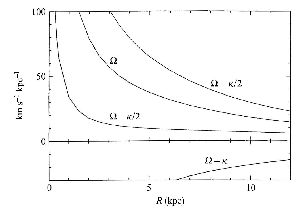
Fig. 4.21 The Bahcall-Soneira model of our Galaxy has been used to construct the functions \(\Omega_{lp} = \Omega -n\kappa/m\) for various ratios of \(n/m\). Image Credit: Carroll & Ostlie (2007). Figure adapted from Binney and Tremaine: Galactic Dynamics.#
The same general behavior is exhibited by a large number of spiral galaxies and probably accounts for the prevalence of two-armed spirals. Of course, \(\Omega -\kappa/2\) is not exactly constant with respect to the galactocentric radius, so some drifting of epicycle orbits relative to one another does occur, leading once again to a winding problem. In this case, the winding occurs for density waves rather than material waves, and because the relative drift is slower, the winding takes about five times longer to develop.
4.3.6. Nonlinear Effects in Density Wave Theory#
A complete understanding of density waves has not yet been fully realized. For instance, various effects not considered in the simple model may play important roles (e.g, nonlinear (higher-order) terms in \(\Phi_{\rm eff}\)). The waves themselves alter the gravitational potential in which they originate so that azimuthal symmetry breaks down.
One important driving mechanism in a number of grand-design spirals (including M51) is the presence of a companion galaxy that triggers spiral structure through tidal interactions. Although a detailed discussion is not presented here, techniques for studying spiral density waves have much in common with the theoretical procedures used to investigate stellar pulsation. Both linear and nonlinear models have been employed in the investigation of spiral structure.
4.3.7. Numerical \(N\)-Body Simulations#
An important example of a nonlinear \(N\)-body simulation of a rotating disk is one that was calculated in an early work by Frank Hohl (in 1971). In that calculation, \(10^5\) stars were initially placed in axisymmetric orbits, but as the simulation progressed, Hohl’s model proved to very unstable against the development of the \(m=2\) pattern, and a two-armed spiral density wave developed (\(t=2\)). As the simulation continued, the disk became “hot”, which meant that the velocity dispersion of its stars became large relative to their orbital velocities, and the spiral structure dissipated. A bar instability persisted throughout the rest of the simulation, and the final structure bears a strong resemblance to an SB0 galaxy.
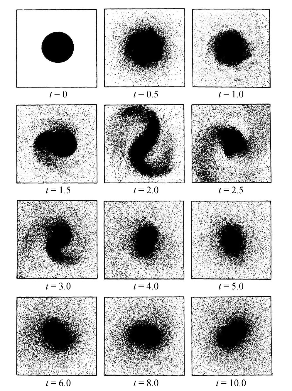
Fig. 4.22 An early study of a rotating disk with an \(N\)-body simulation using \(10^5\) stars. The disk began with complete axial symmetry and quickly developed an \(m=2\) mode instability. Eventually the disk “heated up,” destroyig the spiral arms but leaving a long-lived bar. Image Credit: Carroll & Ostlie (2007). Figure from Hohl (1971).#
Such bar instabilities have proved themselves to be common features in \(N\)-body calculations. Apparently a rotating disk is highly susceptible to a bar-mode instability. There is strong support for the idea that bar modes are favored in real galaxies as well, since roughly 2/3 of all disk galaxies do exhibit bar-like structures in their centers.
Hohl’s work suggest one possible means of stabilizing disks against various mode instabilities: the presence of high-velocity dispersions of its stars. In his original simulations, Hohl’s bar heated the disk, destroying the \(m=2\) trailing-arm mode. Tidal interactions and/or mergers may also play important roles in heating the disks of spiral galaxies.
In modern \(N\)-body simulations, models have included the effects of highly centralized masses (e.g., the gravitational influence of SMBHs). The inclusion of sufficiently condensed and massive central mass concentrations can weaken (and even destroy) the bar instability. Most studies find that a mas son the order of a few percent of the galaxy’s disk is required to affect the bar.
4.3.8. Stochastic, Self-Propagating Star Formation#
Many of the galaxies observed in the universe are flocculent spirals. It could be that these objects are composed of a linear combination of several stable density perturbations, which is somewhat reminiscent of modes in stellar oscillations. Especially if there is sufficient patchiness in the ISM to give the appearance of less well-defined spirals. Alternatively it may be that an entirely different mechanism is responsible for the spiral structure seen in these galaxies.
M. W. Mueller and William David Arnett proposed a theory of spiral structure for flocculent spirals known as stochastic, self-propagating star formation (SSPSF). In their theory, they imagine spiral structure arising from outbursts of star formation that propagate across the galaxy. When one region of the galaxy undergoes a star formation episode, its most massive stars will age rapidly, producing core-collapse supernovae. The supernovae shock waves will travel through the ISM, triggering the collapse of other gas clouds in nearby regions, where further star formation will occur, allowing the process to continue.
The above scheme has been compared to a forest fire, with the flames jumping from tree to tree. Spiral structure arises when the differential rotation of the galaxy draws these newly “lit” regions into trailing arms. Although SSPSF has been successful in producing flocculent spiral structure in computer simulations, it is unable to account for the transitions from dust lanes to OB stars to red stars across the spiral arms of grand-design spirals. It may well be that we will need both of these theories (and perhaps others) to understand the abundance of spiral structure found throughout the universe.
4.4. Elliptical Galaxies#
Although Hubble type correlates well with a wide variety of physical parameters for late-type galaxies, the Hubble-type designation for early galaxies (which is based solely on apparent ellipticity) has shown itself irrelevant in terms of trying to categorize other characteristics. As a result, subtype distinctions are made for ellipticals that are independent of the ellipticity and focus instead on other morphological features (e.g., size, absolute magnitude, and surface brightness of the image).
Ellipticals have come to be seen as remarkably diverse and complex. Some of this complexity may arise (at least in part) from strong environmental evolution, possibly involving tidal interactions or mergers with neighboring galaxies.
4.4.1. Morphological Classes#
Today a number of separate morphological classes are commonly used to distinguish among the elliptical galaxies.
cD galaxies are immense, rare, bright objects that sometimes measure nearly \(1\ \rm Mpc\) across and are usually found only near the centers of large, dense clusters of galaxies.
Their absolute \(B\) magnitudes range from less than \(-22\) mag to \(-25\) mag, and they have masses between \(10^{13}-10^{14}\ M_\odot\).
cD galaxies are characterized by having central regions with high surface brightnesses (\(\mu = 18\ B\ \text{mag/arcsec}^2\)).
They may also possess tens of thousands of globular clusters, with typical specific frequencies $S_N = 15.
These galaxies are known to have very high mass-to-light ratios, sometimes exceeding \(750\ M_\odot/L_\odot\), implying large quantities of dark matter.
Normal elliptical galaxies are centrally condensed objects with relatively high surface brightnesses. They include the giant ellipticals (gE), intermediate-luminosity ellipticals (E), and compact ellipticals (cE).
The absolute \(B\) magnitudes of normal ellipticals range from \(-15\) to \(-23\), masses between \(10^8-10^{13}\ M_\odot\), diameters are on the order of \(1-200\ \rm kpc\), mass-to-light ratios from \(7-100\ M_\odot/L_\odot\), and specific frequencies range \(S_N = 1-10\).
Lenticular galaxies (S0 and SB0) are often grouped with normal ellipticals.
Dwarf elliptical galaxies (dE) have surface brightnesses that tend to much lower than those of a compact elliptical (cE) of the same absolute magnitude.
The absolute \(B\) magnitudes fall between \(-13\) and \(-19\), they have typical masses of \(10^7-10^9\ M_\odot\), and their diameters are on the order of \(1-10\ \rm kpc\).
Their metallicities also tend to be lower than for normal ellipticals (E).
The average specific frequency of globular clusters is \(\langle S_N \rangle = 4.8 \pm 1.0\), which is still higher than for spirals.
Dwarf spheroidal galaxies (dSph) are extremely low-luminosity, low-surface brightness objects that have been detected only in the vicinity of the Milky Way.
Their absolute \(B\) magnitudes are only \(-8\) to \(-15\) mag, their masses are roughly \(10^7-10^8\ M_\odot\), and their diameters are between \(0.1-0.5\ \rm kpc\).
Blue compact dwarf galaxies (BCD) are small galaxies that are unusually blue with color indices ranging from \(\langle B-V \rangle = 0.0\ \text{to } 0.3\). This corresponds to main-sequence stars of spectral class A, which indicates that these galaxies are undergoing particularly vigorous star formation.
They have absolute \(B\) magnitudes from \(-14\) to \(-17\), masses on the order of \(10^9\ M_\odot\), and diameters of less than \(3\ \rm kpc\).
They have a large abundance of gas, with \(M_{\rm H\ I} = 10^8\ M_\odot\) and \(M_{\rm H\ II}=10^6\ M_\odot\) constituting roughly \(15-20\%\) of the entire mass of the galaxy.
They also have correspondingly low mass-to-light ratios; in an extreme case, ESO400-G43 has \(M/L_B = 0.1\) despite the dominance of dark matter at large radii.
4.4.2. Dust and Gas#
The low gravitational binding energy of dE and DSph galaxies means that it would be very difficult for these galaxies to retain a significant amount of gas, where this also bears out in observations.
dSph galaxies are virtually devoid of gas.
Both dE and dSph galaxies are not actively forming stars today.
They both have very low metallicities, with values similar to those found in globular clusters.
These systems may have lost most of their gas via supernova-driven mass loss or by ram-pressure stripping as the galaxies passed through the gas found in galaxy clusters.
For many years, it was thought that all elliptical galaxies had been largely stripped of any dust or gas that had not yet formed into stars, or that star formation had proceeded very efficiently during the earliest history of these galaxies, thereby depleting all the available gas. However, gas and dust are present within most normal elliptical galaxies, although at somewhat diminished levels relative to spirals.
The hydrogen gas that is present in E/S0 galaxies is usually evident in several forms.
A \(10^7\ \rm K\) X-ray emitting hot-gas component of \(10^8-10^{10}\ M_\odot\) makes up the majority of all the gas that is present in a typical E/S0 galaxy. The possible heating mechanisms include supernovae and stellar winds.
A warm-gas component (\(10^4-10^5\ \rm M_\odot\ \text{at } 10^4\ K\)), observable in \(\rm H\alpha\) is also present in the form of H II regions.
A cold-gas component composed of H I regions (\(10^7-10^9\ M_\odot\ \text{at }{\sim}100\ K\)) is detectable at 21 cm.
\(\rm CO\) emission studies indicate that \(10^7-10^9\ M_\odot\) of molecular hydrogen can be found in early-type galaxies as well.
Astronomers have discovered that perhaps \(50\%\) off all elliptical galaxies contain appreciable amounts of dust, with typical masses in the range of \(10^5-10^6\ M_\odot\). There exist dust lanes that are essentially randomly oriented with respect to their parent galaxy’s optical-light axes. Frequently, the dust is even found to be counter-rotating relative to the rotation direction of other (stellar) components. Apparently, much of this gas was acquired after the initial formation of the galaxy.
4.4.3. Metallicity and Color Gradients#
The metallicity of elliptical galaxies is well-correlated with luminosity, which means that brighter galaxies have a higher overall metal content. The metallicity and color gradients (changes in a parameter with radius) also exist in ellipticals, as with spiral galaxies. The central regions of E-type galaxies are redder and more metal-rich than are regions at larger radii.
This trend can be expressed in terms of the gradient of the mass fraction of metals found in the distribution of stars; typically \(d\log_{10} Z/d\log_{10} r \approx -0.13\). The same is also true for lenticular galaxies. The disks of S0 galaxies are bluer than their bulges, as is the case for galaxies of later Hubble types. Any successful theory of galaxy formation must incorporate the available observations concerning chemical enrichment.
4.4.4. The Faber-Jackson Relation#
One relationship that dE, dSph, normal E, and the bulges of spiral galaxies all have in common is the correlation between their central radial-velocity dispersion \(\sigma\) and \(M_B\). To see why the relation arises, we start with the virial theorem for the central dispersion of a spherically symmetric mass distribution (Eq. (4.11)). In that case, we made an approximation that a mass \(M\) was uniformly distributed throughout a volume of radius \(R\). Now, if we further assume that the mass-to-light ratio is essentially constant for all galaxies and that their average surface brightnesses are equal, we arrive at
where \(\sigma_r\) is replaced to \(\sigma_o\) to signify the central value for the radial velocity dispersion is being assumed. This relationship was first identified by Sandra Faber and Robert Jackson and is now referred to as the Faber-Jackson relation. Expressing the luminosity in solar units (i.e., \(L_\odot\)), taking the logarithm of both sides of the equation, and writing \(\log_{10}(L/L_\odot)\) as the difference in \(M_B\) values, we find the linear relationship between \(\log_{10}\sigma_o\) and \(M_B\), which is given as,
4.4.5. The Fundamental Plane#
There is considerable scatter in the data used to define the Faber-Jackson relation (Bender et al. (1992)). This is further reflected in the fact that the slope of the best-fit line through the data differs slightly from the expected result of the Faber-Jackson relation. Apparently \(L \propto \sigma_o^4\) isn’t strictly true, which isn’t surprising given the number of assumptions. Depending on the sample used, \(L \propto \sigma_o^\alpha\), withe \(3< \alpha < 5\).
Astronomers have introduced a second parameter into the expression to find a tighter fit to the data, using the effective radius \(r_e\). One representation of this fit is
Here galaxies are visualized as residing on a 2D “surface” in the 3D “space” represented by the coordinates \(L\), \(\sigma_o\), and \(r_e\). The above equation is known as the fundamental plane that combines the contributions of a galaxy’s gravitational well (i.e., velocity dispersion \(\sigma_o\)) with its radius and luminosity. Alternatively, the fundamental plane can be written in terms of the effective surface brightness of a galaxy at its effective radius:
The fundamental plane appears to represent the whole family of elliptical galaxies and may imply something about the formation of these systems.
4.4.6. The Effects of Rotation#
Parameterizations (e.g., the fundamental plane) do a much better job of classifying ellipticals than Hubble’s original scheme based on ellipticity. Then, what is the source of a galaxy’s shape? It is evident that most ellipticals are not purely oblate or prolate rotators with two axes, but are triaxial, which means that there is no single preferred axis of rotation. Evidence exists in the:
randomness of dust lanes found in at lest \(50\%\) of all ellipticals,
observations of counter-rotating stellar cores in as many as \(25\%\) of larger ellipticals.
It appears that (in at least some cases) material in the form of gas, dust, globular clusters, or dwarf galaxies has been captured sometime since the galaxy’s formation.
When the rotational velocities of elliptical galaxies are measured, we find that the more luminous ones have mean rotational velocities that are much less than their velocity dispersions, which implies that the shapes of these galaxies are not due to rotation. Instead, their shapes are caused by anisotropic velocity dispersion of stars in the galaxies.
Note
An anisotropic velocity distribution is one for which 1-2 directions of motion are preferred, rather than being completely random in all three dimensions, as in an isotropic distribution.
In one particularly extreme case, NGC 1600 (the luminous E4 galaxy) has \(M_B = -22.87\), \(v_{\rm rot} = 1.9 \pm 2.3\ \rm km/s\), and \(v_{\rm rot}/\sigma < 0.013\); it has no uniques axis of rotation that is statistically significant.
If the ellipticity \(\epsilon\) of a galaxy were due to its being an ideal, oblate rotator with an isotropic stellar velocity distribution, then it follows
For NGC 1600, this means that if its ellipticity of \(\epsilon = 0.4\) were due to pure rotation, then \(v_{\rm rot}/\sigma\) should be approximately 0.8. The ratio of the observed velocity distribution to the one expected from an isotropic distribution is defined as
The \(\left(v/\sigma\right)^*\) for NGC 1600 is less than 0.016. Although the distinction is somewhat arbitrary, a galaxy is considered to primarily rotationally supported if \(\left(v/\sigma\right)^* > 0.7\).
Bright E- and gE-type galaxies have typical values of \(\langle \left(v/\sigma\right)^* \rangle \approx 0.4\) and are pressure-supported, which means that there shapes are due primarily to random stellar motions. The diffuse, faint dE-type galaxies have predominantly anisotropic velocity dispersions and are also pressure-supported. Galaxies for which \(-18 > M_B > -20.5\ \rm mag\) have \(\langle \left(v/\sigma\right)^* \rangle \approx 0.9,\) which implies that they are largely rotationally supported. The bulges of spiral galaxies tend to be rotationally supported.
4.4.7. Correlations with Boxiness or Diskiness#
Ralf Bender, Jean-Luc Nieto, and their collaborators proposed (in 1988) that many of the characteristics of elliptical galaxies can be understood in terms of the degree of boxiness or diskiness that there isophotal surfaces exhibit. The shape of an isophotal contour is written in polar coordinates (as a Fourier series) of the form
which depends on the contour radius \(a\) and the angle \(\theta\) that is measured counterclockwise from the major axis of the ellipsoid. The terms of the expansion represent:
the shape of a perfect circle in the first term,
the amount of ellipticity in the second term, and
the degree of boxiness in the third term.
If \(a_4 < 0\), the surface tends toward a “boxy” appearance, and if \(a_4 > 0\), the surface tends towards being “disky” (see Fig. 4.23 and the associated python code). Typically, \(|a_4/a_o| \sim 0.01,\) with deviations from perfect ellipses routinely measured to an accuracy of \({\sim}0.5\%\).
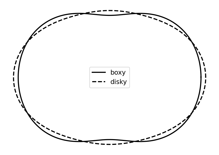
Fig. 4.23 Two examples of galaxies with \(\epsilon = 0.2\). \(|a_4/a_o|\) has been set to the rather large value of 0.03 to illustrate the effect. The “boxy” galaxy (solid line) has a \(a_4/a_o < 0\), while the “disky” galaxy has a \(a_4/a_o > 0\).#
import matplotlib.pyplot as plt
import numpy as np
from myst_nb import glue

def isophotal_contour(a0,a2,a4):
    theta = np.arange(0,2*np.pi+0.01,0.01)
    a = a0 + a2*np.cos(2*theta) + a4*np.cos(4*theta)
    return a*np.cos(theta), a*np.sin(theta)

a0 = 1
a2 = 0.2 #ellipticity

fig = plt.figure(figsize=(7,5),dpi=150)
ax = fig.add_subplot(111)

x_boxy, y_boxy = isophotal_contour(a0,a2,-0.03*a0)
x_disky, y_disky = isophotal_contour(a0,a2,0.03*a0)
ax.plot(x_boxy,y_boxy,'k-',lw=2,label='boxy')
ax.plot(x_disky,y_disky,'k--',lw=2,label='disky')

ax.legend(loc='best',fontsize='large')
ax.axis('off')

glue("boxy_disky_fig", fig, display=False);
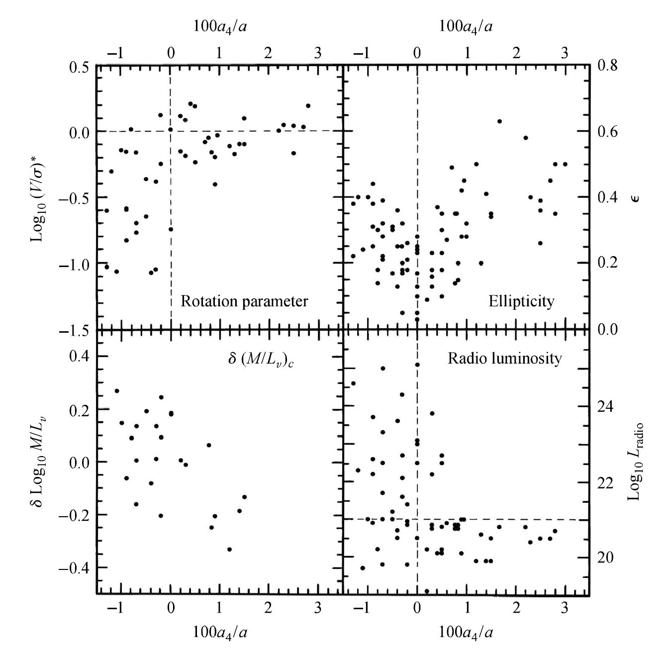
Fig. 4.24 The correlations of various parameters with \(a_4\) (isophotal shape). “Disky” ellipticals have a positive \(a_4\), while “boxy” ellipticals have a negative \(a_4\). Image Credit: Carroll & Ostlie (2007). Figure adapted from Kormendy & Djorgovski (1989).#
Figure 4.24 shows the correlations of various quantities with the isophotal Fourier parameter \(a_4\) (measured in units of \(100a_4/a_o\)).
The upper left-hand panel illustrates that disky galaxies tend to rotationally supported (with larger values of \(\left(v/\sigma\right)^*\)), while boxy galaxies are largely pressure-supported.
The lower left-hand panel indicates the deviation of the core mass-to-light ratio (measured in the \(V\) band) from the average value for galaxies of the same luminosity; boxy galaxies tend to have higher-than-average ratios, while disky galaxies have lower-than-average values.
The lower right-hand panel shows that boxy ellipticals tend to be much brighter at radio wavelengths that are disky galaxies. The spread in radio luminosities of boxy galaxies is quite large, while the variation in radio luminosity is much smaller.
The upper right-hand panel indicates that ellipticity (and therefore Hubble type) tends to increase with the absolute value of \(a_4\). This suggests that two galaxies of identical Hubble type could have very different characteristics when other physical parameters are considered.
For instance, two E4 galaxies (\(\epsilon = 4\)) could have one be rotationally supported (\(a_4 >0\)) while the other is pressure-supported \(a_4 <0\). The former would probably have a core mass-to-light ratio lower than average, while the latter galaxy would have a higher-than-average core mass-to-light ratio. The former galaxy would have a low radio luminosity and the latter might have a much higher radio luminosity.
Other parameters seem to associated with the boxiness or diskiness of a galaxy.
Rotationally supported disky galaxies have relatively large ratios of rotational angular momentum to mass (i.e., specific angular momentum), where pressure-supported boxy galaxies have rather low ratios.
Boxy galaxies are frequently observed to contain counter-rotating cores, while disky galaxies rarely posses counter-rotating cores.
Disky galaxies generally have rotational symmetries that are oblate, and boxy galaxies tend to be much more triaxial.
It is likely that the degree of boxiness among galaxies represents a continuum rather than two distinctly different classes of objects. Apparently some \(90\%\) of all ellipticals are generally disky in nature. Disky galaxies may simply represent an extension of the sequence of S0-type galaxies to progressively smaller disk-to-bulge ratios, and some disky galaxies are actually misclassified S0 galaxies. Boxy galaxies may represent a tell-tale signature of some level of environmental evolution (e.g., tidal interactions or mergers).
4.4.8. The Relative Numbers of Galaxies of Various Hubble Types#
The relative numbers of galaxies of various Hubble types is usually represented by the luminosity function \(\phi(M)\ dM\). This defines the number of galaxies in a particular sample that have absolute magnitudes between \(M\) and \(M+dM\).
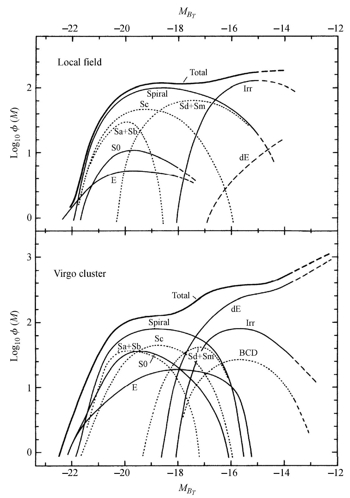
Fig. 4.25 Luminosity functions for two sample galaxies: near the Milky Way (top panel) and located near the Virgo cluster (bottom panel). The zero point of the \(\log_{10} \phi(M)\) axis is arbitrary. Image Credit: Carroll & Ostlie (2007). Figure adapted from Binggeli, Sandage, & Tammann (1988).#
Figure 4.25 shows the luminosity function for two samples: in the vicinity of the Milky Way and for a sample of galaxies in the Virgo cluster. The total luminosity function in either environment is the sum of the individual luminosity functions of each Hubble type.
In an attempt to find a general analytic fit to galactic luminosity functions, Paul Schechter proposed the functional form
In both forms, \(\alpha\) and \(L^*\) (or \(M^*\)) are free parameters that are used to obtain the best possible fit to the available data. For the data in Fig. 4.25,
\(\alpha = -1\) and \(M_B^* = -21\) for the local field of galaxies near the Milky Way,
\(\alpha = -1.24 \pm 0.02\) and \(M_B^* = -21 \pm 0.7\) for the Virgo cluster.
Although the values are similar, it is clear that there is not a universal luminosity function. Instead each luminosity function depends on the environment of the particular sample of galaxies.
In either environment of Fig. 4.25, the dE and dwarf irregular galaxies represent the largest fraction of all galaxies, even though S- and E-type galaxies are the most prominent in terms of both cluster luminosity and mass.
Although spirals represent the largest fraction of bright galaxies in each case, there is a somewhat higher proportion of ellipticals in the Virgo cluster. When the Virgo cluster is compared with the much larger and more densely populated Coma cluster the relative numbers of spirals and ellipticals change dramatically.
In the Virgo cluster: \(12\%\) E, \(26\%\) S0, and \(62\%\) S+Ir
In the Coma cluster: \(44\%\) E, \(49\%\) S0, and only \(7\%\) S+Ir
This is evidence that environment plays a role in galaxy formation and/or evolution.
4.5. Homework#
Problem 1
The absolute magnitude of M101 (an Sc galaxy) is \(M_B = -21.51\).
(a) Estimate its isophotal radius \((R_{25}\)) at \(25\ B-\text{mag/arcsec}^2\).
(b) Use the Tully-Fisher relation to estimate the rotational velocity of M101.
(c) Estimate the angular rotation speed of a star at \(R_{25}\) in units of \(arcsec/yr\).
Problem 2
Beginning with the general expression for the position vector in rectangular coordinates \(\mathbf{r} = x\hat{\mathbf{i}} + y\hat{\mathbf{j}} + z\hat{\mathbf{k}},\) show that the vector can be represented in cylindrical coordinates as \(\mathbf{r} = R\hat{\mathbf{e}}_R + z\hat{\mathbf{e}}_z\).
Problem 3
NGC 2639 is an Sa galaxy with a measured maximum rotational velocity of \(324\ \rm km/s\) and an apparent magnitude of \(B = 12.22\) (after making corrections for extinction).
(a) Estimate its absolute magnitude in the \(B\) band from the Tully-Fisher relation.
(b) Determine the distance to NGC 2639 using its distance modulus. See the Modern Astro notes.
(c) What is the galaxy’s radius \((R_{25})\) at a surface brightness of \(25\ B-\text{mag/arcsec}^2\)?
(d) Find the mass of NGC 2639 that is interior to \(R_{25}\).