9. Cosmology#

9.1. Newtonian Cosmology#

On December 27, 1831, the Beagle sailed out of Plymouth, England and was crowded with $74$ people, one of whom was Charles Darwin. During stops in South America, the Galapagos Islands, Tahiti, New Zealand, and Australia, he exercised his formidable powers of observation. In 1859, Darwin published On the Origin of Species, which marked the first time people began to comprehend their own origins from a naturalistic perspective.

Other discoveries followed during the next 100 years, with careful observations and brilliant deductions uncovering more about our beginnings. The discovery of DNA and plate tectonics revealed the mechanism by which we and our planet evolved. The ideas of stellar nucleosynthesis explained the manufacture of the chemical elements by stars, implying the origin of our corporeal bodies and the ground on which we walk. Even the universe itself was found to be expanding. In 1964, two researchers at Bell Laboratories measured the afterglow of the Big Bang, which provided compelling evidence for the explosive origin of everything in existence.

Cosmology is the study of the origin and evolution of the universe. However, there isn’t a single perspective for us to consider. Some insights can be gained by discussing the expansion of the universe through Newtonian mechanics, the discovery and implications of the cosmic microwave background radiation, the introduction of a geometrical universe through general relativity, and some key parameters that may be measured observationally.

9.1.1. Olber’s Paradox#

Newton believed in an infinite static universe filled with a uniform scattering of stars. If the distribution of matter did not extend forever, then it would collapse inward due to its own self-gravity. However, Edmund Halley worried about a sky filled with an infinite number of stars. Why then, is the sky dark at night?

This question was posed most strongly by Heinrich Olbers. Olbers argued (in 1823) that

if we live in an infinite, transparent universe filled with stars,
then in any direction one looks in the night sky, one’s line of sight will fall on the surface of a star.

This conclusion is valid regardless of whether the stars are uniformly distributed or grouped in galaxies. Olbers’ argument was so strong that its disagreement with the obvious fact that the night sky was indeed dark became known as Olbers’ paradox.

Olbers believed that the answer to this paradox was that space is not transparent. The ideas of thermodynamics were still being developed at that time, and Olbers could not appreciate that is answer was incorrect. The flaw was that any obscuring matter hiding the stars beyond would be heated up by the starlight until it glowed as brightly as a stellar surface.

Surprisingly, the first essentially correct answer came from Edgar Allan Poe (see this history). Poe proposed that because light has a finite speed and the universe is not infinitely old, then the light from the most distant sources has not yet arrived. This solution was independently put on a firm scientific foundation by Lord Kelvin (William Thomson). In more modern terms, the solution to Olbers’ paradox is that our universe is simply too young for it to be filled with light.

Note

It is sometimes argued that the cosmological redshift caused by the expansion of the universe is responsible for the darkness of the night sky because it shifts starlight out of the visible spectrum. In fact, this effect is much too small to contribute significantly to a dark night sky.

9.1.2. The Cosmological Principle#

Hubble’s law appears as a natural outcome of an expanding universe that is both isotropic and homogenous (i.e., appearing the same in all directions and at all locations). This crucial assumption of an isotropic and homogenous universe is called the cosmological principle.

To show that the expansion of the universe appears the same to all observers at all locations, consider a triangle with the Earth at the origin of the coordinate system and two galaxies ($A$ and $B$) located at the other two vertices. The galaxies can be located along two sides of the triangle using the position vectors $\mathbf{r}_A$ and $\mathbf{r}_B$ for galaxy $A$ and $B$, respectively. The other side of the triangle can then be defined by the difference vector $\mathbf{r}_B - \mathbf{r}_A$.

According to Hubble’s law, the recessional velocities of the two galaxies are described using the respective position vectors as

\[\begin{align*} \mathbf{v}_A &= H_o \mathbf{r}_A, \\ \mathbf{v}_B &= H_o \mathbf{r}_B. \end{align*}\]

The recessional velocity of galaxy $B$ as seen by an observer in galaxy $A$ is therefore

\[\begin{align*} \mathbf{v}_B - \mathbf{v}_A &= H_o\mathbf{r}_B - H_o\mathbf{r}_A, \\ &= H_o\left(\mathbf{r}_B - \mathbf{r}_A, \right), \end{align*}\]

so the observer in galaxy $A$ sees all of the other galaxies in the universe moving away with recessional velocities described by the same Hubble’s law as on Earth.

Although the value of the Hubble “constant” $H_o$ is assumed to be equivalent for all observers, it is actually a function of time $H(t)$. If the present time is $t_o$, then $H_o \equiv H(t_o).$

9.1.3. A Simple Pressureless “Dust” Model of the Universe#

To develop an understanding of how the expansion of the universe varies with time, imagine a universe with a pressureless “dust” of uniform density $\rho(t)$ and choose an arbitrary point for the origin. Unlike the actual universe, this model universe is both perfectly isotropic and homogenous at all scales. The pressureless dust represents all of the matter in the universe after being homogenized and uniformly dispersed.

Note

It should not be confused with the physical dust grains found throughout the ISM. There are no photons or neutrinos in this single-component model of the universe.

As the universe expands, the dust is carried radially outward from the origin. Let $r(t)$ be the radius of a thin spherical shell of mass $m$ at time $t$. This shell of mass expands along with the universe with a recessional velocity $v(t) =dr(t)/dt$, so it always contains the same dust particles. Then the mechanical energy $E$ of the shell is

\[ K(t) + U(t) = E.\]

As the shell expands, the gravitational pull from the mass inside causes the kinetic energy $K$ to decrease while the gravitational potential energy $U$ increases. Note that the mass outside the shell does not contribute to the gravitational force on the shell.

By conservation of energy, the total energy $E$ of the shell does not change as the shell moves outward. The total energy of the shell can be written in terms of two constants $k$ and $\varpi$, such that $E = -\frac{1}{2}mc^2 k\varpi^2$. The constant $k$ has units of $1/\text{length}^2$, where the other constant $\varpi$ labels the present radius of the shell (i.e., $r(t_o) = \varpi$). The conservation of the mass shell’s energy is then

(9.1)#\[\frac{1}{2}mv^2(t) - \frac{GM_rm}{r(t)} = -\frac{1}{2}mc^2 k\varpi^2,\]

where $M_r$ describes the mass interior to the shell, or $M_r = \frac{4}{3}\pi r^3(t) \rho(t).$

Although the radius of the shell and the density of the dust are continually changing, the combination $r^3(t)\rho(t)$ does not vary because the mass interior to a specific shell remains constant as the universe as the universe expands. Simplifying Eq. (9.1) by canceling the $m$ and substituting for $M_r$ gives

(9.2)#\[v^2 - \frac{8}{3}\pi G\rho r^2 = -c^2 k\varpi^2.\]

The constant $k$ determines the ultimate fate of this universe:

If $k>0$, the total energy of the shell is negative, and the universe is bounded, or closed. The expansion will someday halt and reverse itself.
if $k<0$, the total energy of the shell is positive, and the universe is unbounded, or open. The expansion will continue forever.
If $k=0$, the total energy fo the shell is zero, and the universe is flat (neither open nor closed). The expansion will continue to slow down, coming to a halt only as $t\rightarrow \infty$ and the universe is infinitely dispersed.

The terms closed, open, and flat should be understood as describing the dynamics of the universal expansion, however these terms will be reinterpreted later to describe the geometry of spacetime.

The cosmological principle requires that the expansion proceed in the same way for all shells. The time required for every shell to double its distance from the origin is assumed to be the sam. This means that the radius of a particular shell at any time can be written as

(9.3)#\[\begin{align} r(t) = R(t)\varpi, \end{align}\]

which defines the coordinate distance $r(t)$. The comoving coordinate $\varpi$ labels a shell and follows it as it expands. The dimensionless scale factor $R(t)$ is the same for all the shells and describes the expansion (i.e., cosmological redshift). Note that $R(t_o) = 1$ corresponds to $r(t_o) = \varpi$. The scale factor $R$ is equal to $R_{\rm emit}/R_{\rm obs}$. Thus $R$ and the redshift $z$ are related by

(9.4)#\[\begin{align} R = \frac{1}{z + 1}. \end{align}\]

The statement that $r^3\rho$ does not vary for a specific shell means that $R^3\rho$ also remains constant for all shells (since $R(t_o)=1$),

(9.5)#\[\begin{align} R^3(t)\rho(t) = R^3(t_o) \rho(t_o) = \rho_o, \end{align}\]

where $\rho_o$ is the density of the dust-filled universe at the present time. Relating this to the redshift, we find that

(9.6)#\[\begin{split}\rho(t) &= \frac{\rho_o}{R^3(t)}, \\ \rho(z) &= \rho_o \left(1 + z \right)^3,\end{split}\]

which gives the average density fo the universe as observed at redshift $z$. The above equations are valid only for a universe consisting of pressureless dust.

9.1.4. The Evolution of the Pressureless “Dust” Universe#

The evolution of our Newtonian universe begins with the Hubble parameter $H(t)$ written in terms of the scale factor. The Hubble law is

(9.7)#\[v(t) = H(t)r(t) = H(t)R(t)\varpi.\]

The left-hand side can be written through the time derivative of $r(t)$ as

(9.8)#\[\begin{align} v(t) = \frac{dR(t)}{dt}\varpi. \end{align}\]

Substituting into the above equation and solving for $H(t)$ to get

(9.9)#\[\begin{align} \frac{dR(t)}{dt}\varpi &= H(t)R(t)\varpi, \\ H(t) &= \frac{1}{R(t)}\frac{dR(t)}{dt}. \end{align}\]

Substituting using the Eq. (9.7) in Eq. (9.2) and then the above relation for $H(t)$ gives

(9.10)#\[\left(H^2 - \frac{8}{3}\pi G\rho \right) R^2 = -kc^2,\]

(9.11)#\[\begin{align} \left[\left(\frac{1}{R}\frac{dR}{dt}\right)^2 - \frac{8}{3}\pi G\rho \right] R^2 &= -kc^2. \end{align}\]

The left-hand sides apply to all shells and involve the functions $H(t)$, $\rho(t)$, and $R(t)$, while the right-hand sides are constant (the same for all positions and times). Using $\rho = \rho_o/R^3$, the relation becomes

(9.12)#\[\left( \frac{dR}{dt}\right)^2 - \frac{8\pi G\rho_o}{3R} = -kc^2.\]

This result will be used to describe the expansion of the universe.

The motion of the mass shells in the three universes (open, flat, or closed) can now be considered. Starting with the flat universe $(k=0)$, corresponding to each shell expanding at exactly its escape velocity. The critical density $\rho_c(t)$ represents the homogeneous solution $(k=0)$ to Eq. (9.10) as

(9.13)#\[\begin{align} \rho_c(t) = \frac{3H^2(t)}{8\pi G}. \end{align}\]

To evaluate this at the present time, it is useful to know the Hubble constant in conventional units as

(9.14)#\[\begin{align} H_o &=& 100/h\ {\rm km/s/Mpc} &=& 3.24/h \times 10^{-18}\ {\rm s^{-1}}, \\ [H_o]_{\rm WMAP} &=& 71\ {\rm km/s/Mpc} &=& 2.30 \times 10^{-18}\ {\rm s^{-1}}. \end{align}\]

Then, the present value of the critical density is

(9.15)#\[\begin{align} \rho_{c,o} &= \frac{3H_o^2}{8\pi G}, \\ &= 1.88/h^2 \times 10^{-26}\ {\rm kg/m^3}, \\ &= 9.47 \times 10^{-27}\ {\rm kg/m^3}. \end{align}\]

This is equivalent to about 6 $\rm H$ atoms per cubic meter. The WMAP value of the average density of baryonic matter in the universe is about $4\%$ of the critical density,

(9.16)#\[\begin{align} \rho_{\rm b,o} = 4.17 \times 10^{-28}\ {\rm kg/m^3}, \qquad \text{for h = 0.71}\end{align}\]

or $1\ \rm H$ atom per $4\ \rm m^3$ of space. Baryonic matter refers to normal matter composed of protons and neutrons. This value is consistent with that obtained from comparing the theoretical and observed abundance of light elements (e.g., ${^3}\rm He$ and ${^7}\rm Li$) that were formed in the early universe. The density of nonbaryonic dark matter is not included in the value of $\rho_{\rm b,o}$.

Our model universe of pressureless dust includes both types of matter: luminous and dark. The ratio of a measured density to the critical density is an important and is defined as the density parameter,

(9.17)#\[\begin{split}\Omega(t) &\equiv \frac{\rho(t)}{\rho_{\rm c}(t)}, \\ &= \frac{8\pi G\rho(t)}{3H^2(t)}, \\ \Omega_o &= \frac{8\pi G\rho_o}{3H_o^2}.\end{split}\]

Table 9.1 Mass-to-light ratios and density parameters (adapted from Binney & Tremaine (1987) and Schramm (1991))#
Method	$M/L$ ($M_\odot/L_\odot$)	$\Omega_o$
Solar neighborhood	$3$	$0.002 h^{-1}$
Elliptical galaxy cores	$12 h$	$0.007$
Local escape speed	$30$	$0.018 h^{-1}$
Satellite galaxies	$30$	$0.018 h^{-1}$
Magellanic Stream	$>80$	$>0.05 h^{-1}$
X-ray halo of M87	$>750$	$>0.46 h^{-1}$
Local Group timing	$100$	$0.06 h^{-1}$
Galaxy groups	$260 h$	$0.16$
Galaxy clusters	$400 h$	$0.25$
Gravitational lenses	$--$	$0.1-0.3$
Big Bang nucleosynthesis	$--$	$0.065 \pm 0.045$

Table 9.1 shows the mass-to-light ratios of a variety of astronomical systems, along with the density parameters. Almost all of the values were obtained by studying gravitational effects (including both baryonic and dark matter), where the Big Bang nucleosynthesis is the exception. There is a significant trend that more extensive systems have larger mass-to-light ratios and density parameters, but the density parameters seem to saturate at a maximum value of $\Omega_o \simeq 0.3$. This is consistent with the WMAP result (using $h = 0.7) for the average density of all types of matter:

(9.18)#\[\begin{align} [\Omega_{\rm m,o}]_{\rm WMAP} &= \frac{0.135^{+0.008}_{-0.009}}{h^2}, \\ &= 0.27 \pm 0.04, \end{align}\]

and a mass density of

(9.19)#\[\begin{align} \rho_{\rm m,o} &= 2.56 \times 10^{-27}\ {\rm kg/m^3}. \end{align}\]

The WMAP value of the density parameter for only baryonic matter:

(9.20)#\[\begin{align} \left[ \Omega_{\rm b,o}\right]_{\rm WMAP} &= \frac{0.0224 \pm 0.0009}{h^2}, \\ &= 0.044 \pm 0.004. \end{align}\]

According to the WMAP results baryonic matter accounts for only about $0.044/0.027 = 16\%$ of the matter in the universe, while nonbaryonic dark matter accounts for the remaining $84\%$.

The general characteristics of the expansion of the pressureless dust filled universe can be determined. From the relationship between density and redshift (Eq. (9.6)), along with the density parameter (Eq. (9.17)), we have

(9.21)#\[\begin{split}\frac{\Omega}{\Omega_o} &= \frac{\rho}{\rho_o}\frac{H_o^2}{H^2} = (1+z)^3 \frac{H_o^2}{H^2}, \\ \Omega H^2 &= (1+z)^3 \Omega_o H_o^2.\end{split}\]

Another relation between $\Omega$ and $H$ comes from combining the density parameter (Eq. (9.17)) with the energy from Hubble’s law (Eq. (9.10)) to get

(9.22)#\[\begin{split}H^2\left(1-\Omega \right)R^2 &= -kc^2, \\ H_o^2\left(1-\Omega_o \right) &= -kc^2. \qquad (t=t_o)\end{split}\]

This confirms that

If $\Omega_o > 1$, then $k>0$ and the universe is closed.
If $\Omega_o < 1$, then $k<0$ and the universe is open.
If $\Omega_o = 1$, then $k=0$ and the universe is flat.

This model deals with a one-component universe of pressureless dust, where a more realistic multicomponent model will show that the mass density parameter alone is not enough for us to draw any conclusions about the fate of our physical universe.

Substituting $R^2 = 1/(1+z)^2$ and equating the two relations in Eq. (9.22) produces

(9.23)#\[\begin{align} H^2(1-\Omega)R^2 &= H_o^2(1-\Omega_o), \\ H^2(1-\Omega) &= H_o^2(1-\Omega_o)(1+z)^2. \end{align}\]

Thus we have two equations (Eqs. (9.22) and (9.21)), with two unknowns ($\Omega$ and $H$), which can be solved to find

(9.24)#\[H = H_o(1+z)\sqrt{1+\Omega_o z}\]

and

(9.25)#\[\begin{split}\Omega &= \frac{\Omega_o z+\Omega_o }{1+\Omega_o z}, \\ &= \frac{(1 + \Omega_o z)+\Omega_o - 1 }{1+\Omega_o z}, \\ & = 1 + \frac{\Omega_o - 1 }{1+\Omega_o z}.\end{split}\]

Equation (9.24) implies that at very early times ($R\rightarrow 0$ and $z\rightarrow \infty$), the Hubble parameter diverges ($H \rightarrow \infty$).

Equation (9.25) shows that the sign of $(\Omega -1)$ does not change, and that if $\Omega = 1$, then $\Omega = 1$ at all times.

The character of the universe does not change as the universe evolves; it is either always closed, open, or flat.
At very early times (as $z\rightarrow \infty$), the density parameter $\Omega \rightarrow 1$ regardless of the present value of $\Omega_o$. The early universe was essentially flat.

The assumption of a flat early universe will greatly simplify the description of the first few minutes of the universe.

Exercise 9.1

When the universe was ${\sim}3$ minutes old, protons and neutrons combined to form helium nuclei. This occurred at a redshift of $z = 3.68 \times 10^8$.

Using the WMAP value of $\Omega_{\rm m,o} = 0.27$ for $\Omega_o$, find the density parameter $\Omega$ at the time of helium formation.

Equation (9.25) directly depends on the initial density parameter $\Omega_o$ and the redshift $z$ to produce $\Omega$. Thus, we can directly substitute the given values into the equation by

(9.26)#\[\begin{align} \Omega = 1 + \frac{0.27 - 1}{1+ (0.27)(3.68\times 10^8)} = 0.99999999265. \end{align}\]

At even earlier times the value of $\Omega$ is much closer to $1$ and thus contains a much longer string of nines.

Omega_o = 0.27
z = 3.68e8

Omega = 1 + (Omega_o - 1)/(1 + Omega_o*z)
print("The value for Omega is %1.11f." % Omega)

The value for Omega is 0.99999999265.

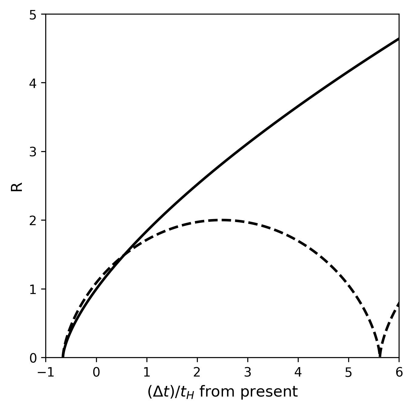
The expansion of a flat, one-component universe of pressureless dust as a function of time comes form solving Eq. (9.12) with $k=0$ ($\rho_o = \rho_{c,o}$ and $\Omega_o = 1$), which produces

(9.27)#\[\begin{align} \left(\frac{dR}{dt} \right)^2 = \frac{8\pi G \rho_{c,o}}{3R}. \end{align}\]

Taking the square root of each side and integrating (with $R(t=0) = 0$) gives

(9.28)#\[\begin{align} \int_0^R \sqrt{R^\prime}dR^\prime &= \sqrt{\frac{8}{3}\pi G \rho_{c,o}} \int_0^t dt^\prime, \\ \frac{2}{3}(R^\prime)^{3/2} \biggr \vert_0^R & = \sqrt{\frac{8}{3}\pi G \rho_{c,o}} t^\prime \biggr \vert_0^t, \\ \frac{2}{3}R^{3/2} &= \sqrt{\frac{8}{3}\pi G \rho_{c,o}} t. \end{align}\]

Now, we can solve for the scale factor of a flat universe $R_{\rm flat}$ as

(9.29)#\[\begin{align} R_{\rm flat} &= \left[\left(\frac{9}{4}\right) \left(\frac{8}{3}\right) \pi G \rho_{c,0}\right]^{1/3} t^{2/3}, \\ &= \left(6\pi G \rho_{c,0}\right)^{1/3} t^{2/3}. \end{align}\]

We can rewrite the critical density in terms of the Hubble time as

(9.30)#\[\begin{align} \rho_{c,o} = \frac{3}{8\pi G} H_o^2 = \frac{3}{8\pi G} \frac{1}{t_H^2} \end{align}\]

and substituting back into the equation for $R_{\rm flat}$ produces

(9.31)#\[\begin{align} R_{\rm flat} = \left[ \frac{3}{2} \left(\frac{t}{t_H}\right) \right]^{2/3}. \end{align}\]

If $\Omega_o \neq 1$, the density is not equal to the critical density and Eq. (9.12) is harder to solve. If $\Omega_o > 1$, the universe is closed and the solution can be parametrized as

(9.32)#\[\begin{align} R_{\rm closed} &= \frac{4\pi G \rho_o}{3kc^2} \left[1-\cos(x) \right], \\ &= \frac{1}{2} \frac{\Omega_o}{\Omega_o - 1} \left[1-\cos(x) \right], \end{align}\]

and

(9.33)#\[\begin{align} t_{\rm closed} &= \frac{4\pi G \rho_o}{3k^{3/2}c^3} \left[x-\sin(x) \right], \\ &= \frac{1}{2 H_o} \frac{\Omega_o}{\left(\Omega_o - 1\right)^{3/2}} \left[x-\sin(x) \right], \end{align}\]

where the variable $x \geq 0$ parametrizes the solution.

import matplotlib.pyplot as plt 
import numpy as np 

def scale_factor(Omega_o,x):
    if Omega_o == 1:
        return (1.5*x)**(2./3.)
    elif Omega_o > 1:
        t_cl = 0.5*Omega_o/(Omega_o-1)**1.5*(x-np.sin(x))
        R_cl = 0.5*Omega_o/(Omega_o-1)*(1-np.cos(x))
        return t_cl,R_cl
    elif Omega_o < 1:
        t_op = 0.5*Omega_o/(Omega_o-1)**1.5*(np.sinh(x)-x)
        R_op = 0.5*Omega_o/(Omega_o-1)*(np.cosh(x)-1)
        return t_op, R_op

fs = 'large'

fig = plt.figure(figsize=(5,5),dpi=300)
ax = fig.add_subplot(111)

x = np.arange(-0.66,9,0.01)
ax.plot(x,scale_factor(1,x+0.66),'k-',lw=2)

x = np.arange(0,9,0.01)
t, R = scale_factor(2,x)
ax.plot(t-0.66,R,'k--',lw=2)

#t, R = scale_factor(0.5,x)
#ax.plot(t-0.66,R,'r--',lw=2)

ax.set_ylim(0,5)
ax.set_xlim(-1,6)
ax.set_ylabel("R",fontsize=fs)
ax.set_xlabel("$(\Delta t)/t_H$ from present", fontsize=fs);

9.1.5. The Age of the Pressureless “Dust” Universe#

9.1.6. The Lookback Time#

9.1.7. Extending Our Simple Model to Include Pressure#

9.1.8. The Deceleration Parameter#

9.2. The Cosmic Microwave Background (CMB)#

9.2.1. The Steady-State Model of the Universe#

9.2.2. The Cooling of the Universe after the Big Bang#

9.2.3. The Discovery of the CMB#

9.2.4. The Dipole Anisotropy of the CMB#

9.2.5. The Sunyaev-Zel’dovich Effect#

9.2.6. Does the CMB Constitute a Preferred Frame of Reference?#

9.2.7. A Two-component Model of the Universe#

9.2.8. Neutrino Decoupling#

9.2.9. The Energy Density of Relativistic Particles#

9.2.10. Transition from the Radiation to the Matter Era#

9.2.11. Expansion in the Two-component Model#

9.2.12. Big Bang Nucleosynthesis#

9.2.13. The origin of the CMB#

9.2.14. The Surface of Last Scattering#

9.2.15. The Conditions at Recombination#

9.2.16. The Dawn of Precision Cosmology#

9.3. Relativistic Cosmology#

9.3.1. Euclidean, Elliptic, and Hyperbolic Geometries#

9.3.2. The Robertson-Walker Metric for Curved Spacetime#

9.3.3. The Friedmann Equation#

9.3.4. The Cosmological Constant#

9.3.5. The Effects of Dark Energy#

9.3.6. The $\Lambda$ Era#

9.3.7. Model Universes on the $\Omega_{m,0}-\Omega_{\Lambda,0}$ Plane#

9.4. Observational Cosmology#

9.4.1. The Origin of the Cosmological Redshift#

9.4.2. Distances to the Most Remote Objects in the Universe#

9.4.3. The Particle Horizon and the Horizon Distance#

9.4.4. The Arrival of Photons#

9.4.5. The Maximum Visible Age of a Source#

9.4.6. The Comoving Coordinate $\varpi(z)$#

9.4.7. The Proper Distance#

9.4.8. The Luminosity Distance#

9.4.9. The Redshift Magnitude Relation#

9.4.10. Angular Diameter Distance#

9.5. Homework#

Problem 1

Show by substitution that the following equations are solutions to Eq. (9.12) for a closed universe $(k>0)$:

(9.34)#\[\begin{align} R_{\rm closed} &= \frac{4\pi G\rho_o}{3kc^2}\left[1-\cos(x)\right],\\ t_{\rm closed} &= \frac{4\pi G\rho_o}{3k^{3/2}c^3}\left[x-\sin(x)\right]. \end{align}\]

Problem 2

Show by substitution that the following equations are solutions to Eq. (9.12) for an open universe $(k<0)$:

(9.35)#\[\begin{align} R_{\rm open} &= \frac{4\pi G\rho_o}{3|k|c^2}\left[\cosh(x) - 1\right],\\ t_{\rm open} &= \frac{4\pi G\rho_o}{3|k|^{3/2}c^3}\left[\sinh(x)-x\right]. \end{align}\]

Method	\(M/L\) (\(M_\odot/L_\odot\))	\(\Omega_o\)
Solar neighborhood	\(3\)	\(0.002 h^{-1}\)
Elliptical galaxy cores	\(12 h\)	\(0.007\)
Local escape speed	\(30\)	\(0.018 h^{-1}\)
Satellite galaxies	\(30\)	\(0.018 h^{-1}\)
Magellanic Stream	\(>80\)	\(>0.05 h^{-1}\)
X-ray halo of M87	\(>750\)	\(>0.46 h^{-1}\)
Local Group timing	\(100\)	\(0.06 h^{-1}\)
Galaxy groups	\(260 h\)	\(0.16\)
Galaxy clusters	\(400 h\)	\(0.25\)
Gravitational lenses	\(--\)	\(0.1-0.3\)
Big Bang nucleosynthesis	\(--\)	\(0.065 \pm 0.045\)