Gaia & Oxygen
Contents
8. Gaia & Oxygen#
8.1. Gaia: An Integrated System#
In 1973, James Lovelock and Lynn Margulis introduced a hypothesis about the conditions for which life might need to continue on a habitable world. It is insufficient to focus on the origins of life, but there are other processes that could be necessary for the propagation of life over billions of years. The known biogeochemical cycles (for carbon and nitrogen) introduce feedbacks between the organic biosphere and the inorganic geochemical environment. Early studies in atmospheric science showed that the principal gases \(\rm N_2\) and \(\rm O_2\) are cycled by the biosphere with a geometric mean residence time on the order of a few thousands of years. The paper by Lovelock & Margulis (1973) presents a view of the atmosphere as an extension of the biosphere rather just a product of geologic outgassing. Due to the feedbacks that regulate the internal geology, biology, and atmosphere of the Earth, the biosphere itself acts as an active adaptive control system to maintain the Earth in homeostasis called the Gaia hypothesis.
8.1.1. Theoretical Basis#
The discovery of a new organism and its habitat is sometimes instinctively framed as a purposeful structure that is crafted to suit the needs of the organism. For example, a bees nest provides a purpose that is distinctive from other non-social insects in that the ecosystem developed between the bees facilitates the construction of a monument to the hive. The organization of the tropical rainforest was not recognized a larger, complex system until the evidence of the cycling of essential elements was discovered. The emergence of a larger ecosystem (i.e., Gaia) may exist as a phenomenon that is necessary for living systems to thrive, and the lack of such an ecosystem might signify the differences in the observed biosphere in the Solar System.
One definition of life can be cast thermodynamically as the ability for a system to decrease the local entropy at the expense of the free energy taken from the environment (Bernal 1951). This may be expressed in the form of the continuity equation for entropy as
which depends on the internal creation rate of entropy \(\theta\), the density \(\rho\), and the entropy \(S\). The \(\nabla S\) signifies the outflow of entropy and the \(\rho(dS/dt)\) is the entropy’s rate of change within the enclosed region. From the Second Law of Thermodynamics, the creation rate of entropy \(\theta\) must be greater than or equal to zero, which prohibits both of the left-hand side terms from turning negative simultaneously. Note that this classification includes both vortices and flames, which may be too broad.
The thermodynamic definition of life serves to help the Gaia hypothesis by defining local changes of entropy as the product of a living entity that modifies the background environment through either physical or chemical disequilibrium. A human and a tree modify their respective environments in different ways in which is bears pointing out the pertinent thermodynamic processes.
A human takes in free energy in the form of the chemical potential contained in food and oxygen, while sustaining a low internal entropy through the excretion of waste chemicals and heat. The environment that receives the excess entropy includes the atmosphere and the transfer boundary includes the skin.
A tree takes in free energy directly from the Sun to sustain a high chemical potential gradient within the atmosphere on a planetary scale. The atmosphere receives the excess oxygen and the transfer boundary includes the tree’s leaves.
The boundaries between each of these organisms is arbitrary, where a more general boundary is between the atmosphere and interplanetary space. In this instance, the whole assembly of life contributes to the outgoing entropy flux from the Earth in the form of the long-wave IR radiation. The greenhouse effect is largely described abiotically and contributes to the expected entropy flux of a planet devoid of life. Therefore, the difference in entropy flux between a living and non-living planet could be a measure for identifying ‘Gaia’ (if such a thing exists).
8.1.2. Atmospheric Stability (Kirchner (2002))#
A key component of the Gaia hypothesis is feedbacks from biological systems that help regulate the environment which in turn facilitate their own survival. As a result, the biota co-evolves along with Earth’s environment throughout geologic time (Schneider & Londer (1984)). The consequences of feedbacks that emerge from the co-evolution can potentially be beneficial or detrimental to any given group of organisms. In the Gaia literature, a larger emphasis is placed on negative feedbacks that are beneficial to the organisms involved or the biota as a whole (Lenton (1998); Gillon (2000)).
Detecting life elsewhere in the galaxy depends on our observations of planetary atmospheres, which could uncover a host of evidence concerning potentially biological feedbacks. Although it may not be a sufficient condition, atmospheric stability does appear to be an enticing. Some of the relevant biological feedbacks include:
Negative feedbacks
Increased atmospheric \(\rm CO_2\) concentrations that stimulate increased photosynthesis and leads to carbon sequestration in biomass.
Warming that leads to drying (and thus sparser vegetation) and increased desertification in mid-latitudes, which can increase the planetary albedo and atmospheric dust concentrations.
Positive feedbacks
Warmer temperatures that increase soil respiration rates and release organic carbon stored in soils.
Warmer temperatures increase the frequency of wildfires, which leads to a net replacement of the older, larger trees with younger, smaller ones and results in a net release of carbon from forest biomass.
Higher atmospheric \(\rm CO_2\) concentrations may increase drought tolerance in plants and potentially lead to expansion of shrublands into deserts. This would reduce the planetary albedo and dust concentrations.
Warming that leads to the replacement of tundra by boreal (coniferous dominant) forest, which decreases the planetary albedo.
Warming of soils accelerates methane production over consumption, which leads to net methane release.
Warmer temperatures lead to the release of \(\rm CO_2\) and methane from high-latitude peatlands.
The above list of feedbacks in not exhaustive nor comprehensive, but it does show ways in which the biota can react to a changing atmosphere. The Gaia hypothesis proposes that some of these (maybe all) feedbacks lead to an emergent regulatory effect when taking multiple feedbacks into account. However, this remains to be seen and appears to contradict many scientists who believe that the positive feedbacks broadly outweigh the negative ones.
Our planet’s surface area is largely comprised (\({\sim}71\%\)) by water, where oceans hold \(96.5\%\) of all Earth’s water. Therefore, the interface between the oceanic biota and the atmosphere could be more important than the land-based effects. One outgrowth of the Gaia hypothesis suggests that oceanic phytoplankton might serve as a planetary thermostat by producing dimethyl sulfide, or \(\rm (CH_3)_2 S\), which is a precursor for cloud condensation nuclei and a response to a warming atmosphere (Charlson et al. (1987)).
However, paleoclimate data (Legrand et al. (1988); Kirchner (1990); Legrand et al. (1991)) indicate such a marine biological thermostat is hooked up backwards, where it exacerbates the cooling or warming trends (i.e., makes the planet colder when it is cold and warmer when it is warm). Moreover, dimethyl sulfide production in the Southern Ocean may be controlled by atmospheric dust, which supplies iron as a limiting nutrient. The Antarctic ice core record is consistent with this view, where a greater deposition of atmospheric dust occurs during glacial periods, along with high levels of dimethyl sulfide proxy compounds, lower concentrations of \(\rm CO_2\) and \(\rm CH_4\), and lower temperatures.
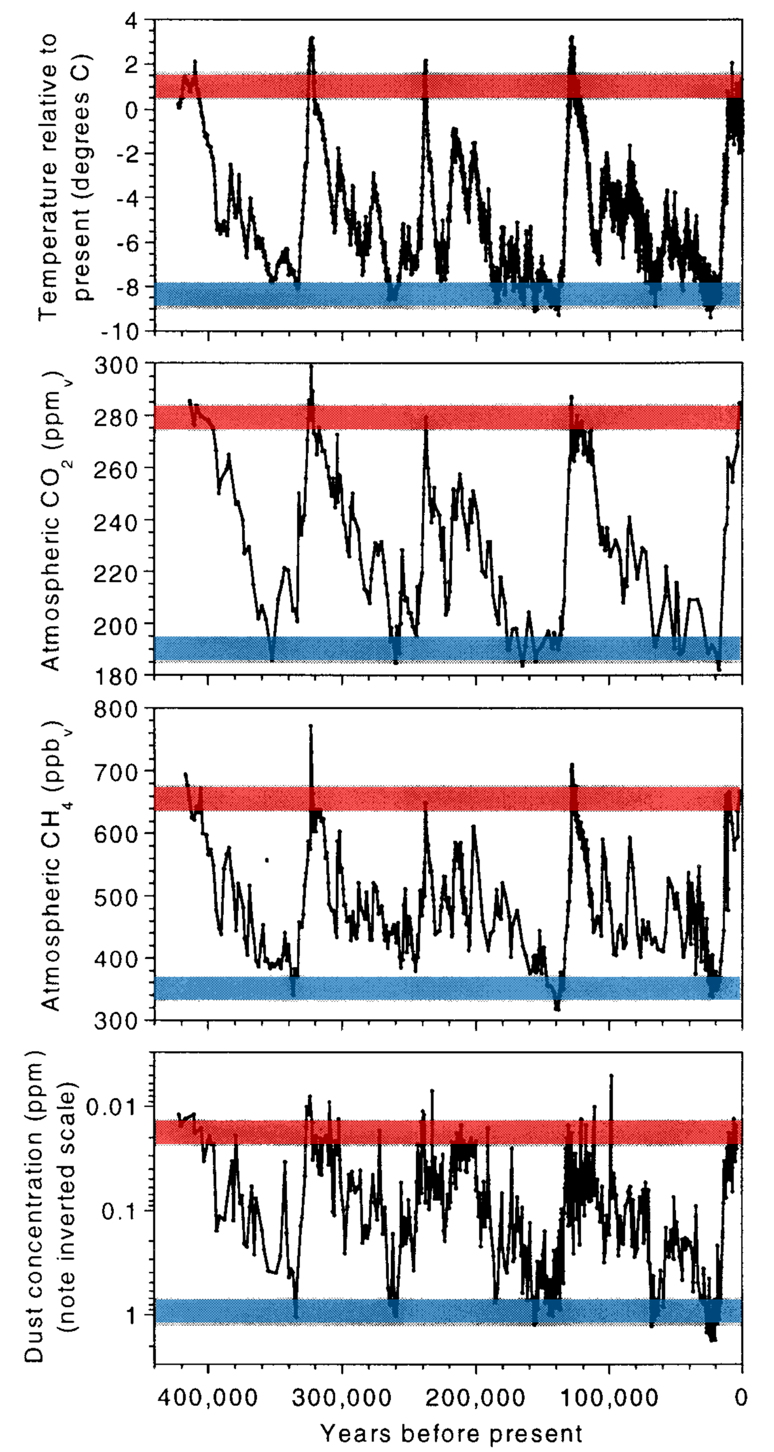
Fig. 8.1 The Vostok ice core record of atmospheric temperature, carbon dioxide \(\rm CO_2\), methane \(\rm CH_4\), and dust loading (data of Petit et al. (1999)). Glacial maxima (blue bands) and interglacials (red bands) exhibit relatively narrow ranges of concentrations and temperatures. The temperature, \(\rm CO_2\), and methane appear correlated, while the dust concentration (inverted scale) is anti-correlated (i.e., low dust allows for warmer temperatures). Figure credit: Kirchner (2002).#
8.1.3. Biologic Stability: DaisyWorld (Watson & Lovelock (1983))#
The Gaia hypothesis could be just wishful thinking, but there are some aspects that are testable (at least through computer simulation). One such scenario is through the parable of Daisyworld. Suppose there is a cloudless, Earth-like planet that consists of two types (black and white) of daisies on its surface. This is Daisyworld, where the color of the daisies and their extent can change some macroscopic properties of the planet’s atmosphere. Recall from the Chapter on Planetary Atmospheres that the basic energy balance model of the greenhouse effect depends on a planet’s reflectivity (or albedo), which in turn regulates the atmospheric temperature.
In Daisyworld, the combined area of the white daises will increase the planetary albedo, while the black daisies would decrease the albedo. We can model Daisyworld through coupled first-order differential equations that describe the changing combined area from the white \(A_w\) and black \(A_b\) daisies. Carter & Prince (1981) provided a mathematical framework that describes the epidemic spread of plants within an environment. The main parameters to include in the model are:
areas \(A_w\) and \(A_b\) covered by white and black daisies, respectively,
the area \(A_f\) of the fertile ground that is not yet covered by either species,
the normalized growth rate \(\beta\) (i.e., the percentage of daisies that appear per unit of time), and
the normalized death rate \(\gamma\) (i.e., the percentage of daisies that die per unit of time).
The area \(A_f\) of the fertile ground can be determined by defining the total area \(A\) available on the planetary surface. To make things easier, we can normalize the system so that we track the fractional area \(a\) of the daisies (i.e., \(a_w = A_w/A\); \(a_b = A_b/A\)) so that we can set the total area equal to unity. The fractional area of fertile ground \(a_f\) available at a given time is:
Watson and Lovelock (1983) prescribe a growth rate \(\beta\) for both types of daisies that is a parabolic function of the local temperature \(T_C\) in Celsius:
which is zero when the local temperature is \(5 \rm ^\circ C\) or \(40 \rm ^\circ C\). Note that the coefficient in front of the squared term is rounded and should be \(1/17.5^2\) to give a more exact representation. The growth rate is maximized when \(T_C = 22.5 \rm ^\circ C\). Putting all of this together, we can write the coupled differential equations as:
that describe how the fractional area of each type of daisies changes in response to the local temperature. The variation in area changes the overall albedo of the planet, which in turn affects the local temperature through the equation for the equilibrium temperature, or
which depends on the albedo of the planet \(\alpha\), Stefan-Boltzmann constant \(\sigma\), and surface flux \(\mathcal{F}\). The surface flux itself depends on the luminosity \(\mathcal{L}\) of the host star, the planet’s distance from the star \(d\), and is typically normalized relative to the Solar constant \(S\). The planetary albedo is determined by
The planetary albedo depends on the sum of the albedos including the white daises (\(\alpha_w = 0.75\)), black daisies (\(\alpha_b = 0.25\)) and the bare ground (\(\alpha_g = 0.5\)). The area of the bare ground \(a_g\) can be determined as the remaining ground that is not covered by black or white daisies (i.e., \(a_g = 1 - a_b - a_w\)). This linear superposition of albedos assumes that the planetary surface is flat instead of spherical, which also reduces the received flux by a factor of four. The incident energy is also redistributed across the surface, where Watson & Lovelock (1983) introduce a parameter \(q^\prime\) to modulate the effect on the effective temperature by the three different surfaces. This produces separate relations for the temperature due to the white \(T_w\) or black \(T_b\) daisies as:
The basic algorithm for Daisyworld can be implemented in python (see code below) or in your favorite language. The key is to divide the process into three functions, or methods, that calculate the
equilibrium temperature of the barren surface, white daisies, and black daisies;
change in area covered by the daisies over time; and
integrate the first-order differential equations and test for convergence.
The rest of the process depends on the initial parameters. In Watson & Lovelock (1983), they perform simulations that vary the luminosity of the host star while tracking the percent area coverage of daises and the effective temperature of the barren surface. Their initial conditions are given as:
Solar constant \(S_o = 1000\ \rm W/m^2\),
death rate \(\gamma = 0.3\)
albedo of bare ground \(\alpha = 0.5\),
albedo of black daises \(\alpha_b = 0.25\),
albedo of white daises \(\alpha_w = 0.75\),
redistribution factor \(q^\prime = 20\),
initial fractional area of white daisies \(a_w = 0.01\),
initial fractional area of black daisies \(a_b = 0.01\),
minimum fractional area of daisies \(a = 0.01\).
The final assumption is key to reproducing their results.
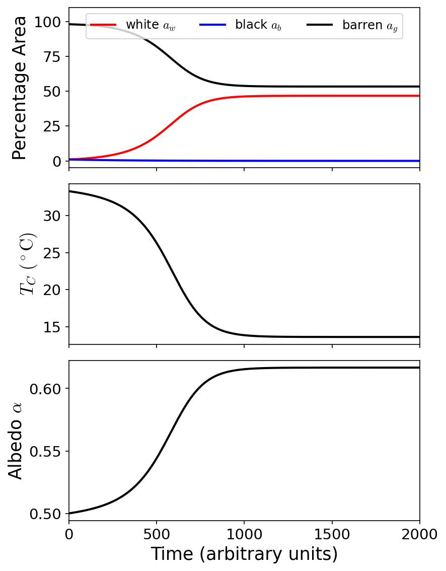
Fig. 8.2 Simulation of Daisyworld for 2000 time units to demonstrate the evolution for the percentage area of each surface (top), local temperature (middle), and albedo (bottom). This simulation assumes a Solar luminosity (\(1\ L_\odot\)) intersects a planet at \(1.167\ \rm AU\) to give a Solar constant \(S_o = 1000\ \rm W/m^2\). The white daisies dominate over the black daisies, which leads to a decrease in the local temperature due to the increased overall albedo.#
import numpy as np
import matplotlib.pyplot as plt
from scipy.constants import sigma
from matplotlib import rcParams
from myst_nb import glue

rcParams.update({'font.size': 14})
rcParams.update({'mathtext.fontset': 'cm'})

def T_eq(a_w,a_b):
    #Calculate the zeroth order equilibrium temperature from Stefan-Boltzmann Flux equation
    #a_w = fraction of surface area covered by white daisies at time t
    #a_b = fraction of surface area covered by black daisies at time t
    #sigma = Stefan-Boltzmann constant
    #qp = insolation factor from Watson & Lovelock(1983)
    F = L_star/semi**2*S_oplus
    a_g = 1 - (a_w + a_b) #fractional area of the ground not covered by daisies (i.e., bare ground)
    alpha = alpha_g*a_g + alpha_w*a_w + alpha_b*a_b #total albedo of the planet
    T_surf = ((1.-alpha)*F/sigma)**(1./4.)  #Equilibrium temperature in Kelvin
    T_w = qp*(alpha-alpha_w) + T_surf
    T_b = qp*(alpha-alpha_b) + T_surf
    return T_surf, T_w, T_b, alpha

def daisyworld(x,L,gamma):
    #x = [a_w,a_b]; state vector containing fractional areas
    #L = Luminosity of the host star in L_sun
    #gamma = death rate of daisies
    temp = np.zeros(len(x))
    a_g = 1. - (x[0] + x[1]) #fractional area of the ground not covered by daisies (i.e., bare ground)
    T_surf, T_w, T_b, alpha = T_eq(x[0],x[1]) # temperature of whole planet
    beta_w, beta_b = 0., 0.
    if T_w >= T_low and T_w <= T_hi and x[0]>=a_min:
        beta_w = 1. - beta_coeff*(T_ideal-T_w)**2 #growth rate of white daisies
    if T_b >= T_low and T_b <= T_hi and x[1]>=a_min:
        beta_b = 1. - beta_coeff*(T_ideal-T_b)**2  #growth rate of black daisies
    temp[0] = x[0]*(a_g*beta_w - gamma) #change in area occupied by white daisies
    temp[1] = x[1]*(a_g*beta_b - gamma) #change in area occupied by black daisies
    return temp

def euler(x,h,xtol,stop_integ):
    #integration by Euler's method
    #x = [a_w,a_b,T_surf]; state vector containing fractional areas and effective temperature
    #h = step size
    yp = x + h*daisyworld(x,L_star,gamma)
    T_surf, T_w, T_b, alpha = T_eq(yp[0],yp[1])
    yp[2] = T_surf
    yp[3] = alpha
    if np.abs(x[0]-yp[0])<xtol or np.abs(x[1]-yp[1])<xtol:
        stop_integ = True
    return yp, stop_integ

L_star = 1. #L = Luminosity of the host star in L_sun
S_oplus = 1000. #S_oplus = Flux Earth receives from the Sun; should be 1361 W/m^2
semi = 1. #semi = semimajor axis of the planet in AU
gamma = 0.3 #gamma = death rate of daisies
beta_coeff = 1./17.5**2
qp = 20. #insolation factor from Watson & Lovelock(1983)

#Temperature limits
T_low = 273.15 + 5 #lower limit for daisy growth
T_hi = 273.15 + 40 #upper limit for daisy growth
T_ideal = 273.15 + 22.5
a_min = 1e-2 #minimum area for daisies

#integration parameters
xtol = 1e-14
h = 0.01
max_iter = 1e5/h

#albedos
alpha_g = 0.5 # albedo of the ground not covered by daisies (i.e., bare ground)
alpha_w = 0.75 # albedo for the white daisies
alpha_b = 0.25 # albedo for the black daisies
fs = 'large'

#initial state
a_w, a_b = 1e-2, 1e-2 #initial areas covered by daisies
T_surf, T_w, T_b, alpha = T_eq(a_w,a_b) # temperature of whole planet
state = [[a_w,a_b,T_surf,alpha]]
#y, stop_integ = euler(state[-1],h,xtol,stop_integ)
#
#print(T_surf,T_w,T_b)
stop_integ = False
it = 0
while not stop_integ and it < max_iter: #stop integrating after convergence
    y, stop_integ = euler(state[-1],h,xtol,stop_integ)
    state.append([y[0],y[1],y[2],y[3]])
    it += 1
it = 2000
state = np.array(state)
fig = plt.figure(figsize=(6,9),dpi=150)
ax1 = fig.add_subplot(311)
ax2 = fig.add_subplot(312)
ax3 = fig.add_subplot(313)
iterations = range(0,len(state[:,0]))

ax1.plot(iterations,100*state[:,0],'r-',lw=2, label='white $a_w$')
ax1.plot(iterations,100*state[:,1],'b-',lw=2, label='black $a_b$ ')
ax1.plot(iterations,100*(1-state[:,0]-state[:,1]),'k-',lw=2, label='barren $a_g$')

ax1.legend(loc='upper center',fontsize='small',ncol=3)
ax1.set_ylabel("Percentage Area",fontsize=fs)
ax1.set_xticklabels([])
ax1.set_ylim(-5,110)
ax1.set_xlim(0,it)

ax2.plot(iterations,state[:,2]-273.15,'k-',lw=2)
ax2.set_ylabel("$T_C\ (\\rm ^\circ C)$",fontsize=fs)
ax2.set_xlim(0,it)
ax2.set_xticklabels([])

ax3.plot(iterations,state[:,3],'k-',lw=2)
ax3.set_ylabel("Albedo $\\alpha$",fontsize=fs)
ax3.set_xlim(0,it)
ax3.set_xlabel("Time (arbitrary units)",fontsize=fs)

fig.subplots_adjust(hspace=0.1)
glue("Daisyworld_fig", fig, display=False);

This algorithm can be repeated over a wide range of host star luminosities (see the GitHub repo: arbennett/daisyworld.py), where Watson & Lovelock (1983) do this to conclude that greater temperature stability is achieved with the daisies (white or black) than without them. However, the model does not describe this explicitly rather it describes that any process that can regulate albedo can lead to a greater stability in temperature. This could simply represent an evaporation cycle of any number of liquids, where the vapor state (i.e., clouds) has a different albedo than the liquid state.
8.1.4. Weak Gaia vs. Strong Gaia#
The general appreciation for life to gently shape Earth system is referred to as Weak Gaia, which is an acknowledgement of the interconnectedness of systems on Earth’s surface. As an example, the plate tectonic cycle has a relationship to the global climate system. The subduction and metamorphism of the crust returns carbon dioxide to the atmosphere that would otherwise be tied up in limestone. Plant life near the surface can use the atmospheric carbon dioxide in photosynthesis and sequester it within their cells. After the plants die, they become sediments and lock away the carbon dioxide back into the rock. Without the connection of plate tectonics to the global climate, our atmospheric carbon dioxide would have slipped to levels too low for photosynthesis and the planet would have been much cooler.
Strong Gaia goes beyond the basic recognition to suggest that the influence of biology extends to nearly complete control. The above argument would be modified to suggest that organisms were instrumental in initiating plate tectonics. The argument is that subduction first began as organisms caused the buildup of a large carbonate platform on the edge of continents and the weight of the sediment depressed the crust. The crust was then transformed into a denser set of minerals that could break free of the adjacent crust and descend into the mantle. Typical geologists are unconvinced by this reasoning because its hard to believe that some form of subduction did not readily occur during the Hadean (long before carbonate-producing organisms evolved). Strong Gaia asks us to accept many premises that are not easily falsified or tested. See the webpage from Dave Bice at Penn State, which goes into more detail.
8.2. The Prebiotic Atmosphere#
The prebiotic atmosphere describes how the atmosphere was like before life appeared, where in all likelihood it was weakly reducing. This means that \(\rm H_2\) or \(\rm CH_4\) gas present in relatively small quantities, but sufficient enough to drive chemical reactions on the surface. More specifically, the atmosphere was composed primarily of \(\rm N_2\), \(\rm CO_2\), and water, with small quantities of \(\rm H_2\), \(\rm CO\), and \(\rm CH_4\), and negligible amounts of \(\rm O_2\). Early experiments in the lab produced complex organic molecules (e.g., amino acids) in \(\rm CH_4-NH_3-H_2\) atmospheres (recall the Urey-Miller experiment), which led researchers to suggest that the early atmosphere was highly reducing (i.e., hydrogen-rich) to explain how life originated, but this view has now been largely abandoned.
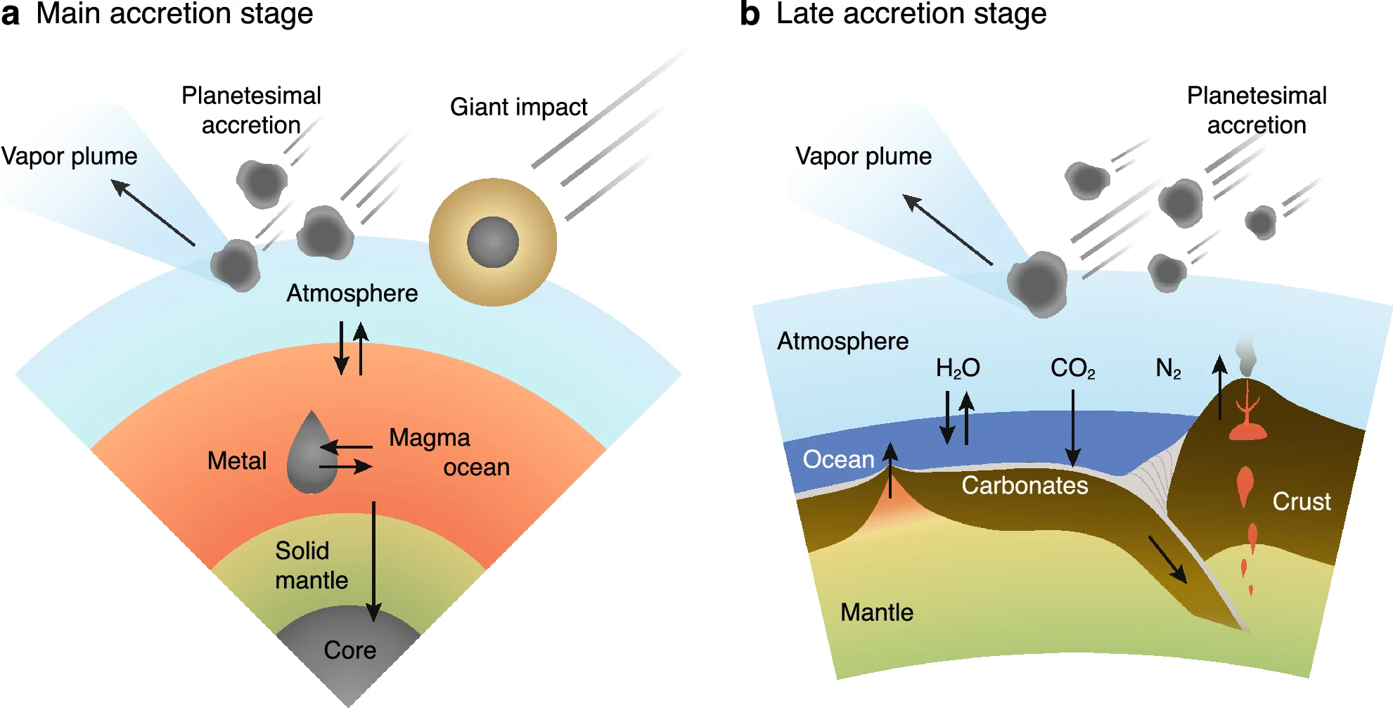
Fig. 8.3 Cartoon of element partitioning processes during Earth’s accretion, where accreting planetesimals and giant impactors deliver volatiles and simultaneously form a vapor plume eroding the atmosphere. (a) Model for the main accretion stage (10% to 99.5% of the Earth’s mass). Equilibration among the magma ocean (silicate melt), liquid metal droplets transiting to the core, and the overlying atmosphere are achieved according to each metal silicate partitioning coefficient and solubility. (b) Model for the late accretion stage after the solidification of the magma ocean (the last 0.5%). The liquid water oceans and the carbonate-silicate cycle are driven by plate tectonics on the surface. Figure Credit: Sakuraba et al. (2021).#
The early atmosphere accumulated from volcanic degassing and impacts associated with melts and metamorphic gases from hot rocks that did not melt. The major volatile gases introduced into today’s atmosphere are oxidized species (e.g., \(\rm H_2O\), \(\rm CO_2\), and \(\rm N_2\)) rather than reduced forms (e.g., \(\rm H_2\), \(\rm CO\) or \(\rm CH_4\), and \(\rm NH_3\)). The reduced/oxidized gas ratio in volcanic gases depends on the degree of oxidation in the upper mantle (i.e., the source region for the gases).
The basic composition of the upper mantle was set by \(4.4\ \rm Ga\). The heat produced by impacts during Earth’s accretion melted the planet, and molten metals (mostly iron) separated from the surrounding mixtures of silicates and oxides to sink towards the Earth’s core. Siderophile (“iron-loving”) elements segregated into the core, where some were radioactive (or the decay products of radionuclides) and provide clues about the time of core formation during the first 100 \(\rm Myr\) of Earth history. The molten mantle almost certainly contained water, where some would have dissociated into hydrogen and oxygen. If the hydrodynamic loss occurred, the overall mantle oxidation state would increase.
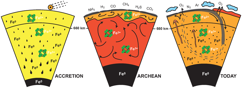
Fig. 8.4 Change in the redox state of the deep mantle. During the Earth’s accretion (left), the descending iron droplets equilibrated chemically in a partially molten mantle, which contained a major amount of bridgmanite below the 660 km discontinuity. After loss of the \(\rm Fe^0\), the lower mantle was left with a \(\rm \# Fe^{3+}\) of \({\sim}\)20 %. During the Archean (center), the oxidized deep mantle remained relatively isolated from the Earth’s surface with a tectonic regime characterized by almost no subduction. At that time, the atmosphere was anoxic. The progressive transition to modern plate tectonics around the Archean to Proterozoic Transition greatly enhanced mantle mixing (right). Figure Credit: Andrault et al. (2018).#
8.2.1. Oxygen in the Prebiotic Atmosphere#
The weakly reducing nature of volcanic emissions must have greatly limited the partial pressure of oxygen \(\rm pO_2\) in the prebiotic atmosphere because reduced gases would have dominated over the only abiotic source of free oxygen (i.e., photolysis and hydrodynamic escape). Hydrogen escape and \(\rm O_2\) production associated with water vapor destruction is severely limited because little water vapor is able to rise to the upper atmosphere due to the condensation of water at the top of the troposphere. Consequently, the abiotic production rate of \(\rm O_2\) is very small.
An oxidizing atmosphere is characterized as being “hydrogen-poor”, while a reducing atmosphere is “hydrogen-rich”. Even a small excess of \(\rm H_2\) tips the balance. Hydrogen exerts a control on the level of \(\rm O_2\) through a series of photochemical reactions that add up to a net reaction:
To estimate \(\rm pO_2\) for the prebiotic atmosphere, we assume larger outgassing rates than the modern Earth because of increased heat flow from a hotter, more radioactive interior. Assuming that \(\rm H_2\) outgassing rates were \(3-5\times\) higher, detailed photochemical models indicate that the prebiotic atmosphere’s \(\rm pO_2\) was only \({\sim}10^{-13}\ \rm bar\) (Kasting (1993))
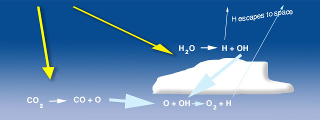
Fig. 8.5 Photolysis of \(\rm H_2O\) vapor and \(\rm CO_2\) produce \(\rm OH\) and \(\rm O_2\), respectively. Some oxygen is produced in small concentrations, while hydrogen escapes to space. Image Credit: University of Michigan#
8.2.2. The Escape of Hydrogen to Space#
The Earth did not retain gaseous volatiles from the original solar nebula, which is shown through the depletion of noble gases in Earth’s composition. As a result, Earth’s hydrogen must have been accreted from other molecular sources in solid form (e.g., water ice, water hydration in silicates \(\rm -OH\), or hydrocarbons \(\rm -CH\)). Hydrodynamic escape is important in the history of atmospheric \(\rm O_2\), where it can occur via other atmospheric gases other than \(\rm H_2O\). When hydrogen escapes to space, the Earth as a whole is irreversibly oxidized as the atmosphere becomes less hydrogen-rich. It is immaterial whether the hydrogen is transported through the atmosphere as hydrogen gas \(\rm H_2\) or any other \(\rm H-\text{bearing}\) compound. When hydrogen emanates from volcanoes, the upper mantle is oxidized through reactions such as,
The abundance of hydrogen in the atmosphere is set by a balance between \(\rm H_2\) outgassing (from volcanism and metamorphism) and escape of hydrogen to space. Hydrogen atoms are “light” (i.e., low mass and thus low inertia) so they are always some at the top of the atmosphere traveling fast enough to escape Earth’s gravity. Extreme UV radiation from the Sun is absorbed and converted into heat in the thermosphere, which has temperatures of \({\sim}1000-2500\ \rm K\). The average hydrogen thermal velocity is insufficient to achieve escape, but the high temperature thermosphere induces a high-velocity “tail” in the Maxwellian distribution of velocities. This process is called thermal escape. However, non-thermal escape mechanisms account for \(60-90\%\) of the \(\rm H\) atom escape.
There are two principal bottlenecks as hydrogen atoms work their way upwards and eventually escape. The first is the cold trap through condensation and the second is a slow diffusion process through the thermosphere. The thermosphere is analogous to a membrane with a certain partial pressure of hydrogen and a vacuum above. Calculations show that the amount of escaping \(\rm H\) today is only \(9\times 10^{10}\ \rm mol\ H/yr\) (see Kasting and Brown (1998) chapter in The Molecular Origins of Life for a detailed calculation). About half the \(H\) comes from water vapor that makes its way above the cold trap and the other half from biogenic methane. For early Earth, an outgassing rate that is \(5\times\) the modern rate can be balanced with hydrogen escape flux to space that depends on the hydrogen mixing ratio. This calculation yields a hydrogen mixing ration of \({\sim}10^{-3}\) for the prebiotic atmosphere compared to the modern value of \(5.5 \times 10^{-7}\).
8.2.3. Atmospheric Synthesis#
Reaction in the weakly reducing prebiotic atmosphere may have produced molecular precursors to life, including an early self-replicating system that led to RNA. The phosphate molecule molecule in RNA would likely be derived from phosphate released in weathering of rocks, whereas the ribose (sugar) and nitrogen in RNA might have an atmospheric origin. Ribose is \(\rm C_5H_{10}O_5\) (recall that glucose is \(\rm C_6H_{12}O_6\)), which can be formed from five molecules of formaldehyde \(\rm H_2CO\). Photochemical reactions in weakly reducing \(\rm CO_2\)-rich atmospheres are predicted to produce large quantities of formaldehyde (Pinto et al., (1980)), which is soluble and would rain out.
The simplest nitrogen-containing base is adenine \((\rm C_5H_5N_5)\), which is a chain of five hydrogen cyanide molecules (\(\rm HCN\)). Substantial \(\rm HCN\) can form in a primitive atmosphere with a few tens of ppm of \(\rm CH_4\) (Zahnle (1986)). Nitrogen atoms can be produced by ionization of \(\rm N_2\) in the ionosphere \(\rm (N_2 + \gamma \rightarrow N_2^+ + e^-)\) followed by dissociative recombination \(\rm (N_2^+ + e^- \rightarrow N + N)\). The nitrogen atoms descend into the stratosphere where they combine with fragments produced in \(\rm CH_4\) photolysis to make \(\rm HCN\):
The rate constants for these reactions and their products have not yet been studied experimentally, where there also may not have been enough prebiotic methane. Much of the methane entering today’s atmosphere is biogenic. An abiotic source of methane comes from mid-ocean ridges at a rate of \({\sim}1.5 \times 10^{10}\ \rm mol\ CH_4/yr\) and would only produce \(0.5\ \rm ppm\ CH_4\) in a weakly reducing atmosphere, or a rate of \({\sim}5.3 \times 10^{8}\ \rm mol\ CH_4/yr\). For comparison, today’s flux of micrometeorites would produce only \(1\%\) as much \(\rm HCN\) if all the nitrogen were converted to \(\rm HCN\) by heating during atmospheric entry, but the flux may have been \({\sim}100-1000\times\) higher before \(\rm 4\ Ga\).
8.3. The Oxygen Revolution#
Earth’s surface and atmosphere was transformed with the oxygen “revolution”, which was an event that started in the Archean (\({\sim}3\ \rm Ga\)) and continued into the Proterozoic. During this time, molecular oxygen levels increased, while both nitrogen and carbon dioxide levels decreased. The fundamental chemical nature of the atmosphere and its interactions with life changed drastically. Life had an active role (either principally causing or at least helping) in the increase of oxygen levels. Earth’s atmosphere is very different compared to Mars and Venus, where the carbon dioxide levels are conspicuously low.
8.3.1. The Modern Oxygen Cycle#
The Earth has many sources and sinks (losses) of oxygen, where the biosphere (land and water), volcanism, and weather contribute to the flow of oxygen in trillions of \(\rm mol/yr\) (see Fig. 8.6). The total oxygen in the atmosphere today is \({\sim}6\times 10^{17}\ \rm kg\) and is held in balance by production and loss processes.
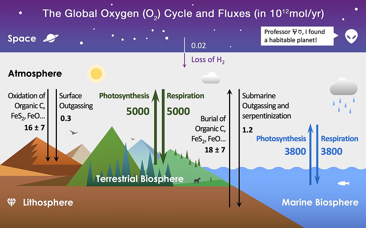
Fig. 8.6 The main reservoirs and fluxes of global oxygen cycle. Image Credit: Wikipedia:oxygen cycle.#
Here are the most important gain and loss processes, where the rates are given to the nearest order of magnitude.
Photochemistry and escape of hydrogen to space: The absorption of UV photons from the Sun by water causes photolysis (i.e., the breakup of the molecule into hydrogen and oxygen separately). The hydrogen can escape from the atmosphere, preventing recombination. The oxygen left behind makes molecular oxygen \(\rm O_2\) and ozone \(\rm O_3\). The rate of oxygen production is \(10^8\ \rm kg/yr\).
Weathering of rock: Oxygen and carbon dioxide in the atmosphere (with the help of (rain)water) attack minerals in the rock to make new compounds. Oxygen, in particular, attacks the iron in the rock that causes rusting. Estimating the rate of this process depends on how rapidly the weathered products are transported, but it is \(-10^{11}\ \rm kg/yr\), where the \(-\) sign indicates that it is a loss process.
Volcanism: Volcanoes on land and the ocean floor emit reduced gases (e.g., \(\rm CO\)) and sulfur compounds, that strongly tend to combine with oxygen in the atmosphere. The resulting rate of oxygen loss is about \(1/3\) the rate caused by weathering. Volcanoes also emit water vapor, which contributes to the source from photochemistry and escape of hydrogen to space.
Photosynthesis: Carbon dioxide is removed from the atmosphere by plants and bacteria, where oxygen is produced as a waste product. the rate of oxygen production from photosynthesis is \(\rm 10^{14}\ \rm kg/yr\).
Respiration and decay: These two processes are the reverse of photosynthesis. Oxygen is taken up from the air by animals, plants, and certain bacteria, where the oxygen is combined with sugars (or other organic compounds) to generate energy. Decay refers to organic matter that is no longer living but is consumed by microorganisms with a net loss of oxygen to generate energy. The observation that the present level of molecular oxygen is approximately constant and that respiration would deplete the atmosphere of oxygen in 6,000 years imply that respiration/decay is in balance with photosynthesis. Note that only \(3/4\) of the surface organic reservoir (in contact with the atmosphere today) is living. The total rate of oxygen loss from these process is \(\rm -10^{14}\ \rm kg/yr\).
Burial of carbon from organisms: On average, the remains of dead organisms will lie on the surface in contact with the atmosphere for several decades or more. This carbon is referred to as reduced carbon because it is relatively rich in hydrogen and tends to soak up oxygen. The primary means of burial of the reduced carbon is through deposition in continental and oceanic sediments, which breaks contact with the atmosphere and allows the carbon to be preserved. The net result is oxygen is added to the atmosphere over time because the buried carbon is no longer available to soak up the oxygen. The effective rate of production is \(10^{11}\ \rm kg/yr\).
Recycling of buried sediments: Ocean-floor sediments containing trapped carbon are recycled through the upper mantle by plate tectonics. The cycling time is \({\sim}100-200\) million years. The result is the re-emergence of reduced carbon to the surface, a net source of carbon dioxide and sink of atmospheric oxygen. The amount of oxygen loss is less than the production rate.
8.3.2. The Balance of Oxygen with Life#
A look at the numbers shows that photosynthesis is the most important source of oxygen. Respiration/decay must be the primary balancing mechanism for losing oxygen because none of the geologic processes are speedy enough to balance photosynthesis. What was the situation before life became abundant?
We can compare the most important nonbiological processes for gaining (photochemistry at \(10^8\ \rm kg/yr\)) and losing (weathering at \(\rm -10^{11}\ \rm kg\)) oxygen. Clearly, photochemistry cannot generate oxygen quickly enough to keep pace with the destruction by weathering an volcanism. Weathering and volcanism could destroy almost all of the oxygen in the atmosphere (\(6\times 10^{17}\ \rm kg\)) in \(6\) million years at its present rate. If we consider the roughly \(1\ \rm Gyr\) period before the emergence of photosynthesizing lifeforms, it becomes a sensible notion that free molecular oxygen must have been very scarce in the early atmosphere where weathering and volcanism still occurred.
8.3.3. Limits on Oxygen Levels on Early Earth#
Photosynthesis was not probably widespread during the time of the first stromatolites (\(3-3.5\ \rm Ga\)). Consequently, the rate of oxygen production was less than it is today. The early oxygen was likely absorbed by weathering and volcanic activity. Evidence for the early oxygen abundance being low and increasing significantly after \(3\ \rm Ga\) is found in a number of parts of the rock record.
Minerals unstable in the presence of oxygen: The early continental rock record (up to \({\sim}2.7\ \rm Ga\)) shows rock fragments containing pyrite and uraninite. Pyrite \(\rm FeS_2\) (in the presence of oxygen) would react so that iron oxides form. Uraninite \(\rm UO_2\) also tends to form other oxides. The presence of significant amounts of uranium in the crust was a consequence of the partial melting process that led to continent formation. The particular chemical form in which uranium exists in ancient rock tells us about the amount of free oxygen present in the atmosphere at the time the uranium was exposed to the surface (i.e., little uranium oxide \(\rightarrow\) little free oxygen). Subsequent burial of the rock ensured that these deposits would be preserved even in the presence of the modern oxygen-rich atmosphere. The presence of pyrite and uraninite suggests that the Archean and early Proterozoic atmospheres had very little molecular oxygen.
Banded iron formation: The banded iron formations (BIFs) occur commonly among sedimentary rock that are dated at \({\sim}2-3\ \rm Ga\). They are almost nonexistent in younger rocks, the exception being some dated at \(\rm 750\ \rm Ga\), possibly corresponding to a deep period of near-global glaciation. They consist of alternating dark bands containing up to \(30\%\) iron, and light bands made of silica (chert).
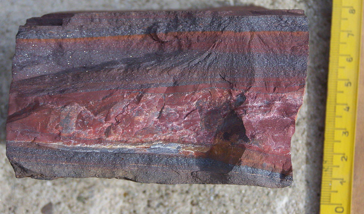
Fig. 8.7 Rock sample from a banded iron formation (BIF). Moodies Group, Barberton Greenstone Belt, South Africa. The group is dated at 3.15 Ga (billion years old). Scalebar is in cm. Sample courtesy: K. Lehmann and prof. J.D. Kramers. Image Credit: Wikipedia:Banded iron formation.#
These bands retain their distinctiveness over vast horizontal lengths (100s of \(\rm km\)). Iron must be dissolved in ocean water and deposited repeatedly on top of layers of accumulating chert on the seabed to form such bands. The sediment was compressed, which formed a hard rock over time. BIFs are found essentially on all continents and make up \({\sim}90\%\) of the world’s commercial iron supply.
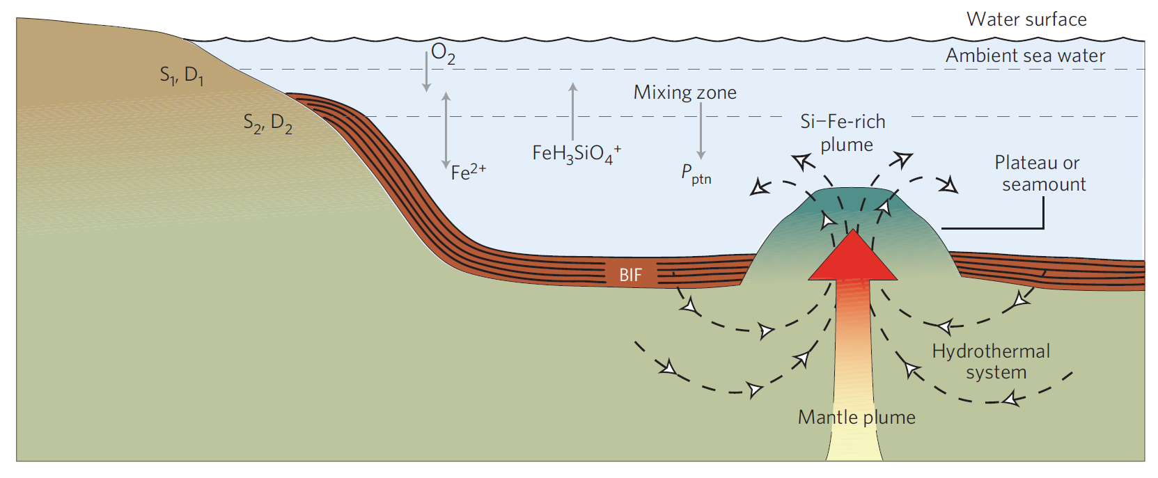
Fig. 8.8 Precipitation of BIFs from a hydrothermal system. The ambient sea water could be either oxic or anoxic. Komatiitic rocks formed as a part of plateau or seamount above a deep mantle plume. Periodic precipitation of iron oxide and silica was induced through a self-organization mechanism. \(\rm P_{ptn}\): mineral precipitation; \(\rm S_1\), \(\rm D_1\): the area of the upper surface of the mixing zone and the corresponding mass exchange coefficient for mixing respectively; \(\rm S_2\), \(\rm D_2\): the area of the lower surface of the mixing zone and the corresponding mass exchange coefficient for mixing, respectively. Figure Credit: Wang et al. (2009).#
The curiosity about BIFs lies in the need to dissolve iron in water during their formation, which cannot happen under today’s oxygen-rich atmosphere. The form of iron that dissolves in water \(\rm FeO\) is called ferrous iron. Oxygen in the atmosphere today is partly dissolved in the ocean, and can then combine with the ferrous iron to make ferric iron \(\rm Fe_2O_3\). Ferric iron is more oxidized than ferrous, where the elemental iron has bonded with more oxygen atoms than in the ferrous state. The ferric iron immediately precipitates out of the water and falls to the seafloor as iron-rich particles.
To maintain iron in the ferrous form, an atmosphere that was relatively oxygen free is required. This sets limits on the amount of oxygen in the late Archean and early Proterozoic at a few percent of the present-day value, or less. A mystery still remains: given a mechanism for dissolving the iron in the water, the production of BIFs then requires periodic precipitation of the iron out of the water. One idea suggests that the dissolved iron was contained in deep-ocean water near active vent sites. These iron-rich waters would spread by mixing over large areas fo the ocean. Upwelling of this water to the near-surface brought it into contact with regions where cyanobacteria existed, which would provide the oxygen for ferrous iron through photosynthesis.
The cyanobacteria were not the only lifeforms participating in this process. Certain other kids of “rusting” bacteria take oxygen from the surrounding environment and combine it with iron, creating stored energy usable for their life processes. This would have assisted the process of iron precipitation. The variation from sediments suggests that oxygen levels fluctuated on seasonal and longer timescales in different places at different times.
An explosion in the production rate of BIFs \({\sim}1.8-2.2\ \rm Ga\) suggests that oxygen levels worldwide had reached a threshold at which variation in the photosynthetic activity modulated the precipitation of iron from oceans. Some rare cases of BIFs occur prior to \(\rm 3\ Ga\), when worldwide oxygen levels were very low. These oldest BIFs hint that some form of photosynthesis might have occurred. Alternatively, mechanisms have been suggested by which molecular oxygen produced by atmospheric photochemistry might periodically have been concentrated in localized environments, but they remain speculative.
Redbeds: Beginning \({\sim}2\ \rm Ga\) and extending into recent times, sediments appear in the rock record that require oxygen in their formation. These redbeds form when iron is weathered out of rock in the presence of oxygen. The threshold amounts of oxygen that are required to make redbeds are significant but still small enough to permit BIFs to exist. The two overlap in the geologic record by serval hundred million years.
Fossils of aerobic organisms: Before the advent of free oxygen, organisms produced energy for biochemical processes in a number of ways. The most familiar process in anaerobic (oxygen-poor) environments is fermentation. This is where sugar is converted to ethanol and other molecules with a release of energy. The energy is stored in a biological molecule ATP. Respiration, on the other hand, uses oxygen to convert sugars to carbon dioxide and water, while producing a great deal more energy. Respiration can produce up to 36 ATP molecules from one sugar molecule. This tremendous boos in bioenergetic efficiency allowed explosive growth in the number of forms of cyanobacteria in the Proterozoic and later enabled complex cellular life.
The times at which these biological events appear in the fossil record allow the increase in oxygen in the atmosphere to be tracked. The late and relatively rapid appearance of large, complex, multicellular animals only at \(550\ \rm Ma\) suggests that oxygen levels may have remained well below the present value until then. the possibility of a dip in the molecular oxygen abundance associated with a sharp decline in plant life associated with the so-called “neoproterozoic glaciation” at \(750\ \rm Ma\) is suggested by the appearance of BIFs dating to that time. The evidence for charcoal in the fossil record between \(100-200\ \rm Ma\) implies forests capable of undergoing combustion (i.e., burning), which requires oxygen levels close to those at present (\(13\%\) compared to the present value \(21\%\)).
8.3.4. History of the Rise of Oxygen#
With the evidence for an early time of little or not atmospheric oxygen and a significant increase beginning in the Proterozoic, the amount of oxygen in the atmosphere can be tracked over Earth’s history (see Fig. 8.9).

Fig. 8.9 Main geological eons on Earth’s history, evolution of atmospheric oxygen, ocean chemistry, and occurrences of magnetofossils in the deep time. Oxygen partial pressure expressed in percent of present atmospheric level (PAL). Figure Credit: Amor et al. (2020).#
8.3.4.1. Balance between Oxygen Loss and Gain#
The rates of oxygen production and loss were different during the Archean epoch compared to the present. Biological processes were not nearly as important then, where respiration must have been negligible or nonexistent due to the absence of significant amounts of oxygen. Recycling of crust and mantle may have been much more rapid in the Archean, which led to a greater rate of volcanism. As a result, there would have been a greater flux of reduced gas in the atmosphere, which would have soaked up oxygen at a higher rate.
The change in the amount of oxygen in the atmosphere per unit time is simply the rate of production minus the rate of loss. The loss processes depend on how much oxygen is available, while the production processes do not. If we start with zero oxygen, there can be no loss of oxygen from weathering or volcanic gases. As any new source of oxygen arises, loss rates (proportional to the oxygen abundance) increase, until a new steady state is reached. Alternatively, some loss processes might saturate as the oxygen abundance rises, which would effectively increase the growth rate of the oxygen abundance. The sinks of oxygen on the early Earth must eventually have been overwhelmed by increasing rates of oxygen production.
8.3.4.2. Reservoirs of Oxygen#
The reservoirs of oxygen are offset by the substances that can soak up oxygen (e.g., via weathering, volcanism, or organic matter from near-surface, dead lifeforms). These substance are referred to as reducing compounds because they like to combine with oxygen, which reduces the amount of free oxygen. A simplified model of Earth as just atmosphere and ocean is depicted in Figure 8.10.
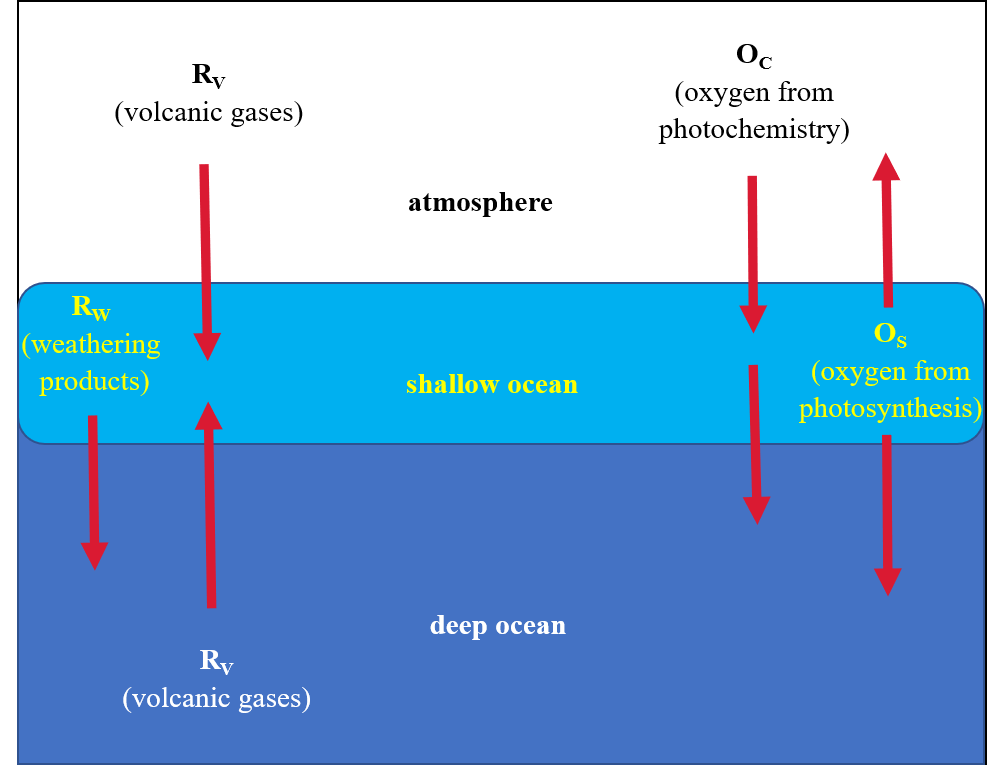
Fig. 8.10 Box model of Earth used to understand the sources “O” and sinks “R” of oxygen, where subscripts distinguish the types. The Earth is divided into three regions: atmosphere, shallow ocean, and deep ocean. Weathering products include reduced carbon from dead organisms as well as sediments, which both can soak up oxygen. Based on the model of Kasting (1991).#
Continental weathering products are ultimately deposited in the ocean, which allows us to ignore whether the volcanoes are on land or sea. The volcanic gases are present in the atmosphere or dissolved in the ocean. The deep ocean is distinguished from the shallow ocean due to the slow mixing timescale. The shallow ocean has limited contact with the atmosphere, where the deep ocean relies on convection to receive products processed at the atmosphere/shallow ocean interface. Included in the shallow are rivers and lakes.
This simplified model is a one-dimensional model, where it is useful in understanding many physical situations because of its simplicity. Obviously, there are limitations (e.g., resolving fine details) and cannot be expected to model important processes that vary from one place to another, but our information on the oxygen abundance on the early Earth is so limited that this simple model has great utility. Another limitation is the presence of the BIFs in the Archean, which indicates oxygen variations by location.
Over time, we distinguish between three states of each reservoir:
Reducing: This means that the reservoir has little oxygen and minerals (e.g., uraninite) will be stable. The iron can remain dissolved in the ocean water, which is required to produce the BIFs.
Oxidizing: The reservoir has enough oxygen to make minerals unstable and forces the iron to precipitate (i.e., removed from solution). However, not enough oxygen is available to sustain aerobic respiration.
Aerobic: Enough oxygen is present to allow aerobic respiration to occur.
8.3.5. History of Oxygen on Earth#
Based on the model in Figure 8.10, we can map the history of oxygen into four stages in Figure 8.11. The oxygen abundances in this section are represented as fractions of the present atmospheric level (PAL).

Fig. 8.11 Four stages in the history of oxygen on Earth, distinguished by oxidation state of the three major oxygen reservoirs. Important sources and sinks in each stage are shown. Based on the model of Kasting (1991).#
8.3.5.1. Stage 1#
Outgassing and impacts (carbonaceous chondrites) on the early Earth allowed for water to be established (Hadean-Archean boundary), then photochemistry begins to produce oxygen. The oxygen levels off as production is balanced by weathering and volcanism. Oxygen in the atmosphere ranges between \(10^{-5}-10^{-13}\ \rm PAL\). The range estimate considers the record in Archean sediments of the trend in abundance of the four stable isotopes of sulfur (Pavlov & Kasting (2002)). The trend follows mass independent fractionation, where it is independent of the mass differences between isotopes. This suggests that a variety of sulfur compounds (with different oxidation states) were produced photochemically in the atmosphere and preserved during their removal into sediments. BIFs from this time occur, and were formed either as solar UV radiation oxidized iron in water, or in localized environments where photosynthesizing organisms (e.g., cyanobacteria) were concentrated.
8.3.5.2. Stage 2#
The spread of oxygen-producing photosynthesizing organisms around the planet initiated a new source of oxygen. Initially, aerobic photosynthesizers would have been restricted in geographic extent. The geologic data suggest that oxygen in the atmosphere jumped to \(0.01-0.1\ \rm PAL\) around \(2-2.2\ \rm Ga\), enough to be considered oxidizing for most minerals. The geologic record for this time shows an overlap between the occurrence of BIFs and redbeds. The oxygen abundance in stage 2 is small enough that the deep ocean could have remained anoxic (reducing), whereas the shallow ocean would have been oxidizing due to photosynthetic organisms.
The steep rise in oxygen during this time period has prompted speculations on mechanisms beyond photosynthesis to pump up the atmospheric oxygen level. Geologic evidence suggests that around this time a number of small continents collided to form the first supercontinent. The assemblage of continental fragments into larger masses increased the burial rate of dead organisms (i.e., reduced carbon) as a side effect. The heightened burial rate occurred both directly in the continental interiors and on the seafloor. With less reduced carbon exposed to the atmosphere, less absorption of oxygen by these compounds could occur. Alternatively, large amounts of ocean water were mixed into the mantle by plate tectonics, which would gradually have turned the mantle from a reducing to an oxidizing chemical state. As a result, the volcanic gases became less effective in soaking up atmospheric oxygen. Either way, the elimination of oxygen sinks led to the larger growth of oxygen in the atmosphere.
8.3.5.3. Stage 3#
As photosynthesizing organisms proliferated, the oxygen abundance in the atmosphere increased. Several factors may have limited the rate of increase:
Environmental factors (e.g., near-global glaciation) could have reduced the available surface area of liquid water on the Earth. This dramatically reduces the population of oxygen-producing photosynthesizers for 100s of millions of years.
Rising oxygen levels might have provided a challenge to the defensive mechanisms against oxygen-generating free radicals within the organisms themselves. It is not too much of a fantasy to imagine that all such photosynthesizes might have poisoned themselves to the brink extinction, if not for the flexibility of an evolving genome.
The atmosphere and surface ocean reservoirs became aerobic, with the deep ocean oxidizing. BIFs could no longer be produced (except in the rare times of near-global glaciation) because iron dissolved in seawater was always unstable. The lack of iron meant that iron sulfides could no longer form, and deep ocean waters may have been sulfide rich. Redbed formations became more widespread.
8.3.5.4. Stage 4#
Eventually, the dep ocean received enough flux of oxygen to become aerobic, which ended the period of the sulfide ocean. The advent of oxygen respiration (aerobic metabolism) was initiated among lifeforms, and the number of photosynthesizing species increased. The new balance in oxygen production and loss was between photosynthesis and respiration/decay. Photochemistry, weathering, and volcanism was now insignificant in their effect on oxygen levels. The balance permitted a gradual increase in oxygen to the current abundance within the past billion years. Although there were a handful of outstanding fluctuations upward and downward due to changes in burial rates of volcanism and organic matter, as well as glacial episodes.
8.3.6. Shield against UV Radiation#
Today, the damaging short-wavelength UV photons from the Sun are shielded by ozone (\(\rm O_3\)) in Earth’s stratospheric layer. Ozone is produced photochemically from molecular oxygen by absorption of UV photons. To maintain the ozone shield, \(10^{-2}\ \rm PAL\) or higher of oxygen is required based on chemical models. Clearly, an ozone shield was not available up to \(2\ \rm Ga\).
Because UV radiation is absorbed more effectively by water than is visible radiation, photosynthesizing organisms in the oceans could have been protected from UV radiation, even at shallow depths. Other atmospheric gases and aerosols might have afforded protection from some of the UV radiation, making life on land surfaces possible. Because these shields likely were not as effective as the current stratospheric ozone layer, organisms had to develop protection themselves. Consequently, bacterial colonies form mats, which would have shielded them from the UV flux. In spite of various survival strategies, incomplete shielding of continents and the ocean’s surface from UV radiation probably restricted severely the number of viable lifeforms.
8.3.7. Onset of Eukaryotic Life#
The dramatic rise in oxygen levels around \(2\ \rm Ga\) precipitated two events that allowed for a great diversification of life, and the ecological niches that they could occupy. These were
enabling of aerobic respiration, which dramatically increased the energy that life could generate and use from the environment, and
the development of an ozone shield against ionizing UV radiation, which could damage DNA.
All aerobic cells contain enzymes that are necessary to detoxify the molecular fragments, or radicals, that contain oxygen. Without such enzymes, these free radicals would react with and destroy cellular structures. Anaerobes must avoid oxygen by existing in oxygen-poor (or reducing) environments or mounting defenses against oxygen similar to those of the aerobes. Even more intriguing, oxygen is not used in pathways for synthesizing protein and other biological molecules, but just as an energy source (with a few exceptions).
Some prokaryotes evolved to take advantage of oxygen and employ it in their metabolism. The advent of abundant oxygen in the atmosphere and ocean led to the successful spread and diversification of a new type of cell. Around \(2\ \rm Ga\), in the mid-Proterozoic, fossil evidence of eukaryotes appears, where the cellular function is divided among organelles separated by membranes. In some cases, the organelles would have their own separate DNA and RNA. The cell’s central genetic code is isolated in a nucleus, and organized into chromosomes.
Essential to the workings of the eukaryotes in the current biosphere are the plastids (e.g., chloroplasts) and the mitochondria. The plastids convert sunlight, \(\rm CO_2\), and \(\rm H_2O\) into sugars. The mitochondria take alcohols and lactic acid (products of fermentation) as inputs into a set of chemical reactions involving oxygen to create the enormous phosphate-bond storehouse of energy characteristic of aerobic metabolism.
The mitochondria and plastids provide clues to the origin of the complex eukaryotes, which both resemble bacteria. Mitochondria have their own DNA, messenger RNA (mRNA), transfer RNA (tRNA), and ribosomes (protein synthesizers) within the mitochondrial membrane. The DNA floats within the mitochondria as strands and is not bound in chromosomes. The ribosomes in mitochondria look like bacterial ribosomes, and are sensitive to the same antibiotics. Mitochondria divide at times different from the rest of the cell in a manner similar to bacteria, by simple pinching and division. Plastids resemble bacteria even more than do mitochondria in the appearance and arrangement of their internal structures.
Mitochondria and plastids cannot exist outside of their own cells, but there are plenty of examples of symbiosis among individual bacteria, and between bacteria with eukaryotes. Some eukaryotes are actually anaerobic because they lack mitochondria, but in some cases, they contain organelles specialized for fermentation. Some anaerobic eukaryotes exist in a tightly dependent relationship with other organisms (including bacteria) or actually harbor bacteria within their cells in a symbiotic relationship. Removal of the bacteria usually leads to death of the host eukaryote. Laboratory experiments have successfully forced symbiosis between bacteria and amoebas that do not normally engage in such processes of symbiosis. The experiments selected the amoebas that best accommodated the invaders, and a colony of healthy amoebas was created. The bacteria lived off the amoebas and curiously, the amoebas became dependent on the bacteria as well.
A further clue to the origin of eukaryotes lies in the predatory nature of some bacteria that will invade the cell walls of other bacteria. Although most such encounters eventually result in the death of the host, but in some cases the prey have evolved a tolerance for the predatory bacteria.
The notion that complex plants and animals, including humans, are the result of symbiotic relationships between bacteria may be shocking, but it is increasingly accepted by biologists.
The structural similarities between organelles and some bacteria,
the symbiosis between anaerobic eukaryotes and bacteria (and between different types of bacteria), and
the tolerance of some eukaryotes for forced laboratory symbiosis
all suggest that such dependencies have arisen through out the Earth’s history. Comparison of the genomes of eukaryotes and prokaryotes have led some molecular biologists to propose an earlier origin for eukaryotes (perhaps \(> 3\ \rm Ga\)).
Regardless of the original appearance of eukaryotes, their success was in the utilization of atmospheric oxygen. As cyanobacterial photosynthesis polluted the atmosphere and shallow ocean with oxygen, some bacteria (or archaea) evolved to be oxygen tolerant and then oxygen dependent. The ancestors of mitochondria were efficient enough at using oxygen that their symbiotic relationship with host bacteria created an energy-efficient, adaptable cell that would become the basis for animals and fungi. Further symbiosis brought photosynthesis into the eukaryotic realm, and plants were born. Eukaryotes spread into a variety of ecological niches, where some even adapted to survive in anerobic environments, which is in contrast to those eukaryotes that lack mitochondria and were anerobic from the start.
The advent of aerobic eukaryotes enabled predator-prey food chains to come into existence. Although these food chains existed among bacteria, the food chain is only one level: predator bacteria invade prey bacteria, and the food chain ends there. Anaerobic organisms are not efficient enough at producing energy from fermentation and other mechanisms to create enough food for a multilevel food chain, and aerobic bacteria do not come in enough morphological varieties to create such a chain themselves. Eukaryotes have the high energy efficiency and morphological diversity to sustain the multilevel food chains. Evolution toward large size and complexity is a tremendous evolutionary advantage (Fenchel & Finlay (1994)), where one can swallow smaller organisms or avoid (through size, speed, and smarts) being swallowed in turn. The high-efficiency oxygen metabolism and complex versatility of eukaryotes were prerequisites to innovations such as ourselves.