1. Overview of the Solar System

1.1. A Brief History of the Planetary Sciences

The history of the planetary sciences begins before it even had a name for it. Ancient civilizations noticed several ‘stars’ moved quickly in the night sky relative to much more numerous background stars. The Greeks called these objects πλανήτης (planētēs; wandering stars), or planets. Ancient civilizations (e.g., Chinese, Persian, Ancestral Puebloans, Maya) that developed written language and/or drawings attested to their interest in comets, solar eclipses, and other celestial phenomena. Some migratory birds (and potentially their ancestors the dinosaurs) use the patterns of stars in the night sky to guide their journeys.

The Renaissance and Enlightenment movements in western Europe (i.e., Copernican-Keplerian-Galilean-Newtonian revolution) resulted in a completely different view for the dimensions and dynamics of the Solar System. Humanity’s view of the relative sizes and masses of bodies that constitute the Solar System were drastically altered, including the forces that make them orbit one another.

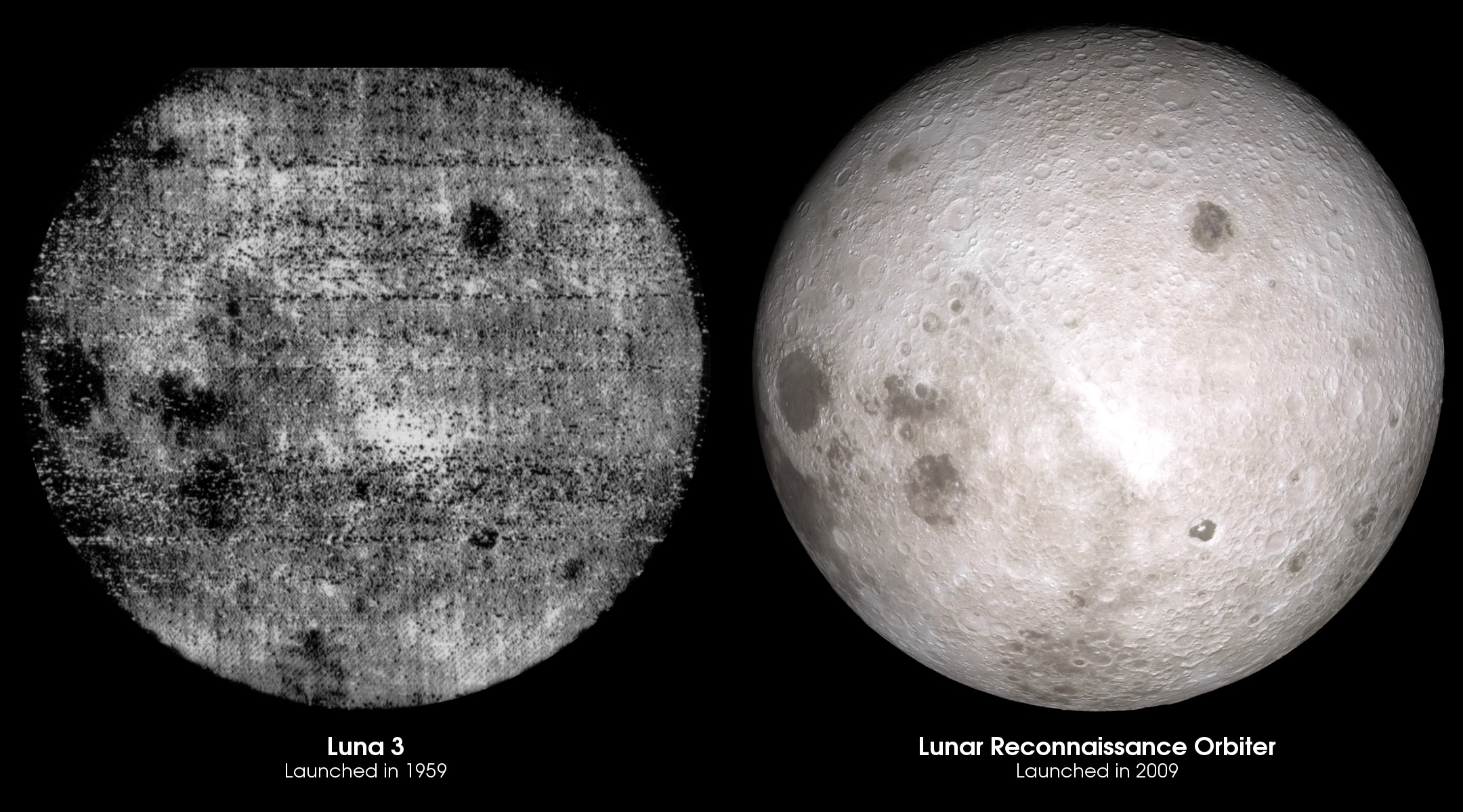
Fig. 1.1 Side by side comparison of the first ever photograph of the lunar far side, from Luna 3, and a visualization of the same view using LRO data. Image credit: NASA

The age of planetary exploration began in 1959 with the Soviet Union’s spacecraft Luna 3 (see Fig. 1.1) returning the first pictures of the farside of the Moon. During the cold war, spacecraft visited all eight known terrestrial and giant planets in the Solar System. Through spacecraft, scientists have collected data concerning the planets, their rings, and moons. This age of planetary exploration produced:

• Spacecraft images uncovered details that Earth-based pictures could not resolve.

• Spectra from across the electromagnetic spectrum (\(\gamma\)-rays to radio) revealed undetected gases and geological features on planets and moons.

• Radio detectors and magnetometers showed that other planets possessed aurorae and magnetic fields.

• Unexpected types of structure in Saturn’s rings, and whole new classes of rings (and ring systems) around all four giant planets.

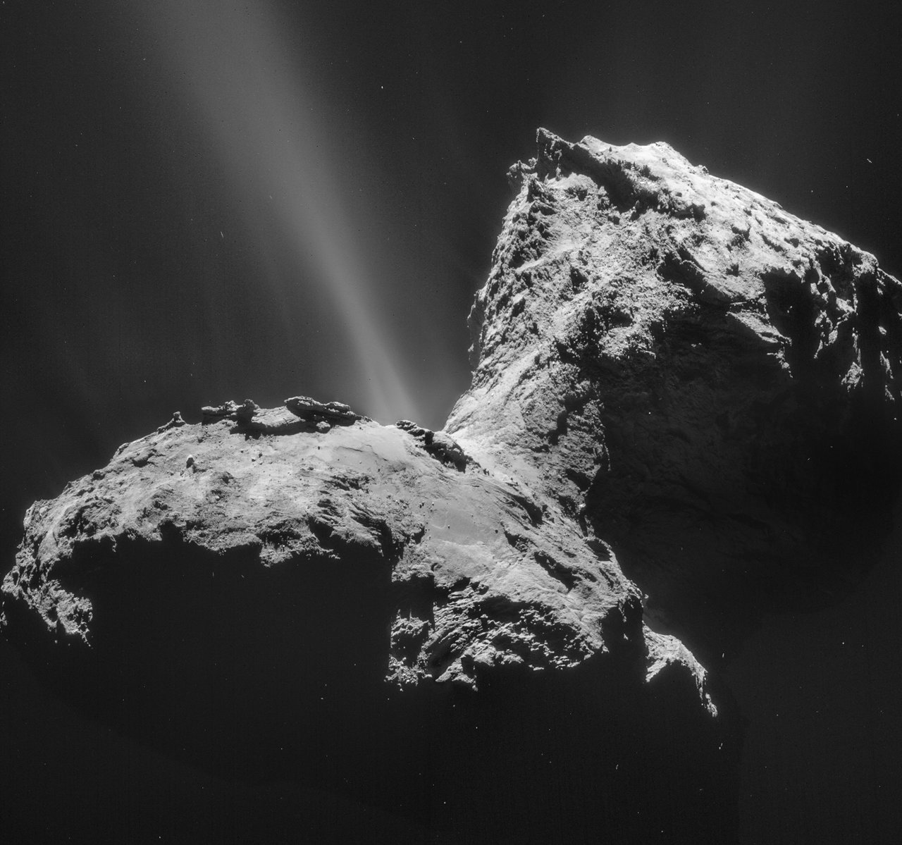
Fig. 1.2 Comet 67P/Churyumov-Gerasimenko on Jan. 31, 2015. Image credit: ESA/Rosetta/NAVCAM

Both comets and asteroids have now been explored close up by spacecraft (see Fig. 1.2). Missions have been deployed to study the Sun and its solar wind. Although the Sun’s gravitational domain extends beyond the most distant planet (Neptune), the vast outer regions of the Solar System are still poorly explored. Many small bodies are expected to be lurking in this great beyond (and some larger ones too like Planet 9), but are currently beyond our capacity to detect them.

Thousands of planets orbiting other stars (i.e., exoplanets) have been discovered by NASA’s Kepler Space Telescope and Transiting Exoplanet Survey Satellite (TESS). As you may expect, we don’t know a lot of detail concerning these exoplanets, but many of the have gross properties (e.g., orbits, masses, radii) that are quite different than any object in the Solar System. As a result, some of models of planet formation and evolution have been revised.

Biologists have redrawn the tree of life in the past few decades due to our more nuanced understanding of the relationships between Earth’s diverse lifeforms. Some species have been identified to live and thrive in extreme environments that would deadly for humans. The regions of the planet where life was considered to exist expanded, which also suggested that extreme conditions on other planets and moons in the Solar System might also be capable of sustaining life.

The planetary sciences as a subfield of astronomy has expanded to become even more interdisciplinary, where knowledge of geophysics, atmospheric science, and biology are required to develop a system-wide understanding of a planet. The properties of planets are key to astrobiology, and understanding the basics of life is useful to planetary scientists.

Fig. 1.3 Image credit: NASA

1.2. Inventory of the Solar System

• What is the Solar System?

For humans, the answer to this question starts from Earth (our home) and then progresses outwards to the things that we can readily identify. However this could be a biased view as we eventually want to find other worlds that could potentially host life. A better question is:

• What is seen by an objective observer from a huge distance?

The Solar System is then dominated by a single object, the Sun. The Sun’s energy output (luminosity) is about 400 million times larger than the Solar System’s largest planet (Jupiter). The Sun also contains nearly all the mass (\(>99.8\%\)). By these measures, the Solar System is essentially the Sun with some debris orbiting it.

If we instead measure the Solar System in terms of angular momentum, then most of it lies in the orbital motions of the planets. Moreover, the Sun is a fundamentally different type of body, where it is a ball of plasma powered by nuclear fusion in its core. The smaller bodies (i.e., debris) are composed of molecular matter. This debris is composed of giant planets, terrestrial planets, and a wide range of smaller objects that all encircle the Sun.

Fig. 1.4 Orrery showing the motions of the inner four planets of our Solar System. Distances are to scale. The circular rings are spaced 0.5 AU apart. Image credit: Wikipedia

Fig. 1.5 Orrery showing the motions of the outer four planets of our Solar System. Distances are to scale. The circular rings are spaced 4 AU apart. Image credit: Wikipedia

Figures 1.4 and 1.5 present scaled views of orbits for the inner and outer planets, respectively. The differences in scale prevent both systems from being displayed in the same figure. Figure 1.6 shows the Solar System planets scaled by size, where the terrestrial planets appear almost insignificant next to the much larger Jovian planets, Jupiter and Saturn.

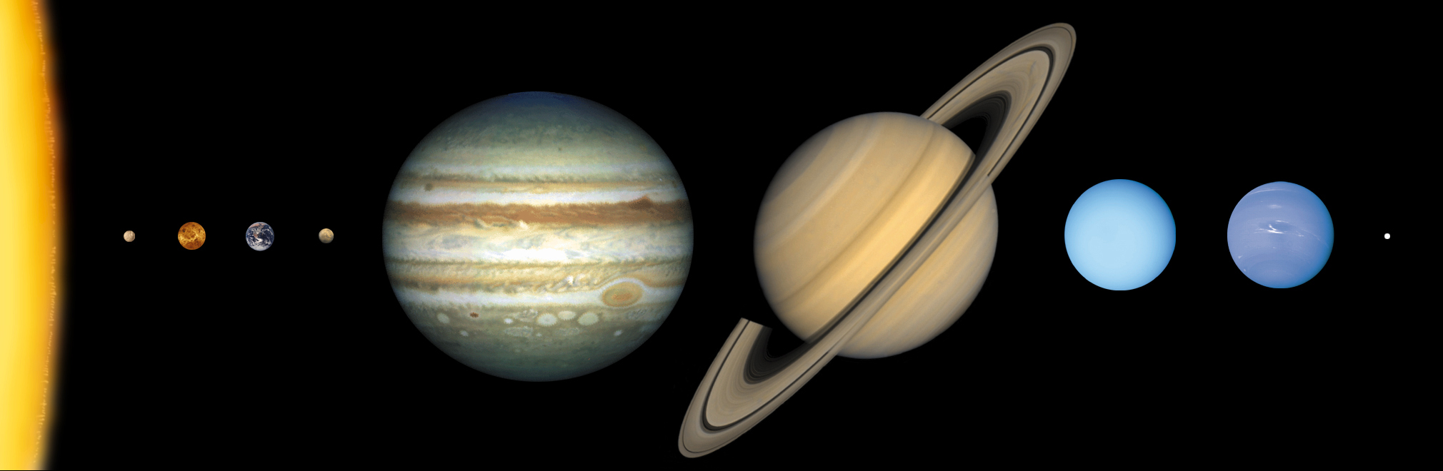
Fig. 1.6 This illustration shows the approximate sizes of the planets relative to each other. Image credit: NASA

1.2.1. Giant Planets

Jupiter dominates the planets in the Solar System in terms of both its mass (\(318\ M_\oplus\) [Earth masses] or \(9.54 \times 10^{-4}\ M_\odot\) [Solar masses]) and radius (\(11.2\ R_\oplus\) [Earth radii] or \(0.10\ R_\odot\) [Solar radii]). Jupiter has two times more mass than the remainder of the Solar System (excluding the Sun). The first approximation of the Solar System was the Sun + debris, where a second approximation would be the Sun + Jupiter + debris. The largest (in mass and radius) of the new debris category is Saturn, which is about one-third of Jupiter’s mass (\(100\ M_\oplus\)) and nearly equivalent to Jupiter’s radius (\(9.5\ R_\oplus\)). Saturn’s composition is similar to Jupiter, where they are both comprised mostly of molecular hydrogen \((\rm H_2)\) and helium \((\rm He)\). Both planets likely possess a heavy ‘core’ of \(\sim 10\ M_\oplus\).

Note

Astronomers use the term ices (or interstellar ices) to describe molecules or compounds that condense into crystals and are typically suspended within a gas cloud. Examples of water ice on Earth are snow, sleet, and hail, where astrophysical ices are more similar to snow or sleet.

Uranus and Neptune are the next largest planets, but they are much less massive (\(14\ M_\oplus\) and \(17\ M_\oplus\), respectively) and physically smaller (\(\sim 4\ R_\oplus\)) than the Jovian planets. These planets belong to a different class, with most of their masses provided by a combination of three astrophysical ices:

• water \((\rm H_2O)\),

• ammonia \((\rm NH_3)\), and

• methane \((\rm CH_4)\),

together with ‘rock’ (high temperature condensates consisting primarily of silicates and metals). Most of their volume is occupied by relatively low mass \((1-4\ M_\oplus)\) \(\rm H-He\) dominated atmospheres.

The four largest planets are known collectively as the giant planets, where they are subdivided into the gas giants (i.e., Jupiter and Saturn) and the ice giants (Uranus and Neptune). All four giant planets possess strong magnetic fields. The giant planets orbit at progressively farther distances from the Sun: 5.2 AU (Jupiter), 9.5 AU (Saturn), 19.2 AU (Uranus), and 30 AU (Neptune).

Note

One astronomical unit (1 AU) is defined as the semimajor axis of a massless (test) particle whose orbital period around the Sun is one year.

1.2.2. Terrestrial Planets

The total mass of the remaining debris (in Sun + gas giants + debris) is less than one-fifth of Uranus’ mass and their angular momenta are much smaller too. The remaining debris consists of solid bodies, that are interesting chemically, geologically, dynamically, and in the case of Earth, biologically. The two largest terrestrial planets are Earth and Venus. Venus orbits closer to the Sun (0.72 AU), is less massive \((0.82\ M_\oplus)\), and is slightly smaller \((0.94\ R_\oplus)\) than the Earth. Our Solar System contains two other terrestrial planets that are much smaller than the Earth: Mars \((0.53\ R_\oplus)\) and Mercury \((0.38\ R_\oplus)\). These terrestrial worlds are much less massive than the Earth too: Mars \((0.11\ M_\oplus)\) and Mercury \((0.06\ M_\oplus)\).

Note

In planetary science and astronomy, the word terrestrial means Earth-like or otherwise related to the Earth. Geoscientists and biologists generally use the same word to signify a relationship with land masses.

All four terrestrial planets have atmospheres, where the composition and density varies widely. Venus’ atmosphere is the thickest, while Mercury’s atmosphere is the most tenuous. Even though Venus’ atmosphere is massive by terrestrial standards, it is still miniscule compared to the giant planets. Earth and Mercury have an internally generated magnetic field. Mars’ magnetic field is extremely weak now, but it may have been stronger earlier in its history.

Exercise 1.1

To build an intuition of the size and distance differences, it is useful to use an everyday object to scale the Solar System. Assume that you can represent the Earth with a Navel orange with a 3 inch diameter.

(a) How wide would each of the planets be using this scale?

(b) The distance to the Sun (i.e., 1 AU) can be represented with approximately 11,741 Earths. How far from the Sun would you place the Earth using the Navel orange scale? Is this a practical scale to use on the Earth?

(c) How far would the other 7 planets be placed using the scale from part (b)?

---

(a) From many observations, we know the radius of each planet relative to the Earth. Therefore, we determine the scaled size using the diameter of a Navel orange (in inches) and the known relative size (in Earth radii). The following table provides the relative radius and scaled width of each planet using the Navel orange scale:

Terrestrial	Radius	Scaled Width	Giant	Radius	Scaled Width
Mercury	\(0.38\ R_\oplus\)	1.1 in	Jupiter	\(11.2\ R_\oplus\)	2.8 ft
Venus	\(0.94\ R_\oplus\)	2.8 in	Saturn	\(9.5\ R_\oplus\)	2.4 ft
Earth	\(1\ R_\oplus\)	3 in	Uranus	\(4\ R_\oplus\)	1 ft
Mars	\(0.53\ R_\oplus\)	1.6 in	Neptune	\(4\ R_\oplus\)	1 ft

(b) The distance to the Sun is given as 11,741 Earth diameters. We only need to multiply by our scale using Navel oranges to determine the distance, via

\[ d_{\rm oranges} = (11,741\ d_\oplus)(3\ \text{in}) = 35,222\ \text{in}. \]

This result is not very practical, where it would be more useful to convert from inches into miles \((1\ \text{mi} = 63,360\ \text{in})\). Then, we get

\[ d_{\rm oranges} = 35,222\ \text{in} \times \frac{1\ \text{mi}}{63,360\ \text{in}} = 0.56\ \text{mi}. \]

If the Sun were placed at VSU, then the Earth would be placed only a half mile from campus. This is a reasonable scale conceptually, and can be traveled by foot.

(c) The distance to the other 7 planets can be determined using the same procedure given in part (b), but using their respective semimajor axis in AU. The following table provides the semimajor axis and the distance using the Navel orange scale (and assuming circular orbits):

Terrestrial	\(a\) (AU)	Scaled Distance (mi)	Giant	\(a\) (AU)	Scaled Distance (mi)
Mercury	0.38	0.21	Jupiter	5.2	2.89
Venus	0.72	0.40	Saturn	9.5	5.28
Earth	1	0.56	Uranus	19.2	10.7
Mars	1.52	0.84	Neptune	30	16.7

Earth’s circumference is 24,902 miles. Using this scale, one could easily traverse the Solar System.

Note: Below is a solution that determines the values with the programming language Python.

import numpy as np

R_pl = [0.38, 0.94, 1., 0.53, 11.2, 9.5, 4., 4.]
a_pl = [0.38, 0.72, 1., 1.52, 5.2, 9.5, 19.2, 30]
pl_names = ['Mercury','Venus','Earth','Mars','Jupiter','Saturn','Uranus','Neptune'] 

Navel_orange = 3 #diameter of a Navel orange in inches
AU = 11740.533 #number of Earths in an AU

print("part a")
for i in range(0,8):
    R_i = R_pl[i]*Navel_orange
    if R_i < 12.:
        out_stg = "%s would be %1.1f inches wide." % (pl_names[i],R_i)
    elif R_i == 12:
        out_stg = "%s would be 1 foot wide." % (pl_names[i])
    else:
        out_stg = "%s would be %1.1f feet wide." % (pl_names[i],R_i/12)
    print(out_stg)

print("-------")
print("part b")
AU_oranges = Navel_orange*AU #scaled AU in inches
AU_oranges /= 63360. #scaled AU in miles
print("Using the Navel orange scale, 1 AU is equal to %1.2f miles." % np.round(AU_oranges,2))

print("-------")
print("part c")
print("Using the Navel orange scale:")
for i in range(0,8):
    d_i = a_pl[i]*AU_oranges
    print("%s is %1.2f miles from the Sun." % (pl_names[i],np.round(d_i,2)))

part a
Mercury would be 1.1 inches wide.
Venus would be 2.8 inches wide.
Earth would be 3.0 inches wide.
Mars would be 1.6 inches wide.
Jupiter would be 2.8 feet wide.
Saturn would be 2.4 feet wide.
Uranus would be 1 foot wide.
Neptune would be 1 foot wide.
-------
part b
Using the Navel orange scale, 1 AU is equal to 0.56 miles.
-------
part c
Using the Navel orange scale:
Mercury is 0.21 miles from the Sun.
Venus is 0.40 miles from the Sun.
Earth is 0.56 miles from the Sun.
Mars is 0.84 miles from the Sun.
Jupiter is 2.89 miles from the Sun.
Saturn is 5.28 miles from the Sun.
Uranus is 10.67 miles from the Sun.
Neptune is 16.68 miles from the Sun.

1.2.3. Minor Planets and Comets

The Kuiper belt consists of a thick disk of small bodies beyond the orbit of Neptune. These bodies are composed of a mixture of ice and rock, where the two largest members are Eris and Pluto. These Kuiper belt objects (KBOs) have eccentric orbits, which means that their heliocentric distance oscillates over a single orbit. Eris lies between \(38-97\ \rm AU\), while Pluto’s distance varies between \(29-50\ \rm AU\). The radii of Eris and Pluto are greater than 1000 km \((\sim 0.18\ R_\oplus)\). On July 14 2015, the New Horizons space probe characterized Pluto’s atmosphere, although it was known to have an atmosphere since the 1980s. Many other KBOs have been cataloged, but the census of these objects is still incomplete.

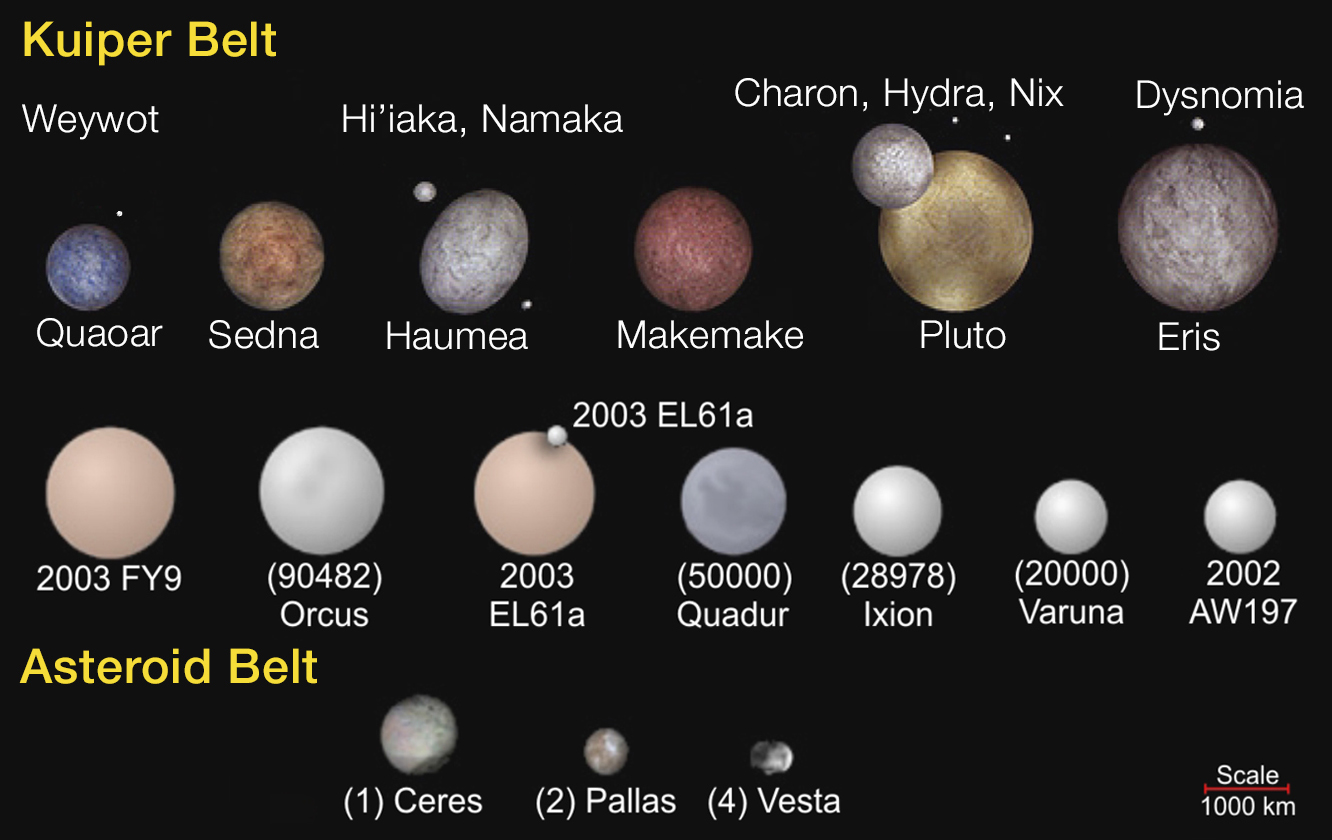
Fig. 1.7 This illustration shows the approximate sizes of objects in the Kuiper and Asteroid belts. Image credit: NASA/JHU/APL

A minor planet directly orbits the Sun. It is neither a planet nor exclusively classified as a comet. Minor planets include asteroids (i.e., near-Earth objects, Mars-crossers, main-belt asteroids, and Jupiter trojans), as well as distant minor planets (centaurs and trans-Neptunian objects). As of June 2021, there are 1,086,655 known objects, divided into 567,132 numbered (secured discoveries) and 519,523 unnumbered minor planets, with only five of those officially recognized as a dwarf planet.

Comets are ice-rich objects (i.e., dirty snowballs) that shed mass when subjected to solar heating (inside of Jupiter’s orbit). Comets may have formed near the giant planet region initially, but were transported and stored in the Oort Cloud, Kuiper Belt, or the scattered disk. The Oort cloud is a nearly spherical region that extends to \(\sim 10^4\ \rm AU\). Scattered disk objects (SDOs) have moderate to high eccentricity orbits that lie wholly (or at least partially) withing the Kuiper belt. The total number of comets (larger than 1 km in radius) in the entire Oort cloud is estimated to range from \(\sim 10^{12}-10^{13}\). The total number of KBOs of a similar size is estimated to be \(\sim 10^8-10^{10}\).

The smallest bodies known to orbit the Sun have been observed collectively, but not yet individually detected, via remote sensing. Dust grains that together produce the faint band in the planet orbital plane are known as the zodiacal cloud.

1.2.4. Satellite and Ring Systems

Beyond those bodies orbiting the Sun are some of the most interesting objects in the Solar System, which in turn orbit the planets. Two of the planetary satellites (Jupiter’s moon Ganymede and Saturn’s moon Titan) are slightly larger than the planet Mercury. These bodies are half as massive as Mercury, where a large portion of their mass is dominated by ices. Titan’s atmosphere is about four times denser than Earth’s atmosphere. Neptune’s moon Triton has an atmosphere that is much less dense, but it has powerful winds that strongly perturb particles ejected from geysers on its surface. Very tenuous atmospheres have been detected on the Moon (Earth’s satellite), Io (Jupiter’s satellite), and Enceladus (Saturn’s satellite).

Natural satellites orbit most of the planets in the Solar System (only Mercury and Venus are without natural satellites). Even KBOs and asteroids can have natural satellites. The giant planets have large satellite systems consisting of moons of many sizes and rings. Most of the smaller moons were discovered from spacecraft flybys. All major satellites (except Triton) orbit in the direction of the host planet’s rotation (i.e., prograde) and close to the planet’s equatorial plane. Small close-in moons also inhabit low-inclination, low-eccentricity orbits, but small, distant moons can travel around the planet in the direction opposite of the planet’s rotation (i.e., retrograde) as well as prograde. Moreover, such moons are often in highly inclined and eccentric orbits.

Fig. 1.8 Selected moons, with Earth to scale. Nineteen moons are large enough to be round, and one, Titan, has a substantial atmosphere. Image credit: Wikipedia:natural satellites

Earth and Pluto each have a satellite that is very massive compared to the host planet. Our Moon is about 1.67% of Earth’s mass, where Charon is about 10% of Pluto’s mass. These moons aer suspected to have been produced through giant impacts when the Solar System was much younger. Two tiny moons (Phobos & Deimos) travel on low-inclination, low-eccentricity orbits around Mars. Current models suggest that Phobos will eventually (in millions of years) fall towards Mars and disrupt to form a planetary ring.

The four giant planets all have ring system, which are primarily located within about 2.5 \(R_p\) (planetary radii) from the planet’s center. The character of each ring system varies greatly, where Saturn’s rings are bright, broad, and full of structure (such as density waves, gaps, and spokes). Jupiter’s ring is very tenuous and mostly consists of small particles. Uranus has nine narrow, opaque rings and broad dust regions orbiting in the planet’s equatorial plane. Neptune has four rings (two narrow and two broad), where the narrow rings have bright segments called ring arcs.

1.2.5. Heliosphere

All planetary orbits lie within the region of space containing the Sun’s magnetic fields and ionized gas called the heliosphere. The solar wind consists of ionized gas (i.e., plasma) that travels outward from the at high speed (\(\sim 400\ {\rm km/s}\)). The solar wind merges with the interstellar medium (ISM) at the boundary of the heliosphere called the heliopause. Three interstellar probes (Voyager 1, Voyager 2, and Pioneer 10) are currently beyond the heliopause.

The composition of the heliosphere is dominated by protons and electrons from the solar wind, where there are about \(5 \times 10^6\ {\rm protons/m^3}\) that intersect Earth’s orbit at 1 AU. The density of the solar wind decreases following an inverse square law (\(\rho \propto 1/r^2\)). The solar wind reaches \(\sim 400\ {\rm km/s}\) near the Sun’s equatorial plane, but its speed increases to \(\sim 800\ {\rm km/s}\) closer to the poles.

Fig. 1.9 This illustration shows the position of NASA’s Voyager 1 and Voyager 2 probes, outside of the heliosphere, a protective bubble created by the Sun that extends well past the orbit of Pluto. Image credit: Wikipedia:heliosphere

The local ISM consists of mainly \(\rm H\) and \(\rm He\), with a density of \(< 1\times 10^5\ {\rm atoms/m^3}\). The Sun’s motion relative to its neighboring stars is about \(18\ {\rm km/s}\), where the heliosphere also moves through the ISM at this speed (i.e., Galilean relativity). When medium A travels through another (less dense) medium B, the shape of medium A can conform into a teardrop with a tail in the downwind direction. This happens on Earth for raindrops falling through the atmosphere. The heliosphere is believed to be shaped in a similar way as it moves through the ISM. Interstellar ions and electrons generally flow around the heliosphere because they cannot cross the solar magnetic field lines. Neutral atoms can enter the heliosphere, where the \(\rm H\) and \(\rm He\) atoms from the ISM move in the downstream direction with a speed of \(\sim 15-20\ {\rm km/s}\).

The solar wind is slowed at a boundary just interior to the heliopause called its termination shock. The location of this shock moves radially with respect to the Sun in accordance with the 11-year solar activity cycle and variations in the solar wind pressure. The region between the termination shock and the heliopause is called the heliosheath.

1.3. What is a Planet?

The ancient Greeks referred to all moving objects in the sky as planets, where there were seven such objects (Sun, Moon, Mercury, Venus, Mars, Jupiter, and Saturn). The Copernican revolution removed the Sun and Moon as planets, but added the Earth. Uranus and Neptune were discovered in the 18th and 19th centuries, respectively, with the aid of the telescope.

The next ‘planet’ discovered after Uranus was 1 Ceres (the largest member of the asteroid belt) in 1801. Shortly after there were several other similar-sized bodies 2 Pallas (in 1802) and 4 Vesta (in 1807) orbiting at nearly the same distance from the Sun. It became clear that these were not planets in the same sense as the previously discovered planets and were later called asteroids. Pluto was discovered by Clyde Tombaugh in 1930 and was initially believed to Earth-like in mass and radius. More observations revealed that is actually much smaller (and less massive) than the Earth and orbits along with many other similar sized objects (i.e., Eris and other KBOs). In 2006, Pluto was reclassified as a dwarf planet by the International Astronomical Union (IAU). The IAU made the following resolution for the definition of a planet and dwarf planet:

• planet: A celestial body that (1) orbits the Sun, (2) has sufficient mass to assume a (nearly round) shape through its self-gravity, and (3) has cleared its orbital neighborhood of similar sized-bodies.

• dwarf planet: A celestial body that (1) orbits the Sun, (2) has sufficient mass to assume a (nearly round) shape through its self-gravity, (3) has not cleared its orbital neighborhood of similar sized-bodies, and (4) is not a satellite.

Detections of other substellar object orbiting other stars have raised a similar question concerning the size limit for planethood. The current IAU nomenclature for range between a planet and star are:

• Star: self-sustaining (proton; \(\rm ^{1}_1H\)) fusion is sufficient for thermal pressure to balance gravity. For solar composition, the minimum mass for an object to be a star is \(\sim 0.075\ M_\odot\) (or \(\sim 79\) Jupiter masses) and is referred to as the hydrogen burning limit.

• Stellar remnant: no more fusion (i.e., dead star), where the object is no longer supported by thermal pressure.

• Brown dwarf: substantial deuterium (proton + neutron; \(\rm ^{2}_1H\)) fusion , where more than of the object’s original deuterium inventory is destroyed by fusion.

• Planet: negligible fusion, with a precise mass limit depending on the initial composition (\(\lesssim 0.012\ M_\odot\)). It can orbit one (or more) stars, a stellar remnant, or no stars at all (i.e., rogue planet).

1.4. Planetary Properties

All of our knowledge regarding specific characteristics of Solar System objects is ultimately derived from observations, which can be astronomical measurements from the ground, Earth-orbiting satellites, or from close-up (i.e., in situ) measurements from spacecraft. With the help of various theories, the observations can be used to constrain planetary properties, such as bulk composition and interior structure. These are also crucial elements necessary for modeling the formation of the Solar System.

1.4.1. Orbit

By 1615 Johannes Kepler deduced three laws of planetary motion from observations:

1. All planets move along elliptical paths with the Sun at one focus.

2. A line segment connecting any given planet and the Sun sweeps out area at a constant rate (i.e., equal area in equal time).

3. The square of a planet’s orbital period \(P_{\rm orb}\) is proportional to the cube of its semimajor axis \(a\) (i.e., \(P_{\rm orb}^2 \propto a^3\)).

A Keplerian orbit is uniquely defined by six orbital elements in a coordinate system, where the major axis of the ellipse is parallel to the \(y\)-axis

• semimajor axis \(a\): half the length of the long (major) axis of the ellipse.

• eccentricity \(e\): the fraction by which a focus is displaced distance \(d\) from the center of the ellipse \((e = d/a)\).

• inclination \(i\): an angle that rotates the orbit about the \(x\)-axis.

• argument of pericenter \(\omega\): an angle that rotates the orbit about the \(z\)-axis. It also helps locate the eccentricity vector \(\vec{e}\).

• longitude of ascending node \(\Omega\): an angle that rotates the orbit about the \(z\)-axis. It also helps locate the inclination vector \(\vec{i}\).

• true anomaly \(f\): an angle that begins at the pericenter and rotates along the orbit to locate the planet at a given epoch.

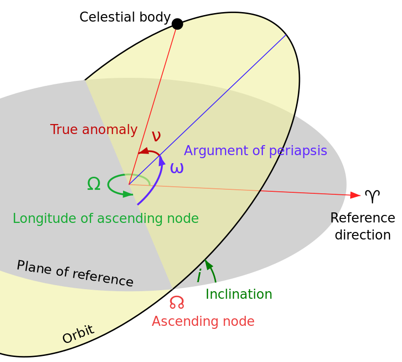
Fig. 1.10 Illustration of a Keplerian orbit, where the reference direction is along the \(y\)-axis. The true anomaly is denoted by the greek letter \(\nu\). Image credit: Wikipedia:Kepler Orbit by User:Lasunncty.

The first two elements (\(a\) and \(e\)) define the shape of the ellipse, where the elements \(i\), \(\omega\), and \(\Omega\) are angles that rotate the ellipse about the respective axes (see Fig. 1.10). The true anomaly defines where the planet is located along the ellipse, and is sometimes denoted by the greek letter \(\nu\). An alternative angle called the longitude of pericenter or varpi is simply the sum of the argument of pericenter with the longitude of ascending node for prograde orbits (i.e., \(\varpi = \omega + \Omega\)). For retrograde orbits, varpi is defined as the difference between the respective angles.

Alternative sets of orbital elements are also possible. For example, an orbit is fully specified by the planet’s Cartesian location and velocity relative to the Sun at a given time (epoch), which requires six independent scalar quantities, provided the masses of the Sun and the planet are known.

Kepler’s laws can be derived from Newton’s laws of motion and gravity that were developed in the 17th century. In most instances, this is sufficient where corrections (through General Relativity) to Newton’s laws are necessary when a planet orbits sufficiently close to the Sun. Otherwise, planetary orbits can be modeled using classical methods that account for the gravitational perturbations between planets and the gravitational force exerted by the Sun.

All planets and asteroids revolve around the Sun in the direction of solar rotation. Their orbital planes generally lie within a few degrees of each other and are close to the solar equator. For observational convenience, inclinations are usually measured relative to the Earth’s orbital plane (i.e., the ecliptic plane). The Sun’s equatorial planet is tilted by \(7^\circ\) from the ecliptic. Mercury’s orbit is also tilted \(7^\circ\) from the ecliptic, but it is tilted \(3.4^\circ\) from the Sun’s equatorial plane due to its ascending node and the spherical law of cosines. The other major planets all lie nearly in the plane of the ecliptic. Most major satellites also orbit within their host planet’s equatorial plane. Some comets and satellites orbit opposite to the Sun’s or planet’s rotation (i.e., retrograde).

1.4.2. Mass

The mass of an object can be deduced from the gravitational force that it exerts on other bodies through the following:

• Orbits of moons: The orbital periods of natural satellites and Newton’s generalization of Kepler’s 3rd law can be applied to determine the mass of the host planet \(M_p\). The result is actually the sum of the masses between the planet and satellite, but to a first good approximation it represents the planet mass (i.e., \(M_p \approx M_p + M_{\rm sat}\)). For massive moons (e.g., Earth/Moon or Pluto/Charon), the approximation breaks down and other methods are needed. The major source of uncertainty in this method lies in measurement errors in the semimajor axis, where timing errors are negligible.

• Gravitational perturbations: The gravity of planetary neighbors is sometimes sufficient to allow for a mass measurement. The accuracy for this method is not as high because of the large distances involved. The timing differences on the observed body has been used to discover and confirm a host of exoplanets. Additionally, Neptune was discovered using variations in the motion of Uranus.

• Spacecraft tracking: The motions of planets and moons can be identified through the Doppler shift in a radio signal, which correlates to the mass of each body very precisely. The long time baselines from orbiter missions allow much higher accuracy than for flyby missions. Some of the outer planet moons were measured by flyby measurements with the Voyager tracking data.

• Spiral density waves: The masses of Saturn’s inner moons can be derived from the amplitude of spiral density waves resonantly excited within Saturn’s rings.

• Nongravitational forces: The masses of some objects can be crudely estimated by the asymmetric escape of gas and dust, where this affects the observed orbit.

The gravity field of a non-spherically symmetric mass distribution differs from a point source of identical mass. Such deviations can be used to estimate the degree of central mass concentration in rotating bodies, if the rotation period is well known. This effect is most pronounced for points close to the rotating body. One can make use of spacecraft tracking data and the orbits of moons/rings to determine the precise gravity field.

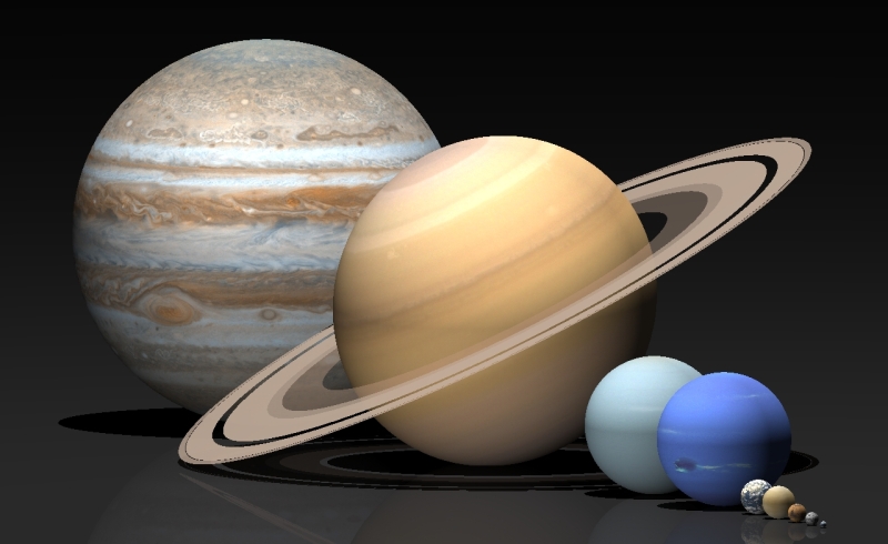
Fig. 1.11 Rendering of the Solar System planets (and Pluto) scaled by size using a computer program called Pov-Ray. Image credit: Dan Bruton:midnightkite.com.

1.4.3. Size

Bodies in the Solar System occur in a broad range of shapes and sizes. The planets are nearly round (see Fig. 1.11), but asteroids and comets come in a wider variety of shapes (e.g., potato and dog-bone). The size of an object can be measured in various ways:

• Angular size and Distance: The diameter of a body \(d_b\) is the product of its angular size \(\theta\) (in radians) with its distance \(d_o\) from the observer (i.e., \(d_b \approx d_o\theta\)). Solar System distances are simple to estimate from orbits (via parallax). The limited resolution from ground-based observations results in large uncertainties in angular size. For bodies below this resolution limit, it is better to measure the size at close distances by interplanetary spacecraft.

• Occultation: The diameter of a body can be deduced by observing a background star that is being blocked (i.e., occulted) by the body in the foreground. The angular velocity \(\dot{\theta}\) of the star relative to the body can be calculated using orbital data (after accounting for observational effects of Earth’s orbit and rotation). An estimate for the distance across a body (i.e., a chord) can be determined by measuring the duration of the occultation \(\Delta t_{occ}\), and then multiplying by the angular velocity and distance (i.e., \(d_b \approx \dot{\theta} \Delta t_{occ} d_o\)). Three well-separated chords are sufficient for a spherical planet, but many chords are needed if the body is irregularly shaped. This technique is useful for small bodies and requires an intense amount of planning to obtain enough chords.

• Radar: Similar to mapping the ocean floor or identifying aircraft, the echoes of a wave can be used to determine radii and shapes. The signal strength of radar drops as \(1/r^4\) because it falls as \(1/r^2\) on the outgoing trip and \(1/r^2\) again on the return trip. This limits this technique to relatively nearby objects, such as solid planets, asteroids, and cometary nuclei.

• Lander and Orbiter: An excellent way to measure the radius is through the use of a lander and orbiter using triangulation. This method works well for terrestrial planets and satellites with substantial atmospheres (e.g., Titan).

• Photometric Observations: The reflection of light (i.e., albedo) at visible and infrared (IR) wavelengths can be used to measure the size. The resulting lightcurve from these observations can be numerically modeled to determine its shape. Variations of this method have been used to measure the sizes for 1000s of exoplanets.

The mean density \(\rho\) of an object can be trivially determined after both the mass and size are measured (i.e., \(\rho = \text{mass}/\text{volume}\)). The density of an object gives a rough idea of its composition, although compression at high pressures must also be taken into account or the possibility of significant voids. The low density \(\sim 0.6-1.7\ {\rm g/cm^3}\) of the four giant planets implies material with low mean molecular weight. Terrestrial planet densities \((\sim 3-5.5\ {\rm g/cm^3})\) imply rocky material including silicates and some metal. Most of the medium-large satellites orbiting giant planets have low densities \((1-2\ {\rm g/cm^3})\), which implies a combination of high density rock with low density ice; recall the density of water is \(1\ {\rm g/cm^3}\) and water ice is \(0.917\ {\rm g/cm^3}\). Comets have densities nearly equal to water ice.

The escape velocity can be determined using the mass and size of an object. The escape velocity and temperature can be used to estimate a planetary body’s ability to retain an atmosphere. Both of these effects are related to measuring a planet’s gravity.

1.4.4. Rotation

Rotation is a vector quantity (having a magnitude and direction) that is related to the spin angular momentum. The obliquity (or axial tilt) of a planetary body is the angle between its spin and orbital angular momentum (see Fig. 1.12). A body with an obliquity \(<90^\circ\) is defined to have a prograde rotation (i.e., the spin and orbit are along the same direction), where as a retrograde body has an obliquity \(>90^\circ\). Note that these terms are not to be confused with prograde or retrograde orbits.

Fig. 1.12 Description of relations between Axial tilt (or Obliquity), rotation axis, plane of orbit, celestial equator and ecliptic. Earth is shown as viewed from the Sun; the orbit direction is counter-clockwise (to the left). Image credit: Wikipedia:Axial Tilt by Dennis Nilsson.

The rotation of an object can be determine using various techniques:

• Surface Markings: The most straightforward method to determine a body’s rotation axis and period is to observe how markings on the surface move around with the disk. Such markings can include uniquely sized or shaped impact craters; persistent cloud formations; or starspots (i.e., magnetic field interactions with a plasma). Not all planets have such features (e.g., Venus). If atmospheric features are used, winds may cause the deduced period to vary with latitude, altitude, and time.

• Magnetic Fields: Bodies with sufficient magnetic fields trap charged particles within their magnetospheres. These charged particles are accelerated by electromagnetic forces and emit radio waves. The radio signals have a periodicity that is equal to the rotation of the planet. For planets without solid surfaces, the magnetic field period is viewed as more fundamental than the periods measured with clout features.

• Photometric Observations: The brightness variations of an object is measured as a lightcurve (i.e., total disk brightness as a function of time). The variations can be the result of differences in albedo or projected area (for irregularly shaped bodies). Most asteroids have double-peaked lightcurves, indicating that the variations are due to the shape.

• Doppler Shifts: The measured Doppler shift across the disk can give a rotation period and a crude estimate of the rotation axis, if the body’s radius is known. This can be done passively in visible light, or actively using radar.

The rotation periods of most objects orbiting the Sun range from \(3\) hours to a few days. Mercury and Venus form exceptions with periods of 59 and 243 days, respectively, and are partially explained by the slowing effect of solar tides. Most Solar System planets (6 out of 8) rotate in a prograde sense with a respective obliquity that is \(\leq 30^\circ\). Venus and Uranus rotate in a retrograde direction with an obliquity of \(177^\circ\) and \(98^\circ\), respectively. Most planetary satellites rotate synchronously with their orbital periods (i.e., \(P_{\rm orb} \approx P_{\rm rot}\)) as a result of planet-induced tides. For a satellite to always face the central body (e.g., the Moon around the Earth), it must rotate. Otherwise, the whole surface is exposed to the central body (see Fig. 1.13).

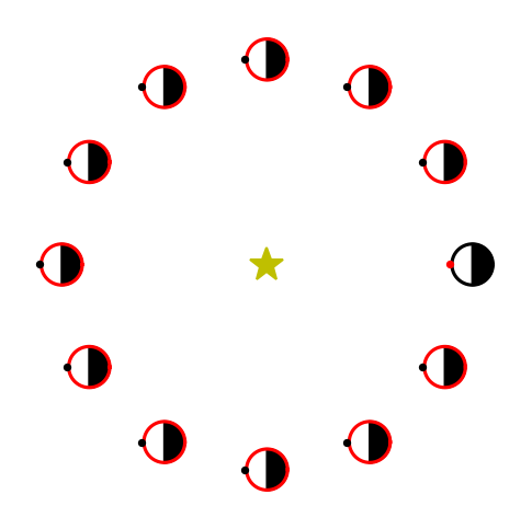
Fig. 1.13 A non-rotating planet orbiting a star, where the solid (black) circle denotes the initial position and the red dot marks a point on the surface. The solid (red) circles with black dots correspond to positions along the orbit advanced in \(30^\circ\) increments. Note that the point is no longer facing the central star halfway through the orbit.

import numpy as np
import matplotlib.pyplot as plt
from matplotlib.patches import Wedge
from myst_nb import glue

def rotate(x,y,theta):
    xp = x*np.cos(theta) - y*np.sin(theta)
    yp = x*np.sin(theta) + y*np.cos(theta)
    return xp, yp

theta_ang = np.arange(0,2.*np.pi,0.01)
half_idx = int(len(theta_ang)/2)

orb_semi = 0.1
orb_x, orb_y = rotate(orb_semi,0,theta_ang) 

cir_r = 0.01
cir_x, cir_y = rotate(cir_r,0,theta_ang)
lw = 1.5
ms=5

fig = plt.figure(figsize=(4,4),dpi=150)
ax = fig.add_subplot(111)

ax.plot(0,0,'*',color='y',ms=15)
#ax.plot(orb_x,orb_y,'-',color='b',lw=1)

ax.plot(cir_x + orb_x[0],cir_y+orb_y[0], 'k-',lw=lw)
w1 = Wedge((orb_x[0],orb_y[0]), cir_r, 270, 90, fc='black', edgecolor='black')
ax.add_artist(w1)
ax.plot(cir_x[half_idx] + orb_x[0]-0.001,cir_y[half_idx]+orb_y[0],'.',color='r',ms=ms)

#advance in orbit in increments of 30 degrees
for i in range(1,12):
    orb_x, orb_y = rotate(orb_semi,0,theta_ang+i*np.radians(30))
    w1 = Wedge((orb_x[0],orb_y[0]), cir_r, 270, 90, fc='black', edgecolor='black')
    ax.add_artist(w1) 
    #cir_x, cir_y = rotate(cir_r,0,theta_ang+i*np.radians(30))
    ax.plot(cir_x + orb_x[0],cir_y+orb_y[0], 'r-',lw=lw)
    ax.plot(cir_x[half_idx] + orb_x[0]-0.001,cir_y[half_idx]+orb_y[0],'.',color='k',ms=ms)

ax.set_aspect('equal')
ax.axis('off')
glue("nonrot_fig", fig, display=False);

1.4.5. Shape

Many different forces together determine the shape of a body. Self-gravity tends to produce bodies of a spherical shape, which is a consequence of a minimum for gravitational potential energy. Material strength maintains shape irregularities, which are produced by accretion, impacts, or internal geological processes. Bodies with mean radii larger than \(\sim 200\ {\rm km}\) are fairly round, and smaller objects may be quite oddly shaped. Figure 1.14 shows the nonspherical shape of Mars’ moon Phobos through a solar eclipse caught by the Perseverance rover.

Fig. 1.14 NASA’s Perseverance Mars rover used its Mastcam-Z camera system to shoot video of Phobos, one of Mars’ two moons, eclipsing the Sun. It’s the most zoomed-in, highest-frame-rate observation of a Phobos solar eclipse ever taken from the Martian surface. Image credit: NASA/JPL-Caltech/ASU/MSSS/SSI.

A relationship exists between a body’s rotation and its oblateness (i.e., flatness). The rotation introduces a centrifugal psuedo-force that causes the planet to bulge out at the equator and flatten at the poles. A perfectly fluid planet would be shaped as an oblate spheroid. Polar flattening is greatest for planets that have a low density and rapid rotation. In the case of Saturn, the flattening parameter \(\epsilon\) is calculated using the equatorial \(R_{\rm eq}\) and polar \(R_{\rm pol}\) radii as

\[ \epsilon \equiv \frac{ R_{\rm eq}- R_{\rm pol}}{ R_{\rm eq}} \sim 0.1. \]

The shape of an object can be determined from:

• Direct Imaging: Photographic images taken from the ground or spacecraft with an appropriate plate scale.

• Chord Lengths: Stellar occultation experiments can provide the estimates of the chord lengths (see Sect. 1.4.3).

• Radar Echoes: Reflections and/or diffraction of radio waves can provide vertices necessary for a shape model.

• Lightcurves: Several lightcurves obtained from different viewing angles are required for accurate measurements. It is similar to Radar echoes, but in at visible or IR wavelengths.

• Central Flash: When the center of a body with an atmosphere passes in front of an occulted star, the central flash results from the focusing of light rays refracted by the atmosphere and can only be seen under fortuitous observing circumstances.

1.4.6. Temperature

The equilibrium temperature of a planet can be estimated from the energy balance between the incoming solar radiation (i.e., insolation) and the outgoing long-wave radiation back into space. Internal heat sources provide a significant contribution to the energy balance of many planets. Daily (diurnal), latitudinal, and seasonal effects can induce temperature variations. The greenhouse effect raises the surface temperature on some planets far above the equilibrium temperature, where the atmosphere behaves like a thermal ‘blanket’ that is more transparent to visible radiation and prevents the escape of longer-wavelength infrared (IR) radiation.

Fig. 1.15 Earth’s energy budget describes the balance between the radiant energy that reaches Earth from the sun and the energy that flows from Earth back out to space. Image Credit: NASA.

The thermal IR spectrum of a body’s emitted radiation is also a good indicator of the temperature of its surface or cloud tops. Most solid and liquid planetary material can be characterized as a nearly perfect blackbody with an emission peak in the near- to mid-IR wavelengths. However, the analysis of emitted radiation sometimes gives different temperatures at differing wavelengths. This could be due to combination of temperatures at different locations on the surface, such as pole-to-equator differences, albedo variations, or volcanic hot spots (e.g., the surface of Io). The opacity of an atmosphere varies with wavelength, which allows us to remotely probe different altitudes in a planetary atmosphere (e.g., giant planets).

1.4.7. Magnetic Field

Magnetic fields are created by moving charges (i.e., currents). Currents through a solid medium decay quickly due to friction and/or heat, unless the medium is a superconductor. Internally generated magnetic fields must be produced by a (poorly understood) dynamo process, which can only operate in a fluid region of a planet or be caused by remnant ferromagnetism (i.e., charges within a solid that are locked in an aligned configuration). Remnant ferromagnetism is not favored because it would require the planet to have been caught in a nearly constant (in direction) magnetic field during its early evolution when the bulk of its iron cooled through its Curie temperature. Magnetic fields may also be induced through the interaction between the solar wind and conducting regions within the planet or its ionosphere.

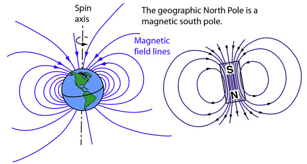
Fig. 1.16 The north pole of a compass needle is a magnetic north pole. It is attracted to the geographic North Pole, which is a magnetic south pole (opposite magnetic poles attract). Image Credit: Hyperphysics.

In situ magnetometers or radiation produced by accelerating charges (e.g., radio emissions) can be used as a respective direct or indirect detection of magnetic fields. The presence of localized aurorae is also indicative of a magnetic field. The magnetic field of a planet can be approximated by a dipole (bar magnet) with perturbations to account for their irregularities.

• All four giant planets, Earth, Mercury, and Jupiter’s moon Ganymede have magnetic fields generated in their interiors.

• Venus and comets have magnetic fields induced by their interaction with the solar wind.

• Mars and the Moon have localized crustal magnetic fields.

• Perturbations in Jupiter’s magnetic field near Europa and Callisto are indicative of salty oceans in their interiors.

• Geyser activity on Enceladus perturbs Saturn’s magnetic field.

1.4.8. Surface Composition

The composition of a body’s surface can be derived from:

• Spectral Reflectance Data: The absorption or emission spectra from a material gives clues to its composition. Various materials are heated on the surface and emit their radiation to be observed by orbiters (e.g., MAVEN). Such spectra may be observed from Earth, but certain wavelengths (e.g., UV) can only be observed from space.

• X-ray or \(\gamma\)-ray Fluorescence: Measurements conducted from a spacecraft (orbiter or flyby), where specific materials are emitting a short-wavelengths.

• Chemical Analysis of Surface Samples: Samples can be brought to Earth by natural process (i.e., meteorites) or spacecraft to be analyzed. In situ measurements can be performed although they usually provide less detail. Other forms of in situ analysis include mass spectroscopy, electrical conductivity, and thermal conductivity.

The compositions of the planets, asteroids, and satellites show a general dependence on heliocentric distance, where objects closer to the Sun have the largest concentrations of dense materials (i.e., refractory materials with a high melting and boiling temperature) and the smallest concentration of volatile materials (e.g., ices) that have a lower melting and boiling temperatures.

1.4.9. Surface Structure

The surface structure varies greatly between planets. There are various ways to determine a planet’s surface structure:

• Direct Imaging: Images taken either passively in the visible-radio wavelengths or actively using radar imaging techniques to detect large scale structures. It is best to have imaging available at multiple illumination angles to separate tilt-angle (slope) effects from albedo differences.

• Reflectivity Variations: Structure on small scales (e.g., grains) can be deduced from radar echo brightness and reflectivity variations with phase angle (i.e., the angle between the Sun and the observer as seen from the body). The brightness of a body with a size much larger than the wavelength of the observations generally increases slowly with decreasing phase angle. For very small phase angles, this increase can be much more rapid and is known as the opposition effect.

1.4.10. Atmosphere

Most of the major planets (and Titan) are surrounded by significant atmospheres. The giant planets are basically huge fluid balls, where their atmospheres are dominated by \(\rm H_2\) and \(He\). Venus and Mars are (currently) dominated by atmospheres primarily composed of \(\rm CO_2\), where the Venusian clouds are so thick that the surface is completely opaque for visible wavelengths. Earth’s atmosphere mainly consists of nitrogen \(\rm N_2\) (\(78\%\)) and oxygen \(\rm O_2\) \((21\%)\), where the remaining \(1\%\) is composed of a wide range of trace gases. The Martian atmosphere is in stark contrast to Venus, where its transparency has allowed for intense study for over a century.

Saturn’s satellite Titan has a dense nitrogen-rich atmosphere that intriguingly contains many kinds of organic molecules that are considered the building blocks of life (as we know it). Pluto and Neptune’s moon Triton each have a tenuous atmosphere dominated by \(N_2\). Jupiter’s volcanically active moon Io has a thin atmosphere composed of sulfur dioxide \(\rm SO_2\). Mercury and the Moon have an extremely tenuous atmosphere (\(\leq 10^{-12}\) bar). Mercury’s atmosphere contains atomic oxygen \(\rm O\), sodium \(\rm Na\), and helium \(\rm He\), where the Moon’s atmosphere is composed of argon \(\rm Ar\) and \(\rm He\).

The structure (i.e., temperature-pressure profile) and composition can be determined from

• spectral reflectance data at visible wavelengths,

• thermal spectra and photometry (in the IR and radio),

• stellar occultation profiles,

• in situ mass spectrometers, and

• attenuation of radio signals sent back to Earth by atmospheric/surface probes.

1.4.11. Interior

Planetary interiors are not directly accessible for observation, but one can derive information on a planet’s bulk composition and its interior structure. The bulk composition is deduce from a variety of direct and indirect constraints. The most fundamental are based on the mass and size of a planet. Jupiter and Saturn are composed primarily of hydrogen because all other elements are too dense to fit the constraints (e.g., size, mass, temperature, pressure) or known material properties that are derived from laboratory studies and quantum mechanical calculations.

Planets that are primarily composed of denser materials (than hydrogen) have compositions best estimated using models that include

• mass,

• radius,

• surface and atmospheric composition,

• heliocentric distance, and

• reasonable assumptions of cosmogonic abundances.

A planet’s internal structure can be derived (to some extent) from its gravitational field and rotation rate. From these parameters, the degree of mass concentration can be estimated. The gravitational field can be measured from spacecraft tracking or from the orbits of satellites/rings. Seismology provides more detailed information on the internal structure of a planet. The velocities and attenuation of seismic waves depend on the density, rigidity, composition, and temperature of the interior. Reflection and refraction off internal boundaries provide information on layering. The free oscillation periods of gaseous planets (e.g., kronoseismology) and stars (e.g., helioseismology) provides important information regarding the respective interiors.

The response of moons that are subject to significant time-dependent tidal deformations depends on their internal structure. Repeated observations can reveal the presence of a subsurface ocean. Measurements of the gravity field with altitude could show the extent of lateral inhomogeneities under the surface of icy moons and infer the presence of volcanic sources and tectonic structures that could melt the ice. Conducting fluid regions within a planetary interior are believed to be responsible for substantial magnetic fields. Centered dipole fields are probably produced in or near the core of the planet, whereas highly irregular offset fields are likely produced closer to the planet’s surface.

1.5. Formation of the Solar System

The nearly planar and low eccentricity orbits of the Solar System planets strongly support hypotheses for planet formation occurring from a flattened circumsolar disk. Astrophysical models suggest that disks are a natural by-product the star formation process resulting from the collapse of rotating molecular cloud cores. Molecular cloud cores are the coldest and densest parts of the interstellar medium. Observational evidence for analogs of a Solar System-like disks around young stars has increase substantially with observations from the Atacama Large Millimeter Array (ALMA). Infrared excesses in teh spectra of your stars suggest that protoplanetary disk lifetimes range from \(1-10\) million years (\(\rm Myr\)).

Numerous molecular clouds are found within our galaxy, where they are typically several orders of magnitude larger than our Solar System. Molecular clouds are inhomogeneous and are the sites in which star formation occurs. Even a very slowly rotating molecular cloud core has far too much spin angular momentum to collapse down to solar radius. A significant fraction of the material in a collapsing core falls onto a rotationally supported disk orbiting the pressure-supported protostar (see Fig. 1.17).

Fig. 1.17 This illustration shows the steps in the formation of the solar system from the solar nebula. As the nebula shrinks, its rotation causes it to flatten into a disk. Much of the material is concentrated in the hot center, which will ultimately become a star. Away from the center, solid particles can condense as the nebula cools, giving rise to planetesimals, the building blocks of the planets and moons. Image credit: OpenStax: Astronomy.

The disk has the same initial elemental composition as the growing star. At sufficient distances from the central star, it is cool enough for \(\sim1-2\%\) of the material to condense (i.e., cool) into either remnant interstellar grains or other solids. The dust is primarily composed of rock-forming compounds within a few AU of the host star, where solids in the outer regions grow along with ices (e.g., \(\rm H_2O\), \(\rm CH_4\), and \(\rm CO\)).

During the infall stage, the disk is very active and probably highly turbulent. Gravitational instabilities along with viscous and magnetic forces may add to the activity. When the infall slows substantially or stops, the disk becomes more quiescent (i.e., inactive). Interactions with the gaseous component of the disk affect the dynamics of small bodies, where they can grow from micron-sized (\(\mu \rm m\)) dust into kilometer-sized planetesimals. The details for this growth is still an active field of research today. Meteorites, minor planets, and comets best preserve a record of the important period in Solar System development.

The dynamics of larger solid bodies within protoplanetary disks are better characterized. The primary perturbations on these bodies are mutual gravitational interactions and physical collisions. Some interactions lead to collisions of planetesimals that are accretionary, where the incident bodies combine to form a larger object. However, some collisions actually lead to erosion (partial breakup) or complete fragmentation depending on the impact geometry or velocity. Eventually solid bodies grow into the terrestrial planets in the Solar System or into \(\sim 10\ M_\oplus\) planetary cores in the outer Solar System. The more massive cores are able to gravitationally attract and retain the leftover gas from the protoplanetary disk. In contrast, terrestrial planets accumulated only a small portion of the gas and were not massive enough to retain it against erosion from the solar wind. The gases (and water) in the current atmospheres of the terrestrial planets are derived from the planetary interior, which held material from the solid planetesimals.

The planets in our Solar System orbit close enough to one another that the final phases of planetary growth could have involved the merger or ejection of planets or planetary embryos on unstable orbits. Since the outer planets have such low eccentricities in their orbits, it appears that some damping process (e.g., accretion, ejection of numerous small planetesimals, or interactions with residual gas within the protoplanetary disk) must have been involved.

1.6. Homework

Problem 1

Because the distances between the planets are much larger than planetary sizes, very few diagrams or models of the Solar System are completely to scale. Imagine that you are preparing a demonstration for a 2nd grade class and you decide to use a 1-cm diameter marble to represent the Earth.

(a) What other objects can you use and how far apart must you space them?

(b) Proxima Centauri (the nearest star to the Solar System) is 4.2 light years away. In your model, where would you place it?

Problem 2

A planet that keeps the same hemisphere pointed towards the Sun must rotate once per orbit in the prograde direction.

(a) Draw a diagram to demonstrate this fact.

(b) The rotation rate of the Earth is one rotation (\(360^\circ\)) every 24 solar hours (i.e., length of the solar day). The rotation rate of the celestial sphere is one rotation every tropical year (365.2422 days). How many degrees must the Earth rotate per day on average over a year?

(c) A sidereal day is the time for a complete rotation relative to the background stars. Using your answer from (b), calculate the length of a sidereal day in decimal hours and \(hh\ mm\ ss\).

(d) Determine a general formula relating the lengths of the solar and sidereal days on a planet. Use your formula to compute the lengths of solar days on Mercury, Venus, Mars, and Jupiter.

Problem 3

The definition of a planet has become a semi-controversial topic, where some scientists believe Pluto’s planethood should be restored.

(a) What criteria defines a planet?

(b) If the conditions were loosened to make a Pluto a planet again, what would be the consequences?

(c) Is there a historical precedent for demoting celestial bodies? Does it make sense for Pluto?

Problem 4

Describe how an extrasolar observer might view our Solar System. What are the most conspicuous elements?

Problem 5

What are the most easily distinguished planetary properties within the Solar System? Describe how these features inform our search for extrasolar planets.