2. N-body Simulations

Solving orbital problems (even a two-body problem) can be a tricky business. Historically, the Kepler problem is difficult due to its transcendental nature. See Pál (2009) for an overview of solving the Kepler problem analytically. This section is dedicated to modern techniques of numerically solving the orbital problems, which contain an \(N\) number of bodies.

2.1. Available software

Here is a listing of some software packages available. Each package may have its particular advantages (e.g., low memory overhead, speed, GPU/CPU), but this section will mostly demonstrate usage of the Rebound package.

• Rebound

• Genga (GPU code)

• Mercury6; Mercury6_bin (binary star version)

• Swift

• HNbody

• Nbody6; Nbody6++GPU

• nbody

• Gadget2

• Galaxy

• Starlab

• AMUSE

2.2. A simple simulation (1 star + 2 planets)

Below is a guide to setting up a simple simulation using Rebound. Google Colab is a convenient tool to test out code in python, which is conveniently linked if you inspect the dropdown options on the rocketship at the top of this notebook.

Note

Google Colab is loaded with commonly used (basic) libraries and modules (e.g., matplotlib, numpy, and scipy). However to include external packages like Rebound, you will need to install it first. This is accomplished by running !pip install rebound in a code cell at the very beginning.

2.2.1. Structure of a (basic) Rebound simulation

A simulation in rebound consists of

1. importing the rebound library

2. creating a Simulation class instance,

3. defining the simulation parameters (e.g., integrator, timestep, units)

4. adding particles

5. adjusting the coordinate system

6. (optional) loading a simulation archive

7. running the simulation

A Simulation class instance allows you to reference functions and parameters linked to a given simulation. Consider a Simulation as the trunk of a tree, where functions and parameters are the branches. As a result, you can reference a given simulation parameter using the dot notation that is a part of python, C, and other programming languages. For example,

object = library.function()

illustrates how an instance of a function from a library can be initialized and stored into an object that can be referenced later.

A Simulation has some default parameters that are initialized unless you tell it otherwise. Here are some of those defaults:

• integrator is the IAS15 adaptive timestep algorithm,

• units defined using \(G=1\) (i.e., AU, Msun, \(\rm yr/2 \pi\)),

• timestep dt is \(0.001\ \rm [yr/2 \pi]\),

• exact_finish_time is set to \(1\), which means that the final timestep will be adjusted accordingly.

Below is an example simulation that creates an instance and sets up some of the simulation parameters. Our sample simulation will ultimately evaluate a 2 planet system consisting of Earth-mass planets orbiting a Sunlike star with orbital periods of \(9\) and \(15\) days. The simulation uses the whfast integrator, which is a more efficient method for some problems (see advanced whfast for more details). By default, the particles are added using Jacobi coordinates, where the move_to_com() function will convert to barycentric coordinates.

import rebound
import numpy as np

sim = rebound.Simulation()
sim.integrator = 'whfast' #using the WHfast algorithm 
sim.units = ('days', 'AU', 'Msun') #changed the time to days
sim.dt = 0.01 #steps of 0.01 days (unit inherited from above)

sim.add(m=1) #add a Sunlike star
sim.add(m=3e-5,P=9) #add planet with orbital period P = 9 days; circular orbit
sim.add(m=3e-5,P=15,f=np.pi) #add planet with orbital period P = 15 days; circular orbit
sim.move_to_com() #convert to barycentric

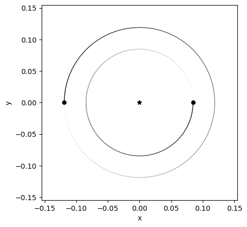
Rebound has some functions that interface with matplotlib (see matplotlib documentation for details), which is a library for creating high quality figures and plots. This method of visualization is useful to give you a idea of the system setup, or at a specific point in time. In the code below, it plots the host star (represented by a star) and each planet (dots). The \(x-y\) plane gives a top-down view of the system with units of AU along each axis.

%matplotlib inline
op = rebound.OrbitPlot(sim)

2.2.2. Saving a simulation

We can create a simulation archive to store samples of the system as it evolves. The automateSimulationArchive function allows us to specify a file name to store the samples, frequency for which to take samples (in time units given by sim.units), and whether to overwrite the previous file as a boolean.

Note

Replacing the interval argument with step is in general more reliable. The reason is that the number of timesteps is an integer value whereas the time is a floating point number. If you run long simulations, you might encounter issues with finite floating point precision. This only affects very high accuracy simulation where you want to make sure the outputs occur exactly at the right timestep.

sim.automateSimulationArchive("archive.bin",interval=0.45,deletefile=True) #9/20 = 0.45 days (or 20 samples per orbit of inner planet)
sim.integrate(9*1000) #integrate the orbits for 1000 periods of the inner planet; this takes a few (~3-4) minutes

The simulation archive stores each sample similar to a python list, where each object in the list is itself a simulation. Therefore, we can access the data file “archive.bin” iteratively by creating an instance of SimulationArchive (see SimulationArchive examples for details). We can then probe the simulation archive object sa using the dot convention for variables. Upon inspection, we find that the time of the first and last snapshots are 0 and 9000 days, respectively. The number of snapshots should be \(1+20/9 \cdot 9000\ \rm days = 20,001\ \rm days\) including the initial snapshot at \(t=0\).

sa = rebound.SimulationArchive("archive.bin")
print("Number of snapshots: %d" % len(sa))
print("Time of first and last snapshot: %.1f, %.1f" % (sa.tmin, sa.tmax))

Number of snapshots: 20001
Time of first and last snapshot: 0.0, 9000.0

/home/saturnaxis/anaconda3/lib/python3.9/site-packages/rebound/simulationarchive.py:99: RuntimeWarning: Binary file was saved with a different version of REBOUND. Binary format might have changed.
  warnings.warn(message, RuntimeWarning)

2.2.3. Plotting a simulation

To plot a simulation, we can use samples from the SimulationArchive and create a visualization through matplotlib. The example below walks through the basic setup of creating a plot, where there are many ways to customize the appearance (see matplotlib documentation for more details).

First, we need to access the functions within the matplotlib library and more specificially, those in the pyplot sublibrary. In python, this is done through the import statement and we can denote a reference label plt,

import matplotlib.pyplot as plt

so that we can more easily reference the functions without using the full path to the function.

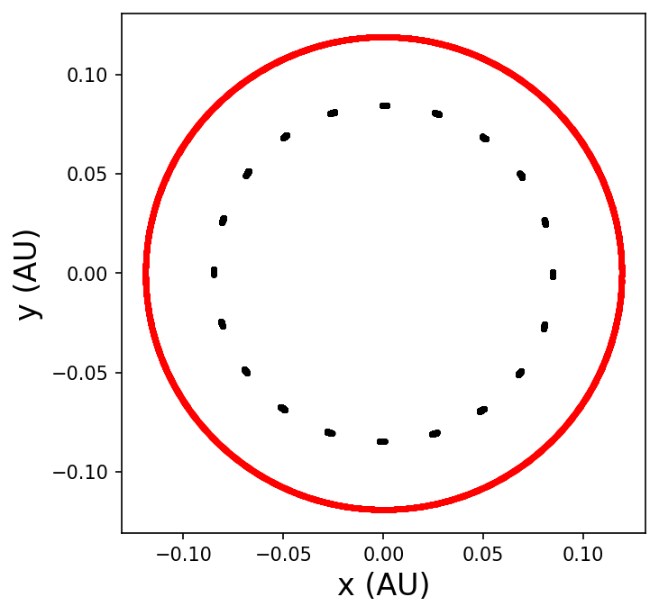
The simulation above considers two planets, where we can designate data points for each planet by color: inner (black) and outer (red). Also we know that there will be three particles (star, inner planet, outer planet) and the ps list holds objects representing each body at each snapshot in time. Therefore, it would be convenient to iterate through the colors following the same counting scheme as we iterate through the particles (i.e., particle index \(i = \{0,\ 1,\ 2\}\)). Let’s define a color list as

color = ['','k','r']

where this list skips the position zero (using an empty string '') for the host star, assigns 'k' (black) in the first position, and 'r' (red) in the final position. A for loop that iterates through the particles will begin at \(0\) and continue non-inclusively until it reaches \(3\) (i.e., only evaluating \(i = \{0,\ 1,\ 2\}\)).

Then, a figure instance is created using the plt label. Arguments of the figure can include the:

• size of the figure; figsize=(w,h) with the width w and height h measured in inches,

• resolution of the figure in dots per inch dpi; the default is \(75\), but it is often better to use \(150\).

Following the figure is the creation of a reference axis ax by using the function add_subplot. This function creates a canvas for which to add our points and requires information concerning the number of rows \(r\), columns \(c\), and the index \(i\) of the subplot. Together these instances are

fig = plt.figure(figsize=(5,5),dpi=150)
ax = fig.add_subplot(111)

where h=w=5, dpi=150, and rci=111.

The simulation archive is sampled using a for loop that iterates through each snapshot, while a second for loop iterates through the particles. Within the second for loop dots are plotted onto the axis ax with a marker '.' (dot) and markersize ms=4. Note that we expect ~20 equally spaced positions for the inner planet (due to our output sampling) and a continuous curve for the outer planet. In python, this code is:

for s in range(0,len(sa)):
    sim = sa[s] #iterate through each snapshot in sa
    ps = sim.particles #intermediate object to simpify the referencing
    for i in range(1,len(ps)): #iterate through each of the particles, skipping the host star 
        ax.plot(ps[i].x,ps[i].y,'.',ms=4,color=color[i])

To make the resulting plot easier to read later, we can add labels to the \(x\)- and \(y\)-axis as strings and denote the point size of the font in fontsize. The final line should contain a semicolon ; at the end to prevent extra output. The code for this customization is given by:

ax.set_xlabel("x (AU)",fontsize=16)
ax.set_ylabel("y (AU)",fontsize=16);

Altogether, we can combine these statements into one code as:

import matplotlib.pyplot as plt

color = ['','k','r']

fig = plt.figure(figsize=(5,5),dpi=150)
ax = fig.add_subplot(111)

for s in range(0,len(sa)):
    sim = sa[s] #iterate through each snapshot in sa
    ps = sim.particles #intermediate object to simpify the referencing
    for i in range(1,len(ps)): #iterate through each of the particles, skipping the host star 
        ax.plot(ps[i].x,ps[i].y,'.',ms=4,color=color[i])
ax.set_xlabel("x (AU)",fontsize=16)
ax.set_ylabel("y (AU)",fontsize=16);

/home/saturnaxis/anaconda3/lib/python3.9/site-packages/rebound/simulationarchive.py:146: RuntimeWarning: Binary file was saved with a different version of REBOUND. Binary format might have changed.
  warnings.warn(message, RuntimeWarning)

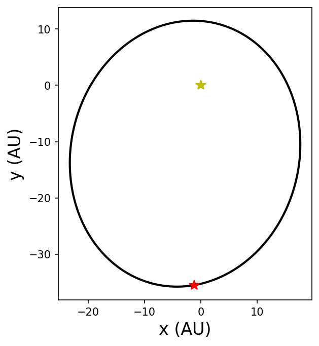
2.3. Simulating \(\alpha\) Cen AB

To simulate the orbit of \(\alpha\) Cen AB, we need to use the known orbital parameters. The stellar masses and orbital elements are given in Introduction to the \(\alpha\) Centauri System, but we’ll use the binary orbital plane as a reference so that \(i = \Omega = 0^\circ\) and \(\omega = 77.05^\circ = (232.3^\circ + 204.75^\circ) \mod 360^\circ\). Additionally, we need to specifiy a starting position using true anomaly \(f\) or mean anomaly MA. Quarles & Lissauer (2016) calculated the binary mean anomaly for Julian date (JD) 2452276, which is \(209.6901^\circ\) and we’ll use it here (Quarles & Lissauer 2016).

import rebound 
import numpy as np
import matplotlib.pyplot as plt

M_A = 1.133 #mass of star A in solar masses
M_B = 0.972 #mass of star B in solar masses
a_bin = 23.78 #semimajor axis in AU
e_bin = 0.524 #eccentricity
omg_bin = np.radians(77.05) #pericenter of binary converted to radians
MA_bin = np.radians(209.6901) #mean anomaly of binary @ JD 2452276
T_bin = np.sqrt(a_bin**3/(M_A+M_B)) #period of the binary in years

sim = rebound.Simulation()
sim.integrator = 'whfast'
sim.units = ('yr','Msun','AU')
sim.dt = 0.01 

sim.add(m=M_A)
sim.add(m=M_B,a=a_bin,e=e_bin,omega=omg_bin,M=MA_bin) #i=Omega=0 by default
sim.move_to_com()  #convert to center of mass coordinates

sim.automateSimulationArchive("alphaCen.bin",interval=0.1,deletefile=True)
sim.integrate(T_bin)

#plot the simulation
sa = rebound.SimulationArchive("alphaCen.bin")

fig = plt.figure(figsize=(5,5),dpi=150)
ax = fig.add_subplot(111)
ax.set_aspect('equal')

ax.plot(0,0,'y*',ms=10)
xy_bin = np.zeros((len(sa),2))
for s in range(0,len(sa)):
    sim = sa[s] #iterate through each snapshot in sa
    ps = sim.particles #intermediate object to simpify the referencing
    sim.move_to_hel() #shift to astrocentric coordinates
    xy_bin[s,:] = [ps[1].x,ps[1].y]
ax.plot(xy_bin[:,0],xy_bin[:,1],'k-',lw=2)
ax.plot(xy_bin[0,0],xy_bin[0,1],'r*',ms=10)
ax.set_xlabel("x (AU)",fontsize=16)
ax.set_ylabel("y (AU)",fontsize=16);

2.4. Adding a planet

In \(\alpha\) Cen AB, we can add a planet orbiting either star (S-Type) or both stars (P-Type). In rebound particles are added in the order given in your python code and using Jacobi coordinates by default. As a result there can be some ambiguity between a planet orbiting star B (S-Type) and a circumbinary planet orbiting both stars (P-Type). To resolve this, the following convention forces the planet into S-Type:

sim.add(m=M_host) #add the host star mass (could be either A or B)
sim.add(m=m_pl, a=a_pl, e=e_pl, ...) #add the planet using either orbital elements or Cartesian coordinates relative to the host star
sim.add(m=M_sec, a=a_bin, e=e_bin, ...) #add the secondary star relative to the host star (i.e., like a big planet)
sim.move_to_com()

where the adding the secondary star first forces the planet into P-Type:

sim.add(m=M_host) #add the host star mass (could be either A or B)
sim.add(m=M_sec, a=a_bin, e=e_bin, ...) #add the secondary star relative to the host star
sim.add(m=m_pl, a=a_pl, e=e_pl, ...) #add the planet using either orbital elements or Cartesian coordinates relative to the center of mass
sim.move_to_com()

Note

There is a argument in the add function called primary, which redirects the action to add the particle relative to the primary object (see here for more details). This could be an option to add S-Type planets orbiting both stars, where a change in reference would not work.

2.4.1. Example simulation

As an example, let’s add an Earth-like planet on a circular, coplanar orbit around \(\alpha\) Cen A with a semimajor axis \(a_{\rm pl} = 1\ \rm AU\). In the code below: we add

• some global variables for the planet,

• the particle in an appropriate order, and

• update the indices for plotting (i.e., 0 = star A, 1 = planet, 2 = star B).

import rebound 
import numpy as np
import matplotlib.pyplot as plt

M_A = 1.133 #mass of star A in solar masses
M_B = 0.972 #mass of star B in solar masses
a_bin = 23.78 #semimajor axis in AU
e_bin = 0.524 #eccentricity
omg_bin = np.radians(77.05) #pericenter of binary converted to radians
MA_bin = np.radians(209.6901) #mean anomaly of binary @ JD 2452276
T_bin = np.sqrt(a_bin**3/(M_A+M_B)) #period of the binary in years

M_pl = 3.0035e-6 #mass of Earth in solar masses
a_pl = 1. #semimajor axis in AU

sim = rebound.Simulation()
sim.integrator = 'whfast'
sim.units = ('yr','Msun','AU')
sim.dt = 0.01 

sim.add(m=M_A)
sim.add(m=M_pl,a=a_pl)
sim.add(m=M_B,a=a_bin,e=e_bin,omega=omg_bin,M=MA_bin) #i=Omega=0 by default
sim.move_to_com()  #convert to center of mass coordinates

sim.automateSimulationArchive("alphaCen_wPl.bin",interval=0.1,deletefile=True)
sim.integrate(T_bin)

#plot the simulation
sa = rebound.SimulationArchive("alphaCen_wPl.bin")

fig = plt.figure(figsize=(5,5),dpi=150)
ax = fig.add_subplot(111)
ax.set_aspect('equal')

ax.plot(0,0,'y*',ms=10)
xy_bin = np.zeros((len(sa),2))
xy_pl = np.zeros((len(sa),2))
for s in range(0,len(sa)):
    sim = sa[s] #iterate through each snapshot in sa
    ps = sim.particles #intermediate object to simplify the referencing
    sim.move_to_hel() #shift to astrocentric coordinates
    xy_bin[s,:] = [ps[2].x,ps[2].y]
    xy_pl[s,:] = [ps[1].x,ps[1].y]
ax.plot(xy_bin[:,0],xy_bin[:,1],'k-',lw=2)
ax.plot(xy_bin[0,0],xy_bin[0,1],'r*',ms=10)
ax.plot(xy_pl[:,0],xy_pl[:,1],'k-',lw=2)
ax.plot(xy_pl[0,0],xy_pl[0,1],'b.',ms=10)

ax.set_xlabel("x (AU)",fontsize=16)
ax.set_ylabel("y (AU)",fontsize=16);

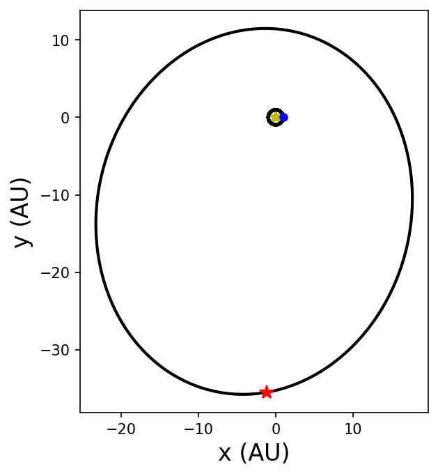
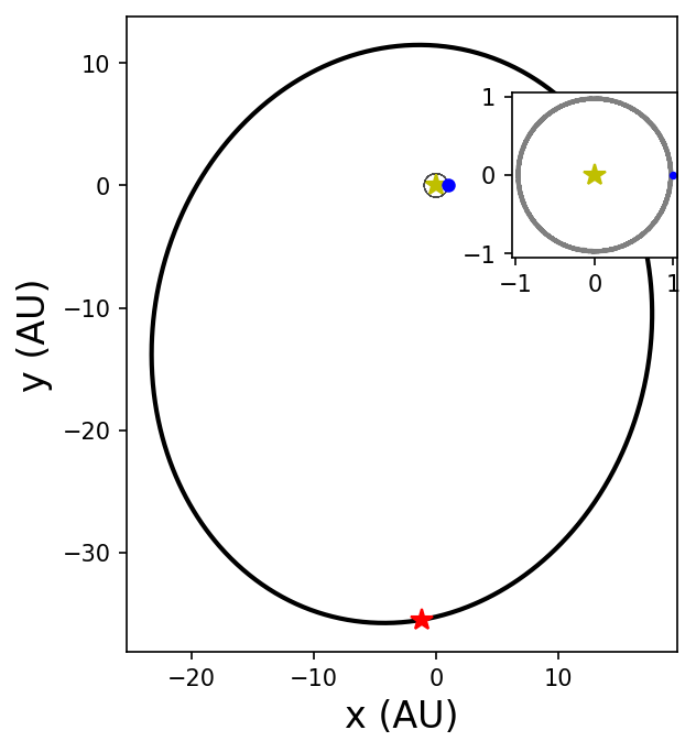
Due to the difference in scale between the planetary and binary orbits, it is difficult to visualize both at the same time. The matplotlib library has an important function called inset_axes that generates a separate (child) axis relative to a different (parent) axis. This allows us to zoom in on the planetary orbit within the inset. The code below demonstrates the necessary modifications for an inset.

from mpl_toolkits.axes_grid1.inset_locator import inset_axes

#plot the simulation
sa = rebound.SimulationArchive("alphaCen_wPl.bin")

fig = plt.figure(figsize=(5,5),dpi=150)
ax = fig.add_subplot(111)
axins = inset_axes(ax, width="100%", height="50%", bbox_to_anchor=(.7, .5, .3, .5), bbox_transform=ax.transAxes)
ax.set_aspect('equal')
axins.set_aspect('equal')

ax.plot(0,0,'y*',ms=10)
axins.plot(0,0,'y*',ms=10)
xy_bin = np.zeros((len(sa),2))
xy_pl = np.zeros((len(sa),2))
for s in range(0,len(sa)):
    sim = sa[s] #iterate through each snapshot in sa
    ps = sim.particles #intermediate object to simplify the referencing
    sim.move_to_hel() #shift to astrocentric coordinates
    xy_bin[s,:] = [ps[2].x,ps[2].y]
    xy_pl[s,:] = [ps[1].x,ps[1].y]
ax.plot(xy_bin[:,0],xy_bin[:,1],'k-',lw=2)
ax.plot(xy_bin[0,0],xy_bin[0,1],'r*',ms=10)
ax.plot(xy_pl[:,0],xy_pl[:,1],'k-',lw=0.1,alpha=0.7)
ax.plot(xy_pl[0,0],xy_pl[0,1],'b.',ms=10)

axins.plot(xy_pl[:,0],xy_pl[:,1],'k-',lw=0.1,alpha=0.5)
axins.plot(xy_pl[0,0],xy_pl[0,1],'b.',ms=5)
axins.set_xlim(-1.05,1.05)
axins.set_ylim(-1.05,1.05)

ax.set_xlabel("x (AU)",fontsize=16)
ax.set_ylabel("y (AU)",fontsize=16);

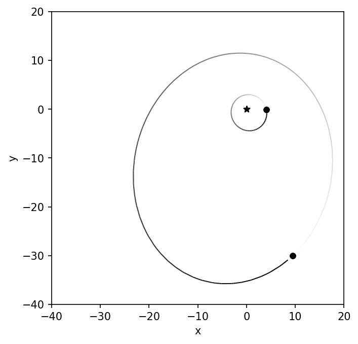
2.4.2. Animating a simulation

The above example produces a stack of snapshots to visually represent the simulation. In some cases, it can be more visually stimulating and illuminating if the data visualization is animated. An animation is essentially a stack of images that are viewed in succession with a short delay. To create the animation, we must first create a stack of images. Within the API of rebound, there are some functions that can make this process easier. Note that using rebound in this manner is not the only way.

import rebound
import numpy as np
import os

home = os.getcwd() + "/Tutorials/"

M_A = 1.133 #mass of star A in solar masses
M_B = 0.972 #mass of star B in solar masses
a_bin = 23.78 #semimajor axis in AU
e_bin = 0.524 #eccentricity
omg_bin = np.radians(77.05) #pericenter of binary converted to radians
MA_bin = np.radians(209.6901) #mean anomaly of binary @ JD 2452276
T_bin = np.sqrt(a_bin**3/(M_A+M_B)) #period of the binary in years

M_pl = 3.0035e-6 #mass of Earth in solar masses
a_pl = 4. #semimajor axis in AU

sim = rebound.Simulation()
sim.integrator = 'ias15'
sim.units = ('yr','Msun','AU')
sim.dt = 0.001

sim.add(m=M_A)
sim.add(m=M_pl,a=a_pl,primary=sim.particles[0])
sim.add(m=M_B,a=a_bin,e=e_bin,omega=omg_bin,M=MA_bin) #i=Omega=0 by default
sim.move_to_com()  #convert to center of mass coordinates

#Rebound plotting
#https://github.com/hannorein/rebound/blob/a668eaebb691f3cf54f4f3698db0f6f34ea7aa2c/rebound/plotting.py#L7
op = rebound.OrbitPlot(sim)

fig = op.fig
op.update()
op.ax.set_xlim(-40,20)
op.ax.set_ylim(-40,20)
op.fig.set_size_inches(5, 5)
op.fig.set_dpi(150)

if not os.path.exists(home+"Plots/"):
    os.makedirs(home+"Plots/")
else:
    pnglist = [f for f in os.listdir(home+"Plots/") if f.endswith('png')]
    for png in pnglist:
        os.remove(home+"Plots/" + png)

for i in range(0,250):
    op.sim.integrate(sim.t+1)
    sim.move_to_hel()
    op.update()       # update data
    fig.canvas.draw() # redraw figure
    op.fig.savefig(home+"Plots/out_%03d.png" % i, bbox_inches='tight',dpi=150)
    sim.move_to_com();

After creating the stack of images, we can use imagemagick to convert it into an animated gif using convert. The subprograms from imagemagick are not installed by default within Google Colab. To install it, simply create a python cell with the following !apt install imagemagick to install imagemagick from an open source linux repository.

The convert program uses a series of command line arguments, which tell the program how to format the output and where the input is located. In the above code we created a subdirectory called Plots, and thus we need to change to that directory. Some command line arguments to define are delay, loop, dispose, the png stack, and the absolute path of the animated gif file.

%cd /content/Plots/
!convert -delay 10 -loop 0 -dispose previous *.png /content/animation_example.gif

Alternatively, the convert can be used from the terminal, if you already have imagemagick installed locally. Then you can either call it from the terminal or from python using the subprocess module.

import subprocess as sb 
os.chdir(home+"Plots/")
sb.run("convert -delay 10 -loop 0 -dispose previous *.png %sanimation_example.gif" % home,shell=True);

The result is an animated gif that represents the simulation. From the animation, we can see that the planetary eccentricity and argument of pericenter are modified after every binary periastron passage. The perturbation that changes the argument of pericenter does not preferentially rotate in either direction: clockwise or counter-clockwise. At least not on the timescale of a few binary orbits.

Fig. 2.1 Example animation created using a stack of png images and imagemagick.

2.5. References

• Quarles & Lissauer (2016)