1. Introduction to the α Centauri System#
1.1. The stellar parameters#
The \(\alpha\) Centauri system is a collection of three stars that are \({\sim}4\ \rm ly\) away from our Sun. Two of the stars are Sunlike (\(\alpha\) Cen AB), which means that they share a similar mass or luminosity to our Sun. The third star (Proxima Centauri) is much cooler and smaller than our Sun. The physical parameters (i.e., mass, luminosity, and radius in solar units) for \(\alpha\) Cen AB from Pourbaix & Boffin (2016) (\(\alpha\) Cen AB) are given in the table below:
parameters |
\(\alpha\) Cen A |
\(\alpha\) Cen B |
|---|---|---|
mass \((M_\odot)\) |
\(1.105 \pm 0.0070\) |
\(0.934 \pm 0.0061\) |
luminosity \((L_\odot)\) |
\(1.519 \pm 0.018\) |
\(0.5002 \pm 0.016\) |
radius \((R_\odot)\) |
\(1.231 \pm 0.0036\) |
\(0.868 \pm 0.0052\) |
Note
The mass and radius used here are from Pourbaix & Boffin (2016), while the luminosity used is from Thévenin et al. (2002). These values have been updated recently by Akeson et al. (2021), but the older values are retained for consistency with prior works.
Proxima Centauri is ignored in this JupyterBook because it is significantly less massive and has a close approach (periastron passage) of \({\gtrsim} 3,500\ \rm AU\) (Akeson et al. (2021)), which implies that it likely has a negligible gravitational effect on the inner binary and any extant planets orbiting either star.
These stars can be observed in the skies of the the southern hemisphere, where \(\alpha\) Cen AB appears as a single star to the naked eye. \(\beta\) Centauri is some \(4.5^\circ\) to the west on the sky and Proxima Centauri lies about \(2.2^\circ\) to the southwest of \(\alpha\) Cen AB. Recall that the angular diameter of the full Moon is \({\sim}0.5^\circ\), which means that Proxima lies \({\sim}4\) times the angular width of the Moon from \(\alpha\) Cen AB on the sky.

Fig. 1.1 The two bright stars are (left) Alpha Centauri and (right) Beta Centauri, both binaries. The faint red star in the center of the red circle, to the lower left from the center point between Alpha and Beta, and southwest of Alpha, is Proxima Centauri, intensely red, smaller in size, weaker in brightness and a distant third element in a triple star system with the main close pair forming Alpha Centauri. Figure credit: Wikipedia:Alpha_Centauri; user:Skatebiker.#
The \(\alpha\) Cen AB system has been subject to many observation campaigns in the search for nearby exoplanets. This has led to a few false positives (i.e., claimed detections that turned out spurious). In contrast to most stars, \(\alpha\) Cen AB is too bright with an apparent magnitude of \(V=0.01\) (\(\alpha\) Cen A) and \(V=+1.33\) (\(\alpha\) Cen B). Modern observational techniques use charge-coupled devices (CCDs) to record the light coming from a star through the telescope. \(\alpha\) Cen AB tends to saturate (overexpose) the CCD, which it makes it very difficult to measure fluctuations in the light.
Zhao et al. (2018) demonstrated that any planets orbiting \(\alpha\) Cen AB must be \(\lesssim 50\ M_\odot\), where \(1\ M_\oplus\) corresponds to the mass of the Earth, because otherwise such planets would have been detected after decades of observation. This may acutally be a good thing, if we are searching for Earthlike exoplanets.
1.2. The binary orbit#
There are two ways to measure the motion of two orbiting bodies in space: astrometry and radial velocity. Through astrometry, we measure the transverse motion that occurs perpendicular to our line of sight. For example, if I draw a circle on a whiteboard, the movement of the marker tip moves perpendicular to your line of sight (assuming that the whiteboard is mounted on a wall). Measurements using the radial velocity only capture the movement along your line of sight (i.e., in or out of the board).
Clearly, neither of these techniques provides the whole picture. Thus, it is common to use a combination of astrometry and radial velocity to determine the full orbit.
1.2.1. What is an orbit?#
A bound orbit is defined by an ellipse using Kepler’s laws. To draw an ellipse in a plane, we require 3 quantities:
semimajor axis \(a\),
eccentricity \(e\), and
argument of pericenter \(\omega\).
The semimajor axis defines the size of the orbit (i.e., how big it is), where the eccentricity modifies the shape of the orbit (i.e., how squashed it is). Together, these two quantities can make an ellipse. However, the argument of pericenter determines how much the pericenter rotates relative to a reference axis. Typically, we use the reference axis to be our line of sight.
The distance \(r\) from star A to any point on an orbit is defined as
where the true anomaly \(f\) measures the position along the orbit (relative to the argument of pericenter). Two points are defined along the semimajor axis that denote the closest (pericenter, \(q\)) and farthest (apocenter, \(Q\)) point from the reference star (see Fig. 1.2). Mathematically, these are given as
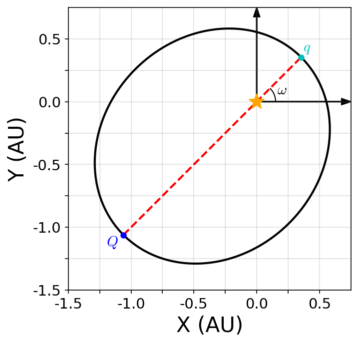
Fig. 1.2 Elliptical orbit \((e=0.5)\) with the reference star (orange star) at one focus. The major axis (red dashed line) connects the apocenter (blue dot) to the pericenter, where the semimajor axis \(a=1\ \rm AU\). The orbit is tilted relative to the reference axis (\(x\)-axis) by \(\omega = 45^\circ\).#
Show code cell content
import numpy as np
import matplotlib.pyplot as plt
from matplotlib import rcParams
from myst_nb import glue

rcParams.update({'font.size': 14})
rcParams.update({'mathtext.fontset': 'cm'})

#Assume the following:
semi = 1. # semimajor axis (in AU)
ecc = 0.5 #eccentricity
omg = np.radians(45) #argument of pericenter (converted to radians)

fs = 'x-large'

def ellipse(a,e,omega):
    #function to define an ellipse
    #semimajor axis a (in AU), eccentricity e (unitless)
    #argument of pericenter omega (radians)
    f_step = 0.01
    f = np.arange(0,2*np.pi+f_step,f_step)
    r = a*(1-e**2)/(1.+e*np.cos(f))
    return np.array([r*np.cos(omega+f),r*np.sin(omega+f)]) #return x,y coordinates of ellipse

fig = plt.figure(figsize=(5,5),dpi=150)
ax = fig.add_subplot(111)

ax.grid(True,color='gray',alpha=0.25)
ax.set_aspect('equal')

ax.arrow(0,0,0.75,0,width=0.005,head_width=0.05,color='k',length_includes_head=True)
ax.arrow(0,0,0,0.75,width=0.005,head_width=0.05,color='k',length_includes_head=True)

ell = ellipse(semi,ecc,omg)
peri, apo = semi*(1-ecc), semi*(1+ecc)
ax.plot(ell[0,:],ell[1,:],'k-',lw=2)
ax.plot([apo*np.cos(omg+np.pi),peri*np.cos(omg)],[apo*np.sin(omg+np.pi),peri*np.sin(omg)],'r--',lw=2)
ax.plot(apo*np.cos(omg+np.pi),apo*np.sin(omg+np.pi),'b.',ms=10)
ax.plot(peri*np.cos(omg),peri*np.sin(omg),'c.',ms=10)

arc_r = 0.15
ang_rng = np.radians(np.arange(0,45,1))
arc_x, arc_y = arc_r*np.cos(ang_rng), arc_r*np.sin(ang_rng)
ax.plot(arc_x,arc_y,'k-',lw=1)
ax.text(0.2,0.06,'$\omega$',horizontalalignment='center',rotation=0,fontsize='medium')
ax.text(0.4,0.4,'$q$',horizontalalignment='center',rotation=0,fontsize='medium',color='c')
ax.text(-1.15,-1.15,'$Q$',horizontalalignment='center',rotation=0,fontsize='medium',color='b')

ax.plot(0,0,'*',color='orange',ms=15)

ax.set_xlabel("X (AU)",fontsize = fs)
ax.set_ylabel("Y (AU)",fontsize = fs)
ax.set_xlim(-1.5,0.75)
ax.set_ylim(-1.5,0.75)
ticks = np.arange(-1.5,0.75,0.25)
ax.set_xticks(ticks)
ax.set_yticks(ticks)
xlabels, ylabels = [], []
for i in range(0,len(ticks)):
    if i % 2:
        xlabels.append("")
        ylabels.append("")
    else:
        xlabels.append(str(ticks[i]))
        ylabels.append(str(ticks[i]))
ax.set_xticklabels(xlabels)
ax.set_yticklabels(xlabels)

glue("orbit_fig", fig, display=False);
Thus far, we’ve used 3 parameters to draw an ellipse that is perpendicular to our line of sight. Note that a single point on the ellipse can be located using the true anomaly \(f\). However, the universe does not always provide “face-on” systems that are perpendicular to our line of sight. But we can transform our picture to the one provided by the universe using the appropriate rotation matrix. Notice that the rotation by the argument of pericenter used the rotation about the \(z\)-axis. The rotation matrices are:
where \(\theta\) represents a given rotation angle and following a right-hand rule. To rotate the argument of pericenter, we performed the following transformation: \(\vec{x}^\prime = R_z(\omega)\vec{x}\), where \(\vec{x} = \{r\cos{f},\ r\sin{f},\ 0\}\). We rotated a vector (that initially pointed along the \(x\)-axis) counter-clockwise because our right hand curls that way if your thumb points in the \(+z\).
A rotation about the \(x\)-axis moves positive \(y\) side of the ellipse towards our line of sight, while the negative \(y\) side moves away (i.e., in the radial direction). A transiting system would show a transverse motion along the \(x\)-axis, and a radial motion along the \(z\)-axis. To get there, we need to apply the \(R_x\) matrix using the rotation angle \(i\), which is called inclination. When \(i=90^\circ\), then the motion is along our line of sight.
The inclination (on the sky) for \(\alpha\) Cen AB is \({\sim}79^\circ\), we’ll use this as an example of a non-face-on orbit. Figure 1.3 illustrates how our view of an ellipse changes with respect to the inclination relative to the sky.
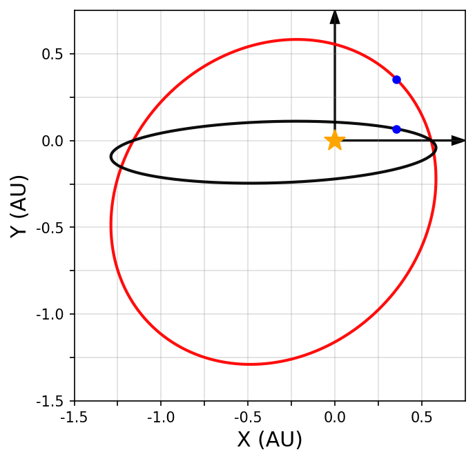
Fig. 1.3 Elliptical orbit from Fig. 1.2 (red), but rotated with an inclination \(i=79^\circ\) (black). The blue dots show the point transformation from one ellipse to the other.#
Show code cell content
import numpy as np
import matplotlib.pyplot as plt
from matplotlib import rcParams
from myst_nb import glue

rcParams.update({'font.size': 14})
rcParams.update({'mathtext.fontset': 'cm'})

def Rotate_x(x,theta):
    R_x = np.array([[1,0,0],[0,np.cos(theta),-np.sin(theta)],[0,np.sin(theta),np.cos(theta)]])
    return np.dot(R_x,x)
def Rotate_y(x,theta):
    R_y = np.array([[np.cos(theta),0,np.sin(theta)],[0,1,0],[-np.sin(theta),0,np.cos(theta)]])
    return np.dot(R_y,x)
def Rotate_z(x,theta):
    R_z = np.array([[np.cos(theta),-np.sin(theta),0],[np.sin(theta),np.cos(theta),0],[0,0,1]])
    return np.dot(R_z,x)

def get_ellipse(rvec,omega,true_f,inc):
    #get points of an ellipse given radii (array), omega (constant), true anomaly f (array) and inclination (constant)
    ellipse = np.zeros((len(rvec),3))
    for i in range(0,len(rvec)):
        x  =  rvec[i,:]
        xp = Rotate_z(x,omega)
        ellipse[i,:] = Rotate_x(xp,inc)
    return ellipse

#Assume the following:
semi = 1. # semimajor axis (in AU)
ecc = 0.5 #eccentricity
omg = np.radians(45) #argument of pericenter (converted to radians)
incl = np.radians(79) #inclination on the sky (converted to radians)

fs = 'x-large'

f_step = 0.01
f = np.arange(0,2*np.pi+f_step,f_step)
r = semi*(1-ecc**2)/(1.+ecc*np.cos(f))
r_vec = np.zeros((len(r),3))
r_vec[:,0], r_vec[:,1] = r*np.cos(f), r*np.sin(f)

fig = plt.figure(figsize=(5,5),dpi=150)
ax = fig.add_subplot(111)

ax.grid(True,color='gray',alpha=0.25)
ax.set_aspect('equal')

ax.arrow(0,0,0.75,0,width=0.005,head_width=0.05,color='k',length_includes_head=True)
ax.arrow(0,0,0,0.75,width=0.005,head_width=0.05,color='k',length_includes_head=True)

ell = get_ellipse(r_vec,omg,f,0)
ax.plot(ell[:,0],ell[:,1],'-',color='r',alpha=0.95,lw=2)
ax.plot(ell[0,0],ell[0,1],'b.',ms=10)

ell = get_ellipse(r_vec,omg,f,incl)
ax.plot(ell[:,0],ell[:,1],'-',color='k',alpha=0.95,lw=2)
ax.plot(ell[0,0],ell[0,1],'b.',ms=10)

ax.plot(0,0,'*',color='orange',ms=15)

ax.set_xlabel("X (AU)",fontsize = fs)
ax.set_ylabel("Y (AU)",fontsize = fs)
ax.set_xlim(-1.5,0.75)
ax.set_ylim(-1.5,0.75)
ticks = np.arange(-1.5,0.75,0.25)
ax.set_xticks(ticks)
ax.set_yticks(ticks)
xlabels, ylabels = [], []
for i in range(0,len(ticks)):
    if i % 2:
        xlabels.append("")
        ylabels.append("")
    else:
        xlabels.append(str(ticks[i]))
        ylabels.append(str(ticks[i]))
ax.set_xticklabels(xlabels)
ax.set_yticklabels(xlabels)


glue("rotate_fig", fig, display=False);
The argument of pericenter \(\omega\) rotates the orbit around the \(z\)-axis, where Fig. 1.3 has two points (or nodes) that cross the \(x\)-axis. If we define a reference plane where \(z=0\), then the orbiting body appears to ascend (move from \(-z\) to \(+z\)) at one node and descend (move from \(+z\) to \(-z\)) as it moves through the node. The longitude of ascending node \(\Omega\) defines the former, where the latter is called the descending node. The ascending node is defined from \(0^\circ-359^\circ\) and wraps around (e.g., \(359^\circ + 1^\circ \rightarrow 0^\circ\)).
There is not particular reason the orbit should align with our reference direction (the \(x\)-axis). Therefore, the ascending node rotates the orbit about the \(z\)-axis similarly to the rotation from the argument of pericenter (i.e., \(R_z(\Omega)\)).
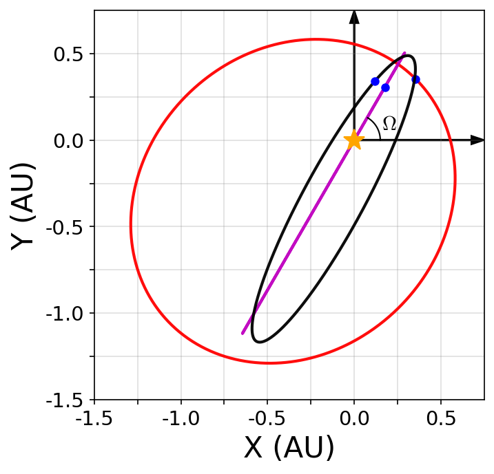
Fig. 1.4 Elliptical orbit from Fig. 1.2 (red), but rotated with an inclination \(i=79^\circ\) (black) or \(i=90^\circ\) (magenta). The inclined orbits (black and magenta) are also rotated with \(\Omega = 60\), to illustrate the changing of the ascending node. The blue dots show the point transformation from one ellipse to the other.#
Show code cell content
import numpy as np
import matplotlib.pyplot as plt
from matplotlib import rcParams
from myst_nb import glue

rcParams.update({'font.size': 14})
rcParams.update({'mathtext.fontset': 'cm'})

def Rotate_x(x,theta):
    R_x = np.array([[1,0,0],[0,np.cos(theta),-np.sin(theta)],[0,np.sin(theta),np.cos(theta)]])
    return np.dot(R_x,x)
def Rotate_y(x,theta):
    R_y = np.array([[np.cos(theta),0,np.sin(theta)],[0,1,0],[-np.sin(theta),0,np.cos(theta)]])
    return np.dot(R_y,x)
def Rotate_z(x,theta):
    R_z = np.array([[np.cos(theta),-np.sin(theta),0],[np.sin(theta),np.cos(theta),0],[0,0,1]])
    return np.dot(R_z,x)

def get_ellipse(rvec,omega,true_f,inc,RA):
    #get points of an ellipse given rvec (array), omega (constant), true anomaly f (array) and inclination (constant)
    ellipse = np.zeros((len(rvec),3))
    for i in range(0,len(rvec)):
        xp = Rotate_z(rvec[i,:],omega)
        xp = Rotate_x(xp,inc)
        ellipse[i,:] = Rotate_z(xp,RA)
    return ellipse

#Assume the following:
semi = 1. # semimajor axis (in AU)
ecc = 0.5 #eccentricity
omg = np.radians(45) #argument of pericenter (converted to radians)
incl = np.radians(79) #inclination on the sky (converted to radians)
RA_omg = np.radians(60) #longitude of ascending node

fs = 'x-large'

f_step = 0.01
f = np.arange(0,2*np.pi+f_step,f_step)
r = semi*(1-ecc**2)/(1.+ecc*np.cos(f))
r_vec = np.zeros((len(r),3))
r_vec[:,0], r_vec[:,1] = r*np.cos(f), r*np.sin(f)

fig = plt.figure(figsize=(5,5),dpi=150)
ax = fig.add_subplot(111)

ax.grid(True,color='gray',alpha=0.25)
ax.set_aspect('equal')

ax.arrow(0,0,0.75,0,width=0.005,head_width=0.05,color='k',length_includes_head=True)
ax.arrow(0,0,0,0.75,width=0.005,head_width=0.05,color='k',length_includes_head=True)

ell = get_ellipse(r_vec,omg,f,0,0)
print(ell[0,:])
ax.plot(ell[:,0],ell[:,1],'-',color='r',alpha=0.95,lw=2)
ax.plot(ell[0,0],ell[0,1],'b.',ms=10)

ell = get_ellipse(r_vec,omg,f,np.pi/2,RA_omg)
ax.plot(ell[:,0],ell[:,1],'-',color='m',alpha=0.95,lw=2)
ax.plot(ell[0,0],ell[0,1],'b.',ms=10)
print(ell[0,:])

ell = get_ellipse(r_vec,omg,f,incl,RA_omg)
ax.plot(ell[:,0],ell[:,1],'-',color='k',alpha=0.95,lw=2)
ax.plot(ell[0,0],ell[0,1],'b.',ms=10)
print(ell[0,:])

arc_r = 0.15
ang_rng = np.radians(np.arange(0,60,1))
arc_x, arc_y = arc_r*np.cos(ang_rng), arc_r*np.sin(ang_rng)
ax.plot(arc_x,arc_y,'k-',lw=1)
#ax.arrow(0,0,ell[0,0],ell[0,1],width=0.005,head_width=0.05,color='k',length_includes_head=True)
ax.text(0.2,0.06,'$\Omega$',horizontalalignment='center',rotation=0,fontsize='medium')

ax.plot(0,0,'*',color='orange',ms=15)

ax.set_xlabel("X (AU)",fontsize = fs)
ax.set_ylabel("Y (AU)",fontsize = fs)
ax.set_xlim(-1.5,0.75)
ax.set_ylim(-1.5,0.75)
ticks = np.arange(-1.5,0.75,0.25)
ax.set_xticks(ticks)
ax.set_yticks(ticks)
xlabels, ylabels = [], []
for i in range(0,len(ticks)):
    if i % 2:
        xlabels.append("")
        ylabels.append("")
    else:
        xlabels.append(str(ticks[i]))
        ylabels.append(str(ticks[i]))
ax.set_xticklabels(xlabels)
ax.set_yticklabels(xlabels)

glue("rotate_fig_RA", fig, display=False);
[0.35355339 0.35355339 0.        ]
[0.1767767  0.30618622 0.35355339]
[0.11835361 0.3399168  0.34705762]
1.2.2. Initial conditions#
A bound orbit is fully-defined by six parameters, which can be:
orbital elements \((a,\ e,\ i,\ \omega,\ \Omega,\ f)\), or
Cartesian elements \((x,\ y,\ z,\ \dot{x},\ \dot{y},\ \dot{z})\),
where the velocities (e.g., \(\dot{x}\)) are represented using dot notation for the time derivative (i.e., \(\dot{x} = v_x = dx/dt\)).
From the orbital elements, the semimajor axis \(a\) and eccentricity \(e\) define the size and shape, respectively, of an ellipse. The next three elements (inclination \(i\), argument of pericenter \(\omega\), longitude of ascending node \(\Omega\)) rotate the ellipse relative to a reference plane and its normal vector (i.e., Euler angles) as shown in Fig 1.5. The true anomaly \(f\) (or sometimes \(\nu\)) locates the instantaneous position of a body along an orbit. For example, a body at its pericenter will have \(f=0^\circ\), while \(f=180^\circ\) at its apocenter.

Fig. 1.5 Diagram illustrating the rotational orbital elements: inclination \(i\), argument of pericenter \(\omega\), and longitude of ascending node \(\Omega\). The true anomaly \(f\) (or \(\nu\) in the diagram) locates the position of a body along the orbit. Figure credit: Wikipedia:Kepler_orbit; user:Lasunncty.#
On the other hand, the Cartesian elements define the orbit as points in Cartesian phase space (position and velocity). In non-central body problems (e.g., the potential from a binary system), the definition using orbital elements can be ambiguous as there can be multiple natural references. Therefore, it is sometimes easier to define the initial orbit within an hierarchical problem in Cartesian coordinates.
1.2.3. Cartesian to orbital elements#
Here is a brief overview to convert from Cartesian coordinates to orbital elements for a central body problem (i.e., single dominant mass \(m_0\) orbited by a much smaller mass \(m_1\)). Let’s assume that a position \(\vec{x} = \{x,\ y,\ z\}\) and velocity \(\vec{v} = \{\dot{x},\ \dot{y},\ \dot{z}\}\) exist to define the motion of \(m_1\) relative to \(m_o\). Then, we can define a two scalars for the distance \(r\) and speed \(v\):
The angular momentum vector \(\vec{p}\) is defined using the cross product, or \(\vec{p} = m\ (\vec{x} \times \vec{v})\). However, we are interested in the specific angular momentum \(\vec{h} = \vec{p}/m\) because it better describes the angular momentum vector normal (i.e. perpendicular) to the orbital plane. The cross product can be written in terms of components via:
where the magnitude of the specific angular momentum vector is given by \(h^2 = h_x^2 + h_y^2 + h_z^2\). Assuming a \(\vec{h}^\prime\) that is normal to the reference plane (i.e., \(\vec{h}^\prime = \{0,\ 0,\ h\}\)), we can project (rotate) the \(\vec{h}\) to point perpendicular to the orbital planet by \(\vec{h} = R_z(\Omega)R_x(i)\vec{h}^\prime\), or
semimajor axis
The velocity of a body in a bound orbit can be expressed (using the vis viva equation) in terms of its total energy, \(E = T + V\), and the gravitational parameter \(\mathcal{G}(m_o + m_1)\), which depends on Newton’s universal gravitational constant \(\mathcal{G}\). Consequently, we find
which can be solved in terms of the semimajor axis \(a\) as:
eccentricity
The specific angular momentum can be expressed as a scalar in terms of the orbital elements using the vis viva equation and Eq. (1.1). Mathematically, this is
For a bound orbit the angular momentum is conserved, which means we are free to pick any value of \(f\) and \(h\) remains constant. Choosing \(f=0^\circ\), we get
With some algebra, we find an expression for the eccentricity as
which depends on the initial specific angular momentum \(h\) and semimajor axis \(a\). In solving this initial value problem, it is assumed that \(r\) and \(v\) are both input parameters (i.e., chosen in advance) so that \(a\) and \(h\) could be determined in sequence.
argument of pericenter
The argument of pericenter can be determined using vector identities (see MIT OpenCourseWare for more details). Let’s backup and use the cross product form of the specific angular momentum, \(\vec{h} = \vec{x} \times \vec{v}\). Angular momentum conservation means that \(h = |\vec{h}|\) is constant with time. The time derivative is then equal to zero, \(\dot{\vec{h}} = 0\).
Recall the equation of motion for orbiting bodies
This means we can apply a cross product across all terms to get an expression in terms of \(\vec{h}\), or
We can then use the vector identity \(\vec{r} \times \vec{h} = \vec{r} \times (\vec{r} \times \vec{v}) = \vec{r}(\vec{r}\cdot \vec{v})-r^2\vec{v}\) to get
This equation can be directly integrated to produce the eccentricity vector,
which is also a Laplace-Runge-Lenz vector and points towards the pericenter. The eccentricity vector can be decomposed into components within the orbital plane that depend on the argument of pericenter \(\omega\) (or \(\varpi\)) as
Then the argument of pericenter can be determined through the appropriate \(\arcsin,\ \arccos,\ \text{or } \arctan\) functions.
orbital inclination
The orbital inclination is different from the observational (sky plane) inclination described earlier through the reference plane. The orbital inclination is determined by a counter-clockwise rotation (about the \(x\)-axis) from the \(y\)- towards the \(z\)-axis following a right-hand rule. Because we defined \(\vec{h}\) in a similar way, we can use \(h_z\) (and some algebra) to determine the orbital inclination as
longitude of ascending node
The \(h_x\) and \(h_y\) components can be used to determine the longitude of ascending node \(\Omega\), once the orbital inclination is determined. Then, we have
Note
The longitude of ascending node is undefined for a coplanar orbit \(i=0^\circ\), where a non-zero \(\Omega\) would be added to the argument of pericenter to create the “dogleg” angle \(\varpi = \Omega + \omega\).
true anomaly
The true anomaly can be determined using Eq. (1.1) (and some algebra) to get
Note
The true anomaly is undefined in this way for circular orbits \((e=0)\). In that case, it can be defined through either \(\sin{f} = y/r\) or \(\cos{f} = x/r\), where the \(x-y\) plane represents the reference plane.
1.3. Using \(\alpha\) Cen AB parameters#
The orbit of \(\alpha\) Cen AB can be represented on the sky using its orbital elements. These orbital elements are depend on the given epoch, where the elements determined by Pourbaix & Boffin (2016) are for a Julian Date for 1955.66. Additionally, the semimajor axis is often provided in arcseconds \((^{\prime\prime})\), which describes the projected semimajor axis on the sky. To get the actual (non-projected) semimajor axis, we can use Newton’s version of Kepler’s third law. The \(\alpha\) Cen AB system has been observed long enough to get an accurate orbital period \(P = 79.91\pm 0.013\ \rm yr\). Also using the total mass of the binary as \(m_{\rm tot} = 2.105\ M_\odot\), we can obtain
Note
Our usage of Newton’s version of Kepler’s third law defines \(\mathcal{G} = 4\pi^2\ {\rm \frac{AU^3}{M_\odot\ yr^2}}\). As a result, we can use the natural units of \(M_\odot\), \(\rm AU\), and \(\rm yr\), where the \(4\pi^2\) simply cancels in the standard formula \(P^2 = \frac{4\pi^2}{G}\frac{a^3}{m_{\rm tot}}\).
parameter |
value |
|---|---|
\(a\ {\rm (AU)}\) |
\(23.78\) |
\(e\) |
\(0.524\) |
\(i\) (sky) |
\(79.32^\circ\) |
\(\omega\) |
\(232.3^\circ\) |
\(\Omega\) |
\(204.75^\circ\) |
Table 1.2 provides the orbital elements from Pourbaix & Boffin (2016), where Figure 1.6 illustrates the orbit on the sky plane. Thus far, we’ve used the dynamicist convention for the orientation of an orbit, but observers typically use a coordinate plane with the vertical axis corresponds to the \(x\) values along the cardinal direction \(N\). Consequently (to follow a right hand rule) the horizontal axis corresponds to the \(y\) values and the cardinal direction \(E\) points to the left (see the Appendix of Deitrick et al. (2015) for more details). Figure 1.7 shows the orbit that includes both the astrometric and radial velocity data (Pourbaix, Neuforge-Verheeke, & Noels (1999)) for comparison.
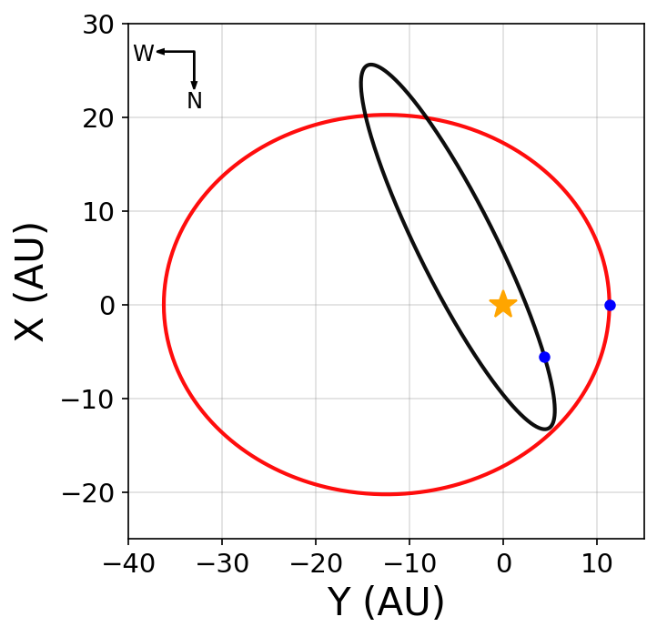
Fig. 1.6 Representation of the binary orbit with the orbital plane coplanar with the sky plane (red) and the observed orbit (black) using the appropriate Euler angles \((i,\ \omega, \&\ \Omega)\). The blue dots represent the pericenter of each orbit, where the black arrows denote the cardinal directions on the sky plane.#
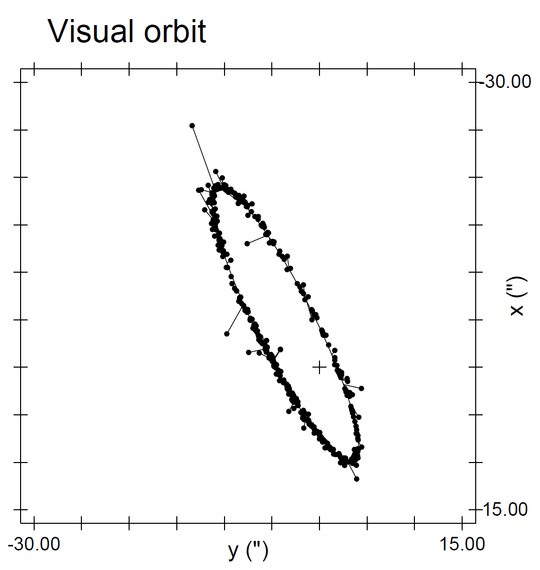
Fig. 1.7 Diagram illustrating visual orbit (on the sky) of \(\alpha\) Cen AB. Note that the units are given in arcseconds \((^{\prime\prime})\), where the distance to \(\alpha\) Cen AB \((1.334\ \rm pc)\) needs to used to convert arcseconds to AU. Figure credit: Pourbaix, Neuforge-Verheeke, & Noels (1999).#
Show code cell content
import numpy as np
import matplotlib.pyplot as plt
from matplotlib import rcParams
from myst_nb import glue

rcParams.update({'font.size': 14})
rcParams.update({'mathtext.fontset': 'cm'})

def Rotate_x(x,theta):
    R_x = np.array([[1,0,0],[0,np.cos(theta),-np.sin(theta)],[0,np.sin(theta),np.cos(theta)]])
    return np.dot(R_x,x)
def Rotate_y(x,theta):
    R_y = np.array([[np.cos(theta),0,np.sin(theta)],[0,1,0],[-np.sin(theta),0,np.cos(theta)]])
    return np.dot(R_y,x)
def Rotate_z(x,theta):
    R_z = np.array([[np.cos(theta),-np.sin(theta),0],[np.sin(theta),np.cos(theta),0],[0,0,1]])
    return np.dot(R_z,x)

def get_ellipse(rvec,omega,true_f,inc,RA):
    #get points of an ellipse given rvec (array), omega (constant), true anomaly f (array) and inclination (constant)
    ellipse = np.zeros((len(rvec),3))
    for i in range(0,len(rvec)):
        xp = Rotate_z(rvec[i,:],omega)
        xp = Rotate_x(xp,inc)
        ellipse[i,:] = Rotate_z(xp,RA)
    return ellipse

#Use the following for Alpha Cen AB:
semi = 23.78 # semimajor axis (in AU)
ecc = 0.524 #eccentricity
omg = np.radians(232.3) #argument of pericenter (converted to radians)
incl = np.radians(79.32) #inclination on the sky (converted to radians)
RA_omg = np.radians(204.75) #longitude of ascending node

fs = 'x-large'

f_step = 0.01
f = np.arange(0,2*np.pi+f_step,f_step)
r = semi*(1-ecc**2)/(1.+ecc*np.cos(f))
r_vec = np.zeros((len(r),3))
r_vec[:,0], r_vec[:,1] = r*np.cos(f), r*np.sin(f)

fig = plt.figure(figsize=(5,5),dpi=150)
ax = fig.add_subplot(111)

ax.grid(True,color='gray',alpha=0.25)
ax.set_aspect('equal')

ax.arrow(-33,27,-4,0,width=0.005,head_width=0.5,color='k',length_includes_head=True)
ax.text(-38.5,26,'W',horizontalalignment='center',rotation=0,fontsize='small')
ax.arrow(-33,27,0,-4,width=0.005,head_width=0.5,color='k',length_includes_head=True)
ax.text(-33,21,'N',horizontalalignment='center',rotation=0,fontsize='small')

ell = get_ellipse(r_vec,0,f,0,0)
#print(ell[0,:])
ax.plot(ell[:,0],-ell[:,1],'-',color='r',alpha=0.95,lw=2)
ax.plot(ell[0,0],-ell[0,1],'b.',ms=10)

ell = get_ellipse(r_vec,omg,f,incl,RA_omg)
ax.plot(ell[:,1],-ell[:,0],'-',color='k',alpha=0.95,lw=2)
ax.plot(ell[0,1],-ell[0,0],'b.',ms=10)
#print(ell[0,:])

ax.plot(0,0,'*',color='orange',ms=15)

ax.set_xlabel("Y (AU)",fontsize = fs)
ax.set_ylabel("X (AU)",fontsize = fs)
ax.set_xlim(-40,15)
ax.set_ylim(-25,30)

glue("alpha_Cen_AB", fig, display=False);
1.4. Coordinate systems#
The two body problem is defined in terms of six parameters that define the size and orientation of an ellipse relative to a central mass. In the case of a similar mass binary, the problem can be recast in either astrocentric or barycentric terms through a choice of a coordinate system. The definition of the ellipse is invariant to the choice of coordinate system (i.e., invariant through a Galilean transformation or translation). Mathematically, this means that we can transform from frame containing \(\{x,\ y,\ z\}\) to another frame with \(\{x^\prime,\ y^\prime,\ z^\prime\}\) by
where the coordinates \(\{x_o,\ y_o,\ z_o\}\) represent a point of reference. The velocities can be transformed in a similar way (e.g., \(v^\prime_x = v_x + v_{x,o}\)).
1.4.1. Barycentric coordinates#
Let’s define the center of mass as the point of reference with the vectors \(\vec{x_o} = \{x_o,\ y_o,\ z_o\}\) and \(\vec{v_o} = \{v_{x,o},\ v_{y,o},\ v_{z,o}\}\). Then an astrocentric frame can be constructed relative to the center of mass (or barycenter) for each of the masses using vectors \(\vec{x}_1\) and \(\vec{x}_2\) to locate the masses \(m_1\) and \(m_2\), respectively. A line can be constructed to connect one mass to the other through the barycenter, which introduces the following constraints:
which depends on the distance \(r = |\vec{x}_1-\vec{x}_2|\) between \(m_1\) and \(m_2\), the distance \(r_1 = |\vec{x}_1-\vec{x}_o|\) from the barycenter to \(m_1\), and the distance \(r_2 = |\vec{x}_2-\vec{x}_o|\) from the barycenter to \(m_2\). Through the constraint, \(r_1\) and \(r_2\) can be parameterized in terms of \(r\) and the masses by
The velocities can be transformed in a similar way, where
which depends on the relative speed \(v = |\vec{v}_1-\vec{v}_2|\) between \(m_1\) and \(m_2\), the speed \(v_1 = |\vec{v}_1-\vec{v}_o|\) relative to the barycenter, and the speed \(v_2 = |\vec{v}_2-\vec{v}_o|\) relative to the barycenter. Then the speeds of each body are defined by the mass ratios,
The above example demonstrates the conditions for a two-body problem, but this can be generalized to \(N\) bodies by locating the position and velocity vectors for the barycenter. Mathematically, these vectors are determined by a vector sum of the vectors locating each body, or
After locating the barycenter in both position and velocity, then the coordinates of each body can be translated (e.g., \(\vec{x}_1^\prime = \vec{x}_1-\vec{x}_o\)) so that the barycenter is a reference and coincides with the origin of the coordinate system. Figure 1.8 illustrates the barycentric orbit for \(\alpha\) Cen AB on the sky plane.
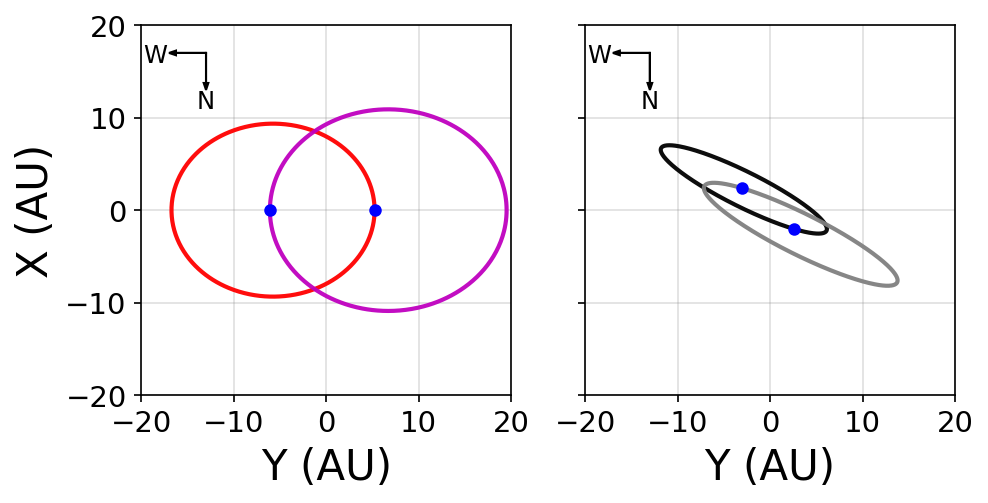
Fig. 1.8 Representation of the binary orbit (using barycentric coordinates) with the orbital plane coplanar with the sky plane (left) and the observed orbit (right) using the appropriate Euler angles \((i,\ \omega, \&\ \Omega)\).#
Show code cell content
import numpy as np
import matplotlib.pyplot as plt
from matplotlib import rcParams
from myst_nb import glue

rcParams.update({'font.size': 14})
rcParams.update({'mathtext.fontset': 'cm'})

def Rotate_x(x,theta):
    R_x = np.array([[1,0,0],[0,np.cos(theta),-np.sin(theta)],[0,np.sin(theta),np.cos(theta)]])
    return np.dot(R_x,x)
def Rotate_y(x,theta):
    R_y = np.array([[np.cos(theta),0,np.sin(theta)],[0,1,0],[-np.sin(theta),0,np.cos(theta)]])
    return np.dot(R_y,x)
def Rotate_z(x,theta):
    R_z = np.array([[np.cos(theta),-np.sin(theta),0],[np.sin(theta),np.cos(theta),0],[0,0,1]])
    return np.dot(R_z,x)

def get_rvec(a,e):
    r = a*(1-e**2)/(1.+e*np.cos(f))
    r_vec = np.zeros((len(r),3))
    r_vec[:,0], r_vec[:,1] = r*np.cos(f), r*np.sin(f)
    return r_vec

def get_ellipse(rvec,omega,true_f,inc,RA):
    #get points of an ellipse given rvec (array), omega (constant), true anomaly f (array) and inclination (constant)
    ellipse = np.zeros((len(rvec),3))
    for i in range(0,len(rvec)):
        xp = Rotate_z(rvec[i,:],omega)
        xp = Rotate_x(xp,inc)
        ellipse[i,:] = Rotate_z(xp,RA)
    return ellipse

def plot_ellipse(ax,r_vec,omega,true_f,inc,RA,col):
    ell = get_ellipse(r_vec,omega,true_f,inc,RA)
    ax.plot(ell[:,0],-ell[:,1],'-',color=col,alpha=0.95,lw=2)
    ax.plot(ell[0,0],-ell[0,1],'b.',ms=10)
    return

#Use the following for Alpha Cen AB:
semi = 23.78 # semimajor axis (in AU)
ecc = 0.524 #eccentricity
omg = np.radians(232.3) #argument of pericenter (converted to radians)
incl = np.radians(79.32) #inclination on the sky (converted to radians)
RA_omg = np.radians(204.75) #longitude of ascending node

m_1 = 1.133
m_2 = 0.972
m_tot = m_1 + m_2

fs = 'x-large'
f_step = 0.01
f = np.arange(0,2*np.pi+f_step,f_step)

r_vec1 = get_rvec(m_2/m_tot*semi,ecc)
r_vec2 = get_rvec(m_1/m_tot*semi,ecc)

fig = plt.figure(figsize=(7,5),dpi=150)
ax1 = fig.add_subplot(121)
ax2 = fig.add_subplot(122)
ax_list = [ax1,ax2]

for i in range(0,2):
    ax = ax_list[i]
    ax.grid(True,color='gray',alpha=0.25)
    ax.set_aspect('equal')
    ax.set_xlabel("Y (AU)",fontsize = fs)
    if i == 0:
        ax.set_ylabel("X (AU)",fontsize = fs)
    else:
        ax.set_yticklabels([])
    ax.set_xlim(-20,20)
    ax.set_ylim(-20,20)

    ax.arrow(-13,17,-4,0,width=0.005,head_width=0.5,color='k',length_includes_head=True)
    ax.text(-18.5,16,'W',horizontalalignment='center',rotation=0,fontsize='small')
    ax.arrow(-13,17,0,-4,width=0.005,head_width=0.5,color='k',length_includes_head=True)
    ax.text(-13,11,'N',horizontalalignment='center',rotation=0,fontsize='small')


plot_ellipse(ax1,r_vec1,0,f,0,0,'r')
plot_ellipse(ax1,r_vec2,np.pi,f,0,0,'m')

plot_ellipse(ax2,r_vec1,omg,f,incl,RA_omg,'k')
plot_ellipse(ax2,r_vec2,omg+np.pi,f,incl,RA_omg,'gray')

glue("alpha_Cen_AB_bary", fig, display=False);
1.4.2. Jacobi Coordinates#
Barycentric coordinates requires that all the bodies share a similar reference point (i.e., the barycenter). However, some systems are hierarchical (e.g., Sun-Earth-Moon) and it makes more sense to define the coordinate system following the hierarchy. For such systems, we use Jacobi coordinates that defines the next position and velocity relative to the barycenter of the inner subsystem.

Fig. 1.9 Diagram illustrating the Jacobi coordinates for a system of 4 bodies. The first two masses (\(m_1\) and \(m_2\)) have a barycenter that lies between them relative to the point \(O\). The third mass \(m_3\) is located relative to this barycenter by \(r_2\). The final mass \(m_4\) is located (by \(r_3\)) relative to the barycenter between \(m_3\) and the barycenter between \(m_1\) and \(m_2\). Each of the bodies are also located relative to the point \(O\) by \(x_1\), \(x_2\), \(x_3\), and \(x_4\), respectively. Image credit: Wikipedia:Jacobi_coordinates.#
Using Jacobi coordinates is an iterative process, where you need to keep track of the current position/velocity vector relative to a reference point \(O\) and the “inclusive” barycenter (or the barycenter of inner subsystem). For the \(j{\rm th}\) body \((1<j<N)\)
where the second term in the Jacobian \(\vec{x}_j^\prime\) and \(\vec{v}_j^\prime\) locates each inclusive barycenter. The \(N{\rm th}\) body will use the center of mass of the whole system and won’t require a translation.
Example
Using a system of 4 bodies, we have
\(\mathbf{j=1}\) |
\(\mathbf{j=2}\) |
\(\mathbf{j=3}\) |
\(\mathbf{j=4}\) |
|---|---|---|---|
\(\eta_1 = m_1\) |
\(\eta_2 = m_1 + m_2\) |
\(\eta_3 = m_1 + m_2 + m_3\) |
\(\eta_4 = m_1 + m_2 + m_3+m_4\) |
\(\vec{x}^\prime_1 = \vec{x}_1\) |
\(\vec{x}^\prime_2 = \vec{x}_2 - \vec{x}_1\) |
\(\vec{x}^\prime_3 = \vec{x}_3 - \frac{1}{\eta_2}\left[m_1\vec{x}_1 + m_2\vec{x}_2\right]\) |
\(\vec{x}^\prime_4 = \frac{1}{\eta_4}\left[m_1\vec{x}_1 + m_2\vec{x}_2 + m_3 \vec{x}_3 + m_4\vec{x}_4 \right]\) |
\(\vec{v}^\prime_1 = \vec{v}_1\) |
\(\vec{v}^\prime_2 = \vec{v}_2 - \vec{x}_1\) |
\(\vec{v}^\prime_3 = \vec{v}_3 - \frac{1}{\eta_2}\left[m_1\vec{v}_1 + m_2\vec{v}_2\right]\) |
\(\vec{v}^\prime_4 = \frac{1}{\eta_4}\left[m_1\vec{v}_1 + m_2\vec{v}_2 + m_3 \vec{v}_3 + m_4\vec{v}_4 \right]\) |
1.4.3. Converting orbital elements to Cartesian#
The orbital elements are defined relative to a central body problem (or a single central gravitational potential). However, a binary star system is not represented exactly by a central body, where there is now a binary potential. As a result, there are multiple ways of adding a third body to the binary system. One method is through a Galilean transformation, where the initial position \(\vec{x}_j\) and velocity \(\vec{v}_j\) of the stars and planets \((j= \{A,\ B,\ p\})\) are known using a Cartesian coordinate system.
Converting the binary orbit
The position vectors \(\vec{x}_A\) and \(\vec{x}_B\) represent the location of star A and B, respectively. Additionally these vectors can be determined using either an astrocentric or barycentric reference. Let’s assume an astrocentric reference (i.e., star A lies at the origin), where star B orbits star A and the binary orbital plane is coplanar with the reference plane \((i_B=\Omega_B=0^\circ)\). Therefore
directly represents the initial position and velocity of star A. We can use Eq. (1.1) and \(R_z(\omega_B + f_B)\) to get the position of star B within the orbital plane. Mathematically, this is
To find the velocity components from orbital elements, we can simply take the time derivative of the position vector before the rotation matrix \(R_z\) is applied to get
The \(\dot{r}\) can be determined through a time derivative of Eq. (1.1), while the \(r\dot{f}\) is determined using a form of Kepler’s 2nd law and the specific angular momentum (\(h = r^2\dot{f} = \sqrt{G(m_A+m_B)a(1-e^2)} = na^2\sqrt{1-e^2}\); see Eq. (1.9)) to get
Then we find
Finally, we can then apply the \(R_z\) rotation matrix to get
Adding the planet
To add the planet to initially orbit star A, we mostly follow the same procedure as for star B but replace with the planet’s orbital elements (e.g., \(r_p = a_p(1-e_p^2)/(1+e_p\cos{f_p})\)) that are defined relative to the host star.
The planetary inclination \(i_p\) and longitude of ascending node \(\Omega_p\) allow for the planet’s orbital planet to tilt relative to the binary orbital plane. To get a coordinates for the planet on the sky relative to the binary, we would simply apply the rotation matrices \(R_x\) and \(R_z\) as necessary using \(i_B\) and \(\Omega_B\).
In the case of the planet, it will have three Euler angles (\(i_p\), \(\omega_p\), \(\Omega_p\)) relative to the binary plane. As a result, we can apply the \(\left[R_z(\Omega_p)R_x(i_p)R_z(\omega_p)\right]\) matrix transformation onto a velocity vector that is similar to Eq. (1.32) to get
where \(n_p = \sqrt{G(m+m_p)/a_p^3}\) represents the mean motion of the planet relative to the host star with a mass \(m\). This will produce a set of Cartesian coordinates (\(\vec{x}_p\) and \(\vec{v}_p\)) such that
locate the planet’s initial coordinates relative to the host star. In this case, it is trivial to show that \(\vec{x}_p^\prime = \vec{x}_p\). For a planet orbiting star B, with star A as the reference it becomes non-trivial.
Note
This procedure is very general, but may not be the best/easiest way to setup the initial conditions. We are free to choose our reference, which means that we could have chosen star B as our reference instead so that the Galilean transformation wasn’t necessary. Moreover, we could have chosen the barycenter as our reference, which is most easily accomplished by first using an astrocentric reference first and then, transforming to the barycentric reference frame.