18. Relativity & Black Holes#
18.1. Time Dilation#
Hendrik Lorentz derived an expression that scales quantities by how fast they are moving relative to the speed of light. When this factor is applied to time, it stretches time in a process called time dilation. This factor (called the Lorentz factor) is abbreviated using \(\gamma\) and given by
Figure Fig. 18.1 shows how the value for the Lorentz factor changes with increasing speed \(v/c\), where Table Table 18.1 provides select numerical values of \(\gamma\) for a range of \(v/c\).
When moving at only \(0.5c\) (\(50\%\) of the speed of light), the Lorentz factor is \(1.15\), while something moving at \(0.9c\), it increases quickly to \(2.29\). Above \(0.9c\), the Lorentz factor increases exponentially large, but never reaches \(v/c = 1\).
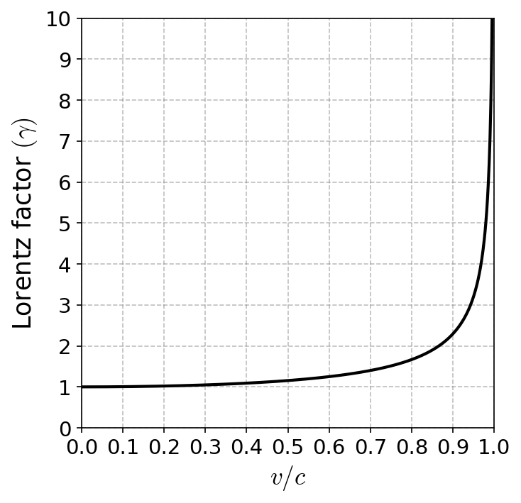
Fig. 18.1 The Lorentz factor \(\gamma\) as a function of \(v\c\). Note that it is not much different until \(v/c \sim 0.5\) and only reaches a factor of \(2\) at \(v/c \sim 0.9\).#
v/c |
\(\gamma\) |
|---|---|
0.10 |
1.005 |
0.20 |
1.02 |
0.30 |
1.05 |
0.40 |
1.09 |
0.50 |
1.15 |
0.60 |
1.25 |
0.70 |
1.40 |
0.80 |
1.67 |
0.90 |
2.29 |
0.95 |
3.20 |
0.99 |
7.09 |
0.995 |
10.01 |
0.999 |
22.37 |
Show code cell content
#Code to create Fig. 18.1
import numpy as np
import matplotlib.pyplot as plt
from matplotlib import rcParams
from myst_nb import glue

rcParams.update({'font.size': 14})
rcParams.update({'mathtext.fontset': 'cm'})

v_over_c = np.arange(0,1,0.001)
gamma = 1./np.sqrt(1-v_over_c**2)
fs = 'large'

fig = plt.figure(figsize=(5,5),dpi=150)
ax = fig.add_subplot(111)

ax.plot(v_over_c,gamma,'k-',lw=2)
ax.grid(True,alpha=0.5,color='gray',linestyle='--')

ax.set_xlabel("$v/c$",fontsize=fs)
ax.set_ylabel("Lorentz factor $(\gamma)$",fontsize=fs)
ax.set_xticks(np.arange(0,1.1,0.1))
ax.set_yticks(range(0,11))
ax.set_ylim(0,10)
ax.set_xlim(0,1)

glue("lorentz_fig", fig, display=False);
Suppose you take a trip to Proxima Centauri, which is \(4.25\ {\rm ly}\) away, to study the Earth-sized planet in orbit around it. You travel at \(0.2c\), whereas your twin stays behind on Earth. How long does your trip take for your twin back on Earth?
Your twin will measure the time using our common Newtonian experience, where
Note
Notice that we could effectively use \(c=1\) due to the definition of a light-year. If a light-year is the distance light travels in a year at a speed \(c\), then \((1\ {\rm ly})/c = 1\ {\rm year}\).
The round trip would take \(42.5\) years. When you return, you will find that \(42.5\) years have passed on Earth.
To you on the spaceship (moving at \(0.2c\)), time will pass more slowly. You will measure the time in the spaceship as
This is a relatively small difference, only \({\sim}1\ {\rm year}\). But for siblings, that’s a lot!
Suppose that your ship went a lot faster, say \(0.9c\). Your twin on Earth will measure
for the round trip time. You, on the other hand, will measure a round trip time of
Your twin will have aged \(9.44\) years, while you will have aged only \(4.12\) years.
import numpy as np
d_Prox_Cen = 4.25 #distance to Proxima Centauri in ly

def lorentz_factor(v_over_c):
    return 1./np.sqrt(1-v_over_c**2)

v_ship = 0.2 #speed of the spaceship relative to the speed of light
t_Earth = d_Prox_Cen/v_ship
t_ship = t_Earth/lorentz_factor(v_ship)
print("Assuming a ship that travels at 0.2c")
print("The trip time elasped on Earth for the twin is: %1.1f years." % (2*t_Earth))
print("The trip time you measure aboard the ship is: %1.1f years." % (2*t_ship))

print("----")
print("Adjusting the calculation for a faster ship at 0.9c")
v_ship = 0.9 #speed of the spaceship relative to the speed of light
t_Earth = d_Prox_Cen/v_ship
t_ship = t_Earth/lorentz_factor(v_ship)
print("The trip time elasped on Earth for the twin is: %1.2f years." % (2*t_Earth))
print("The trip time you measure aboard the ship is: %1.2f years." % (2*t_ship))
Assuming a ship that travels at 0.2c
The trip time elasped on Earth for the twin is: 42.5 years.
The trip time you measure aboard the ship is: 41.6 years.
----
Adjusting the calculation for a faster ship at 0.9c
The trip time elasped on Earth for the twin is: 9.44 years.
The trip time you measure aboard the ship is: 4.12 years.
For a more practical experiment, time dilation applies for subatomic particles. One type of particle (called a pion) exists for \(20\) nanoseconds (\(\rm ns\)) before it decays into different particles.
Suppose pions are produced in a particle accelerator moving at a speed of \(0.999c\), how long will physicists see the pions before they decay?
In the reference frame of the pions, they live for \(20\ {\rm ns}\). This is analogous to you in the previous example that was moving a high speed in a spaceship. Therefore, we know the pion’s trip time and are looking for how long the physicists perceive the trip time on Earth. With some algebra, we have
For an object moving at \(0.999c\), the value of \(\gamma = 22.37\). We can directly substitute to get
The physicists observe that pions moving at nearly the speed of light survive longer before they decay.
The Lorentz factor can also be applied to length. If a physicist measured the length of a ruler moving at \(0.999c\), the ruler would be \(22.37\times\) shorter than its length at rest.
18.2. Masses in X-ray Binaries#
Cygnus X-1 is a binary system with a blue supergiant (spectral type \(\rm O9.7\ I\)) and an unseen compact object located about \(0.2\ {\rm AU}\) away from it. The two objects orbit a common center of mass every \(5.6\ {\rm days}\). We can use the formula from 13.4 to calculate the sum of the masses,
where \(\rm BSG\) denotes the blue supergiant, \(a\) is the semimajor axis (in AU), and \(P\) is the orbital period of the binary (in years). We are almost ready to substitute our values, but we must first convert period to years (or \(P = 5.6/365.25 = 0.015\ {\rm yr}\)). We can then calculate the sum of the masses as
To find the values of the two individual masses, we need to know
the velocities of each object (i.e., like we did in 13.4 ), or
the distance of each object from the center of mass and the orbital inclination of the system.
It is difficult to obtain this information because one object is very compact and not observed separately. However the mass of the blue supergiant can be estimated from spectroscopic and photometric modeling (as long as the distance tot he system is known).
When that is done, the mass of the supergiant is \(19\ M_\odot\). Then we can find the mass of the compact object through subtraction to get \(15\ M_\odot\). This is well over the limit for a neutron star, therefore Cygnus X-1 is assumed to be a black hole. There are many ongoing studies to observationally determine the mass, where some of these are
which find that the compact object’s mass is \(10-22\ M_\odot\). The broader range of observational values shows that the observational estimates are model-dependent, which means there may be more than one accepted value.
a_bin = 0.2 #semimajor axis in AU
P_bin = 5.6/365.25 #orbital period converted from days to years

M_bin = a_bin**3/P_bin**2
print("The total mass of the binary is %1.2f solar masses." % M_bin)
The total mass of the binary is 34.03 solar masses.