19. Galaxies#
19.1. Finding the Distance from a Type Ia Supernova#
Type Ia supernovae can shine as bright as an entire galaxy at their maximum brightness, which makes them ideal to use as a standard candle. How do astronomers use Type Ia supernovae to estimate distance?
The first method uses the inverse-square law of light, which relates the flux \(F\) (or brightness), luminosity \(L\), and distance \(d\) by
We can do two things to the above formula: (1) rewrite it in terms of the solar constant \(F_\odot\ (=1361\ {\rm W/m^2})\) and (2) re-arrange it so that we solve for the distance \(d\) directly. We can get there by,
From the definition of parsec, we can use the following conversion factors:
or
Type Ia supernovae are typically measured in other galaxies (which are really far away), so let’s use the formula with \(\rm Mpc\):
From the above formula, we need to know the luminosity \(L\) of a Type Ia supernova and the observed flux \(F\) (in \(W/m^2\)). The typical maximum luminosity \(L\) of a Type Ia supernova is about \(9.5 \times 10^9\ L_\odot\).
In our textbook, it shows a picture of a Type Ia supernova in the Pinwheel Galaxy (M101). The maximum observed flux of the supernova was \(7.5\times 10^{-12}\ {\rm W/m^2}\). How far away is M101 in ly?
We can directly substitute the observed flux into our equation and find the distance to M101 in \(\rm Mpc\). Recall that \(1\ {\rm pc} = 3.26\ {\rm ly}\), which means that \(1\ {\rm Mpc} = 3.26 \times 10^6\ {\rm ly} = 3.26\ {\rm Mly}\).
First, finding the distance in \(\rm Mpc\) gives,
Now we must convert to \(\rm ly\) to get
Note that M101 is \(21\ {\rm Mly}\) away, which means that the supernova occurred about \(21\ {\rm million\ years}\) ago.
import numpy as np
L_max = 9.5e9 #maximum luminosity from a Type Ia supernova
F_SN = 7.5e-12 #observed flux from the supernova in M101
F_sun = 1361 #Solar constant (flux from the Sun at 1 AU)

d = (np.pi/6.48e11)*np.sqrt(L_max*F_sun/F_SN)
print("The Type Ia supernova places M101 %1.1f Mpc away." % d)
print("The Type Ia supernova places M101 %1.1e ly away." % (d*3.26e6))
The Type Ia supernova places M101 6.4 Mpc away.
The Type Ia supernova places M101 2.1e+07 ly away.
19.2. Calculating Recession Velocity and Galactic Distances#
We can determine a great deal using the equation for the Doppler effect (see Making use of the Doppler effect), where we measure the a spectral feature (in absorption or emission) is shifted in wavelength \(\lambda_{\rm obs}\) relative to the rest wavelength \(\lambda_{\rm rest}\). We have the Doppler effect equation for radial velocity \(v_r\) as
where \(c = 300,000\ {\rm km/s}\), or the speed of light. Recall that
\(\lambda_{\rm obs}-\lambda_{\rm rest} < 0\) corresponds to a blueshift because \(\lambda_{\rm obs}<\lambda_{\rm rest}\), and
\(\lambda_{\rm obs}-\lambda_{\rm rest}> 0\) corresponds to a redshift because \(\lambda_{\rm obs}>\lambda_{\rm rest}\).
For non-relativistic galaxy motion, we can replace the fraction in the Doppler equation with a single value \(z\). Note: there is a correction to \(z\) as you approach the speed of light. As a result, we now have
You’re observing nebulae in the 1920’s and taking measurements of using a spectrograph (see Fig. 19.1 below). You try to measure the \(H\ \alpha\) line at \(656.3\ {\rm nm}\) but find that it’s redshifted (see Table 19.1 below).

Fig. 19.1 Measurements of various nebulae from observations by Hubble (1929).#
NGC |
\(\lambda_{\rm obs}\) |
\(z\) |
\(v_r\) |
|---|---|---|---|
5457 |
656.738 |
0.0007 |
200 |
4736 |
656.934 |
0.0010 |
290 |
5194 |
656.891 |
0.0009 |
270 |
4449 |
656.738 |
0.0007 |
200 |
4214 |
656.956 |
0.0010 |
300 |
3031 |
656.366 |
0.0001 |
30 |
3627 |
657.722 |
0.0022 |
650 |
4826 |
656.628 |
0.0005 |
150 |
5236 |
657.394 |
0.0017 |
500 |
1068 |
658.313 |
0.0031 |
920 |
5055 |
657.284 |
0.0015 |
450 |
7331 |
657.394 |
0.0017 |
500 |
4258 |
657.394 |
0.0017 |
500 |
4151 |
658.400 |
0.0032 |
960 |
4382 |
657.394 |
0.0017 |
500 |
4472 |
658.160 |
0.0028 |
850 |
4486 |
658.050 |
0.0027 |
800 |
4649 |
658.685 |
0.0036 |
1090 |
Let’s use the data for NGC 5236, where \(\lambda_{\rm obs} = 657.394\ {\rm nm}\) and \(\lambda_{\rm rest} = 656.3\ {\rm nm}\). From those values, we can determine \(z\) by
Next, we can find the radial velocity by
which matches our table. Look’s like we’re doing it right.
Now, let’s find the distance to NGC 5236 using the Hubble constant \((H_o = 70\ {\rm km/s/Mpc})\). Hubble’s law is given by
where \(d\) is the distance in \(Mpc\). Using a little algebra, we find for NGC 5236
From the measurement of a spectral line, we can find that NGC 5236 is \(7.1\ {\rm Mpc}\) away. For comparision, Andromeda Galaxy (M31) is only \(0.77\ {\rm Mpc}\) away, which means that NGC 5236 is about \(10\times\) more distant than M31.
19.3. Size & Density of a SMBH#
19.3.1. Size of a SMBH#
The size of a black hole depends only on a single parameter, its mass. Recall the expression for the Schwarzschild radius \(R_s\), which relates the radius of the black hole (or event horizon) to the black hole mass \(M_{\rm BH}\), as
where \(G\) represents the contant of universal gravitation and \(c\) is the speed of light.
The largest supermassive black holes (SMBHs) observed have about \(10\ {\rm billion}\ M_\odot\). For example, the black hole at the center of M87 (a supergiant elliptical galaxy in Virgo) has a mass of \(6.69 \times 10^9 M_\odot\). We can easily find the size of this SMBH as
or \(20\ {\rm billion km}\). We can convert that value in to astronomical units (AU), where \(1\ {\rm AU} \approx 1.5\times 10^{8}\ {\rm km}\), by
The radius of the M87’s SMBH is large enough to engulf all of the Solar System planets (recall \(a_{\rm Nept} \approx 30\ {\rm AU}\)). It’s big enough to engulf a sizeable portion of the Kuiper belt too.
Note
We know that light takes \(8.3\ {\rm min}\) to travel \(1\ {\rm AU}\) (or the distance from the Earth to the Sun). This means that it would take light about \(1080\) light-minutes for light to traverse just the radius of M87, or around \(18\ {\rm hours}\) to travel from the event horizon to the center of the SBMH.
19.3.2. Density of a SMBH#
How compact (or dense) is the mass inside the event horizon? The mass of a SMBH can be measured by measuring the orbital period and semimajor axis of the star’s closest to them. The bulk (average) density of an object is determined by spreading all the mass uniformly into a sphere of radius \(R\). In this case, the radius of the sphere is the Schwarzschild radius \(R_s\), so that the density \(\rho_{\rm BH}\) is given by,
where we can make an approximation of the Schwarzschild radius \(R_s\) and make a substitution to get,
where \(R_\odot\) is a solar radius (\(6.957 \times 10^5\ {\rm km}\)) and \(\rho_\odot\) is the solar density \((1.41\ {\rm g/cm^3})\).
Consider the density of different SMBHs ranging from the Milky Way (\({\sim}4 \times 10^6\ {\rm M_\odot}\)) to M87. You want to express the density of the black hole \(\rho_{\rm BH}\) in normal units (i.e., \(\rm g/cm^3\)) and astronomical units \((\text{i.e., } M_\odot/{\rm AU}^3)\). Note that the mass of the M87’s SMBH is about \(1673\times\) the mass of the Milky Way’s SMBH.
Let’s find the density of the SMBH at the center of the Milky Way \(\rho_{\rm MW}\). Using our formula from above,
The SMBH of our own Milky Way is about \(781\times\) denser than the Sun.
Now let’s consider a more massive SMBH like the one at the center of M87. Since, we know about how much more massive the SMBH is compared to the Milky Way, we can use make use of our previous result by
That is about \(1/3\) the density of air at sea level \((\rho_{\rm air} = 1225\ {\rm kg/m^3})\) or about \(1/2500\) the density of water. Lower mass black holes are denser than SMBHs because the density scales with the inverse square of the mass, \(\rho_{\rm BH} \propto 1/M_{\rm BH}^2\).
Note
The conversion to astronomical units is straightfoward where you should find that \(1\ {\rm g/cm^3} = 1.68 \times 10^6\ M_\odot/{\rm AU}^3.\) In these units the solar density \(\rho_\odot = 2.36\ M_\odot/{\rm AU}^3.\) This seems like a lot, but remember that the Sun’s radius \(R_\odot = 0.00465\ {\rm AU}\) is really small.
Table 19.2 shows the estimated density of several different black holes (relative to the Milky Way’s SMBH), but it provides the density in astronomical units, cgs units, and relative to the solar density. Note that the values are correct to the nearest order of magnitude, where the uncertainty in the measurement of the SMBH mass is usually \(\gtrsim 5\%\).
SMBH Mass ($M_{\rm MW}) |
\(\rho_{\rm BH}\) \([M_\odot/\mathrm{AU}^3]\) |
\(\rho_{\rm BH}\) \([g/cm^3]\) |
\(\rho_{\rm BH}/\rho_\odot\) |
|---|---|---|---|
Milky Way (\(1\ M_{\rm MW}\)) |
\(1.8\times 10^9\) |
\(1100\) |
\(781\) |
Andromeda (\(35\ M_{\rm MW}\)) |
\(1.5\times 10^6\) |
\(0.89\) |
\(0.64\) |
M87 (\(1670\ M_{\rm MW}\)) |
640 |
\(3.9\times 10^{-4}\) |
\(2.79\times 10^{-4}\) |